Tephra4D: A Python-Based Model for High-Resolution Tephra Transport and Deposition Simulations—Applications at Sakurajima Volcano, Japan

Abstract

Vulcanian eruptions (short-lived explosions consisting of a rising thermal) occur daily in volcanoes around the world. Such small-scale eruptions represent a challenge in numerical modeling due to local-scale effects, such as the volcano’s topography impact on atmospheric circulation and near-vent plume dynamics, that need to be accounted for. In an effort to improve the applicability of Tephra2, a commonly-used advection-diffusion model, in the case of vulcanian eruptions, a number of key modifications were carried out: (i) the ability to solve the equations over bending plume, (ii) temporally-evolving three-dimensional meteorological fields, (iii) the replacement of the particle diameter distribution with observed particle terminal velocity distribution which provides a simple way to account for the settling velocity variation due to particle shape and density. We verified the advantage of our modified model (Tephra4D) in the tephra dispersion from vulcanian eruptions by comparing the calculations and disdrometer observations of tephra sedimentation from four eruptions at Sakurajima volcano, Japan. The simulations of the eruptions show that Tephra4D is useful for eruptions in which small-scale movement contributes significantly to ash transport mainly due to the consideration for orographic winds in advection.

1. Introduction

Volcanic eruptions release tephra to the atmosphere causing a hazard that can adversely affect the lives and livelihood of surrounding populations, leading to damages in sectors such as agriculture, forestry, fisheries. Furthermore, airborne tephra can be widely dispersed and have a serious impact on aircraft operations, as shown in the 2010 eruption of Eyjafjallajökull volcano [1]. For these hazard assessments, numerical simulations using advection-diffusion models are used to predict the dispersion of tephra in the atmosphere and the mass of tephra deposits [2].

After an eruption and the formation of a plume, tephra is advected by the wind, diffused due to turbulent processes, and descends due to its mass. In order to simulate the transport and deposition of tephra, numerical models require input parameters such as the plume height, total mass of tephra, wind field, and particle size, all of which are either based on observations, estimated, or simulated. Based on the meteorological conditions and the size of the eruptions, tephra transport and deposition can be simulated on scales of tens to hundreds of kilometers (e.g., [3,4,5]).

Tephra deposition prediction models that can reproduce small-scale eruptions are necessary for the study of volcanic plume dynamics. Up until now, most studies have focused on large-scale eruptions such as Plinian eruptions, but they have not been able to establish parameters such as the distribution of the segregation height of tephra in the plume (tephra segregation profile (TSP); e.g., [5,6]) and the interaction between particles and between particles and fluid (e.g., [7,8]). This is partly because large eruptions are infrequent, leading to the shortage of usable observations. Vulcanian eruptions present an opportunity to cover this lack of data due to their high frequency and relative safety of data acquisition.

For tephra transport numerical modeling to be suitable for vulcanian eruptions, it is first necessary to improve the consideration of the advection process. When tephra segregates from the plume at a low altitude from the surface of a volcano, it is important to take into account the bending of the ascending plume [9] and the heterogeneity of the wind field caused by the presence of the mountain (e.g., [10,11]).

When initializing a tephra transport simulation, it is common to assign grain size distribution to characterize the range of released particles. However, laboratory experiments have shown that the settling velocity of a particle of the same size depends on its effective density, shape, and whether or not it is bound to other particles (such as [6,12]), suggesting the importance of constraining the descent process not by the particle size distribution but by the settling velocity distribution. Due to the limitation of the observation, the particle size distribution has been assigned as the input parameter of the previous tephra deposit prediction model, and the settling velocity distribution was approximated from the particle size distribution based on the simple parameterizations. Particles with irregular effective density were calculated with an option (e.g., [13]) or neglected in these models. If the model handles a settling velocity distribution as an input parameter, such considerations can be made by simply changing the mass distribution without any special options.

In recent years, optical disdrometers have been increasingly used to observe tephra sedimentation [8,14,15] because they can measure the settling velocity of falling particles with a high temporal resolution. This allows for an alternative strategy: the characterization of the released tephra through a settling velocity distribution.

As such, in this study, we develop an advection-diffusion model Tephra4D based on the advection-diffusion model Tephra2 [3]. Tephra4D can take into account the spatial distribution of the time series of three-component wind velocity field and atmospheric density in the advection process and constrain the descent process by the settling velocity. Using disdrometer data from four eruptions from Sakurajima volcano, Japan, two sets of simulations are carried out. A simulation with the simple wind field is performed with a reimplemented model of Tephra2 constrained by the settling velocity distribution and simulations using the modified Tephra4D model. By comparing the results with the observations using a disdrometer network, we examine how the specification changes made in Tephra4D contribute to the improvement of the calculation and which points need further improvement.

The paper is structured as follows. Initially, the detailed calculation of the tephra deposit by Tephra4D is described in Section 2. Then the eruptions studied, model setup, and the results of the calculation are detailed in Section 3. In Section 4, we discuss the advantages of Tephra4D and important factors. Finally, Section 5 summarizes the main conclusions of the study.

2. Model Description

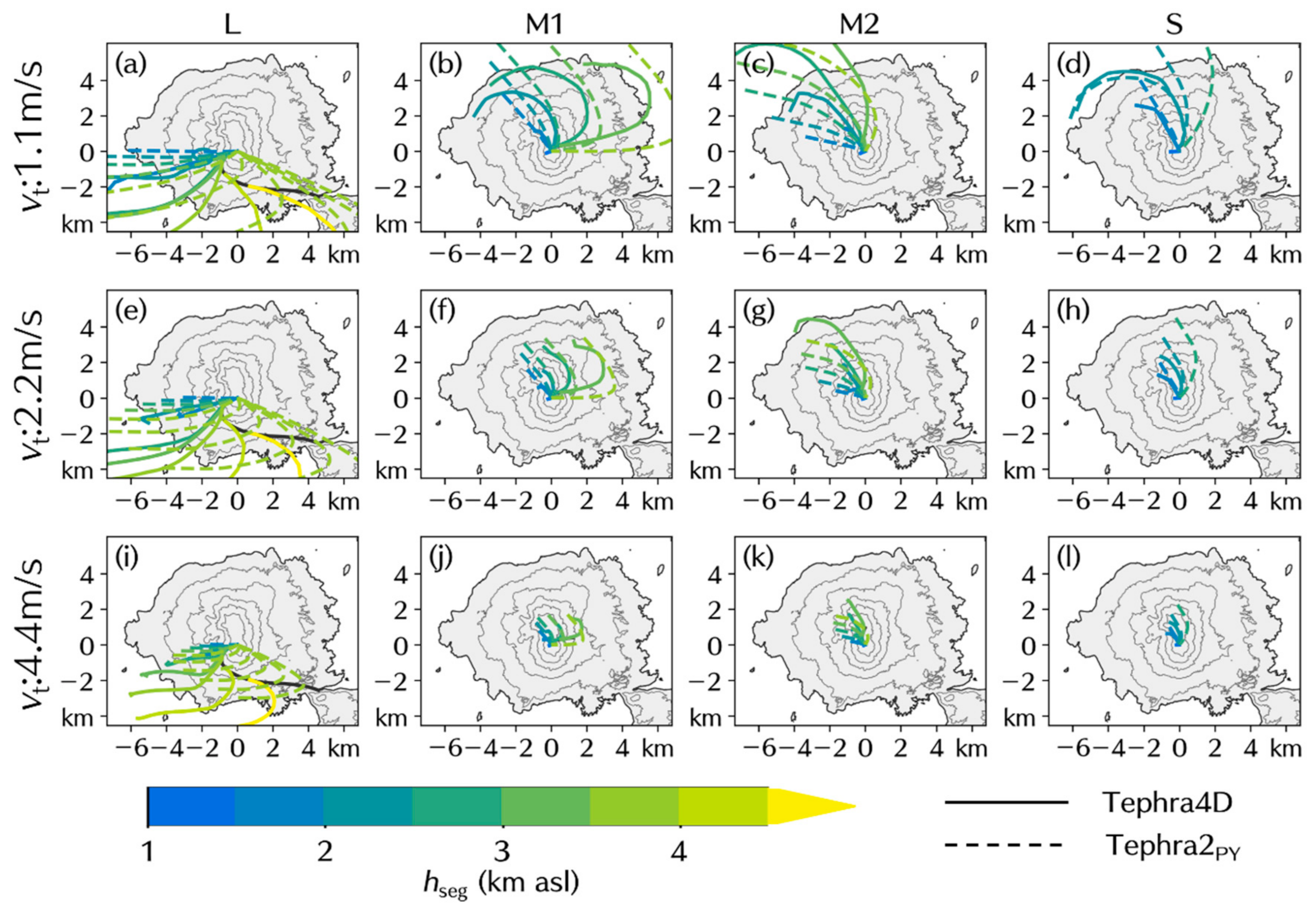
2.1. The Advection-Diffusion Model Tephra2 and Its Modifications

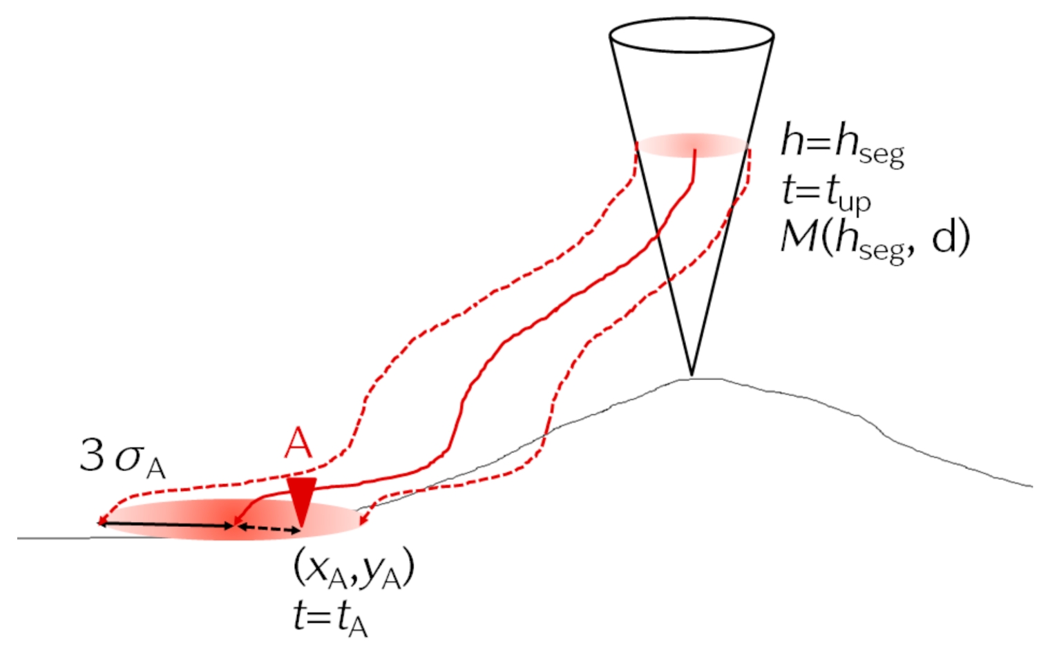
Tephra2 is an advection-diffusion model improved from the analytical model of [6], which numerically solves the equation of terminal velocity and dispersion [16]. The migration path of the center of gravity of the particle cluster as they segregate from the plume and fall into the atmosphere (hereinafter referred to as the “trajectory”) is calculated and then the tephra deposit load is obtained considering the diffusion process (Figure 1).

Tephra2 employs a horizontally homogeneous steady state, does not account for plume bending, and particles are classified by diameter. These aspects of the model need to be improved in order to successfully model vulcanian eruptions. We do this by employing temporally evolving wind fields obtained from the Weather and Research and Forecasting (WRF) model, including a mechanism for plume bending, and classifying the particles by terminal velocities instead of diameter. We refer to this improved model as Tephra4D.

A model that implements plume bending in Tephra2 was developed by [9], while in this study we implement another simple assumption. The vertical velocity when the plume rises is calculated in the same way as the particle falls. The ascending velocity and the horizontal coordinate of the segregation point are independent of the settling velocity.

Tephra4D takes into account wind heterogeneity in advection, but not in diffusion, and follows the assumption in Tephra2 that particles diffuse concentrically only in the horizontal direction. This is because the horizontal size of the plume is about 1.5 km, even for the largest plume in this study, and the horizontal wind is approximately uniform within this region. We reimplemented Tephra2 to use arbitrary TSP and settling velocity distributions as input parameters for control experiments. This reimplemented version is referred to as Tephra2_PY in this study. The difference of specifications among Tephra2, Tephra2_PY, Tephra4D are described in

Table 1. The specifications among three models.

Parameters	Tephra2	Tephra2PY	Tephra4D
Δhx (km)	-	-	≈0.3
Δt (min)	-	-	10
Continuity of σ at t = FTT	-	Equation (4)	Equation (4)
Plume bending	-	-	Equations (7) and (8)
vt distribution	Calculated from d	Directly substituted	Directly substituted
Wind below vent	Equation (10)	Equation (10)	Same as above vent (WRF)
ρa (h)	Equation (11)	Equation (11)	WRF
Settling velocity	[17]	[17]	Equation (15)
TSP	Equation (20)	Equations (17)–(20)	Equations (17)–(20)
Language	C	Python3	Python3

.

We prepare a representative particle corresponding to each settling velocity class. The movement of the center of gravity of a group of particles is calculated as the movement of the representative particle. The effective density of the particle is assumed to be 2640 kg/m³ [18]. The diameter and shape parameter of the particle are adjusted to take the same settling velocity as the median of the settling velocity class of the disdrometer at 0 m asl.

Let L_A (h_seg, d) be the areal concentration of particles of settling velocity v_t arriving at point A on the ground from a plume at the segregation height h_seg, then the tephra deposit load at point A S_A can be expressed as the sum of the areal concentrations of particles as a function of the segregation height and terminal velocity:

$$S_A={{\displaystyle \sum }}_{v_t}{{\displaystyle \sum }}_{h_{seg}}{\rho }_A\left(h_{seg},v_t\right)$$

(1)

Assuming that a falling particle cluster diffuses only horizontally and that the diffusion equation is expressed by a two-dimensional Gaussian distribution (variance σ) of the horizontal deviation (x, y) from the center of gravity of the particle cluster, the areal concentration L_A(h_seg, v_t) at point A, (x_A, y_A) away from the center when the center reaches an altitude of point A, is obtained from the following equation:

$$L_{\mathrm{A}}\left(h_{seg},v_t\right)=\frac{M\left(h_{seg},v_t\right)}{\pi {\sigma }_A{\left(h_{seg},v_t\right)}^2}\exp \left(-\frac{x_A^2+y_A^2}{{\sigma }_A{\left(h_{seg},v_t\right)}^2}\right)$$

(2)

where M is the mass of the particle cluster with settling velocity v_t segregated from the altitude h_seg and σ_A is the dispersion of the cluster at the altitude at which point A is located. Dispersion σ² is expressed as a function of dispersion time t and empirically given by an expression proportional to the first power of t when t does not exceed a threshold FTT (Fall Time Threshold) or an expression proportional to the 2.5 power of t when t exceeds FTT [6]. In this study, it is assumed that the horizontal spread of a plume is also caused by the diffusion of pyroclastic particles when the plume rises blowing in the wind. Assuming t = t_A (the time between the departure at the vent and the arrival at point A), σ² is calculated as follows:

$${\sigma }_A{\left(h_{seg},v_t\right)}^2=\left\{\begin{array}{r}4K{t}_A, | t_A<FTT\\ 1.6C{t}_A{}^{2.5}, | t_A\ge FTT\end{array}\right.$$

(3)

where K and C are the diffusion coefficient. FTT is defined to be 3600 s, the setting value in Tephra2, and considering the continuity of σ at t = FTT, which is not considered in Tephra2 and considered in Tephra2_PY, C is defined as follows:

$$C=\frac{2.5K}{FT{T}^{1.5}}$$

(4)

The relationship between the radius of the plume r and the elevation from the vent h is empirically given as follows [19]:

$$r=0.34h$$

(5)

and in Tephra2 and Tephra2_PY the following relationship is also given [3]:

$$r=3\sigma$$

(6)

This relationship is also followed in Tephra4D. Using Equations (3)–(6), the time between the departure at the vent and the segregation at altitude h_seg, t_up(h_seg), is obtained as follows:

$$t_{up}\left(h_{seg}\right)=\left\{\begin{array}{r}\frac{3.2\times {10}^{-3}{h}_{seg}^2}{K}, | t_{up}<FTT\\ {\left(\frac{8\times {10}^{-3}{h}_{seg}^2}{C}\right)}^{0.4}, | t_{up}\ge FTT\end{array}\right.$$

(7)

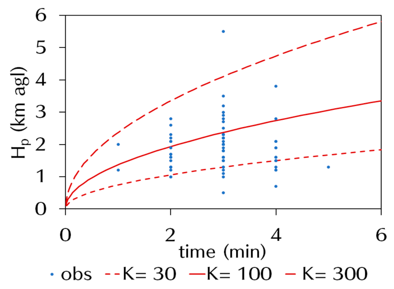
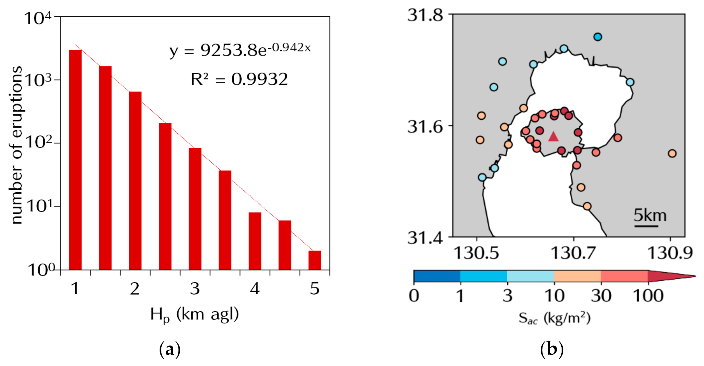
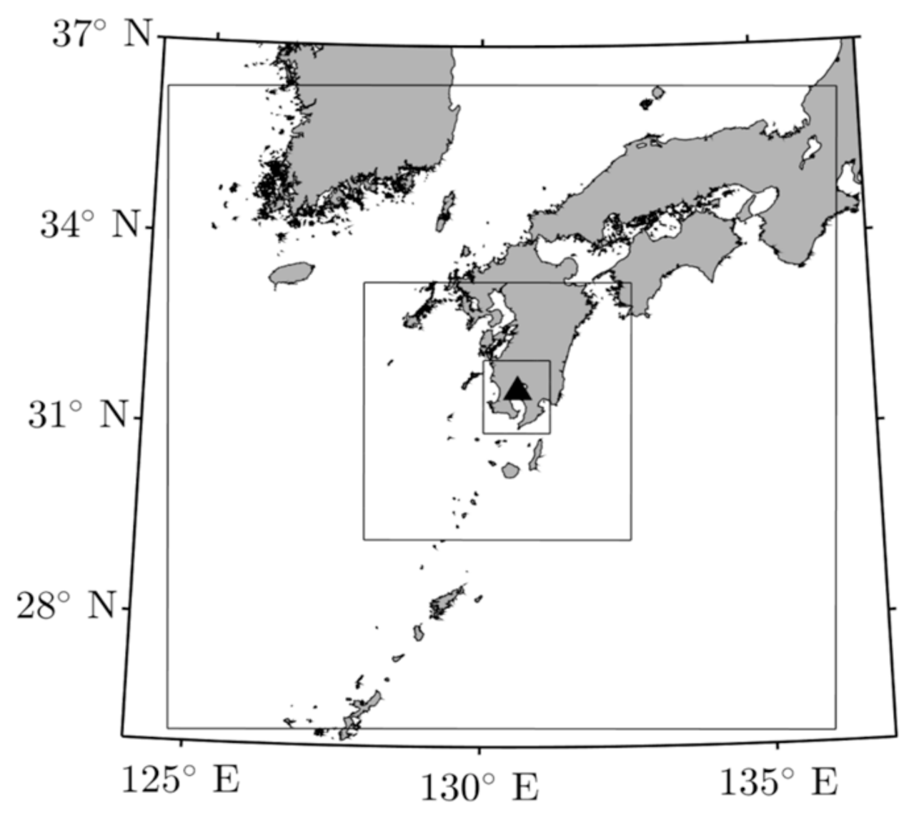
Applying Equations (3), (5) and (6) to a vulcanian eruption at Sakurajima, K was estimated from the time evolution of the plume top height. The height was read from the live camera image [20] every minute as shown in Figure 2. The optimal value is K = 100 m²/s although there is a large variation. The vertical velocity when particles rise through the plume is calculated based on Equation (7). We do not take into account the temporal variation of the mass eruption rate.

2.2. The Trajectory Calculation

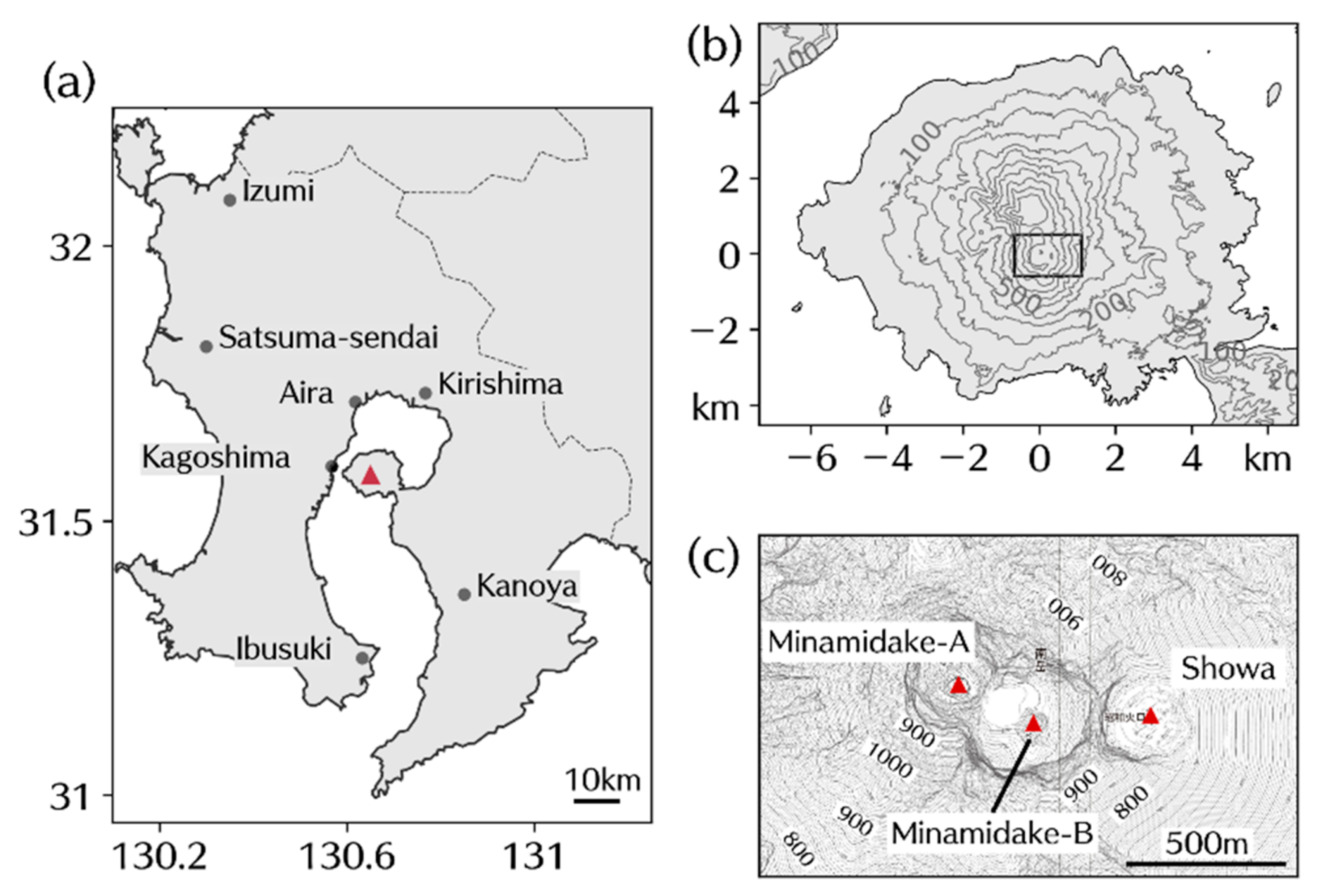
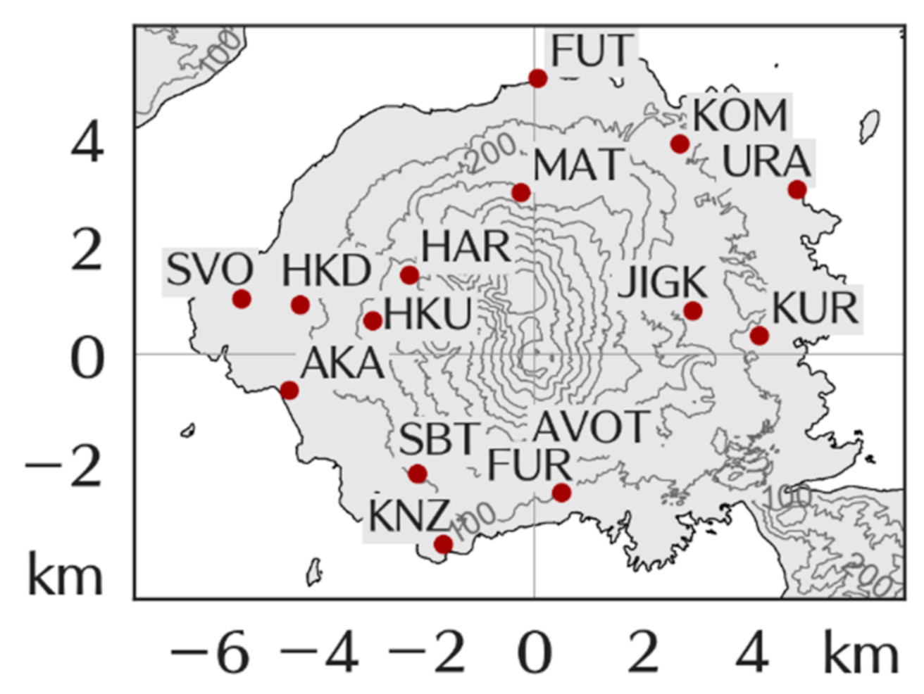
In the trajectory calculation, we consider a Cartesian coordinate system with the eastward, northward, and upward as the positive directions of x-, y-, and z-axis, respectively. Since the position of the meteorological field data is based on the UTM coordinate system in the horizontal direction and the altitude asl in the vertical direction, as shown in Figure 3, the particle exists in a hexahedron. The meteorological field inside this hexahedron is assumed to be a spatially homogeneous field represented by the value given to point C in

Table 2. The symbols to be used in trajectory calculation. The index n indicates nth step.

Symbol	Definition
z = z0, z1	The lower and the higher surface of the hexahedron.
A(x10, y10, z0), B(x11, y11, z0),C(x00, y00, z0), D(x01, y01, z0)	The coordinate of vertices of the lower surface.
(xn, yn, zn)	The coordinate of a particle inside a hexahedron.
(un, vn, wn)	The wind vector in the hexahedron.
vtn	The terminal velocity of the particle.
tn	Time to start.
Δtx, Δty, Δt𝑧	Time for the particle to reach the interface almost vertical to the x-, y-, and z-axis.

. The entire meteorological field will be composed of a large number of hexahedra, each with a homogeneous wind field and atmospheric density.

In each step, after the particle starts to move, the particle goes straight in the hexahedron, reaches the interface of the hexahedron, and moves to the next step in the neighboring hexahedron. The movement of the particle at nth step is expressed as the following recursion formula:

$$\left(\begin{array}{c}{x}_{n+1}\\ y_{n+1}\\ z_{n+1}\end{array}\right)=\left(\begin{array}{c}{x}_n\\ y_n\\ z_n\end{array}\right)+\min \left(\Delta t_x,\Delta t_y,\Delta t_z\right)\left(\begin{array}{c}{u}_n\\ v_n\\ w_n+v_{t,n}\end{array}\right)$$

(8)

Each symbol is described in Table 2. The recursion formula about time is as follows:

$$t_{n+1}=t_n+\min \left(\Delta t_x,\Delta t_y,\Delta t_z\right)$$

(9)

The same calculation is performed inside the hexahedron which the particle entered. If the particle moves to a neighboring hexahedron and then immediately returns to the original hexahedron, i.e., the hexahedron on which the particle resides at a given step is the same as the two steps earlier, the coordinate shift is calculated with the velocity component in the direction of boundary travel set to zero and the other velocity components set to the average of the velocity fields on the two hexahedra. Such a sequential calculation of trajectory is repeated until the particle reaches the ground or the horizontal limit of the calculation domain every indefinite spatial step. The calculation of Δt_x, Δt_y, Δt_𝑧 is detailed in Supplementary Material S1.

2.3. Wind Field and Atmospheric Density

Tephra4D uses temporally evolving three-component wind and atmospheric density data. The data were computed using the WRF model [21] with a horizontal grid spacing of 300 m, 58 layers in the vertical, and a temporal output of 10 min. The results from WRF are interpolated to a vertical grid to be used by Tephra4D. The detailed calculation of the wind field by WRF is described in Appendix C.

In Tephra2 and Tephra2_PY, the wind field is assumed to be horizontally uniform and does not have a vertical component. The wind field above the crater is interpolated from the wind speed and direction given by the user for each section. The wind speed at sea level is assumed to be zero and the wind speed v(h) at an altitude h asl under the crater is assumed as follows:

$$v\left(h\right)=\frac{h}{h_{vent}}v\left(h_{vent}\right)$$

(10)

where h_vent is the altitude of the vent asl. Assuming the density of fluid at 0 m asl as ρ_a0, the density of fluid ρ_a at the altitude h is calculated following the hypsometric formula:

$${\rho }_a\left(h\right)={\rho }_{\mathrm{a}0}\exp \left(-\frac{h}{8200}\right)$$

(11)

where the unit of h and 8200 is m.

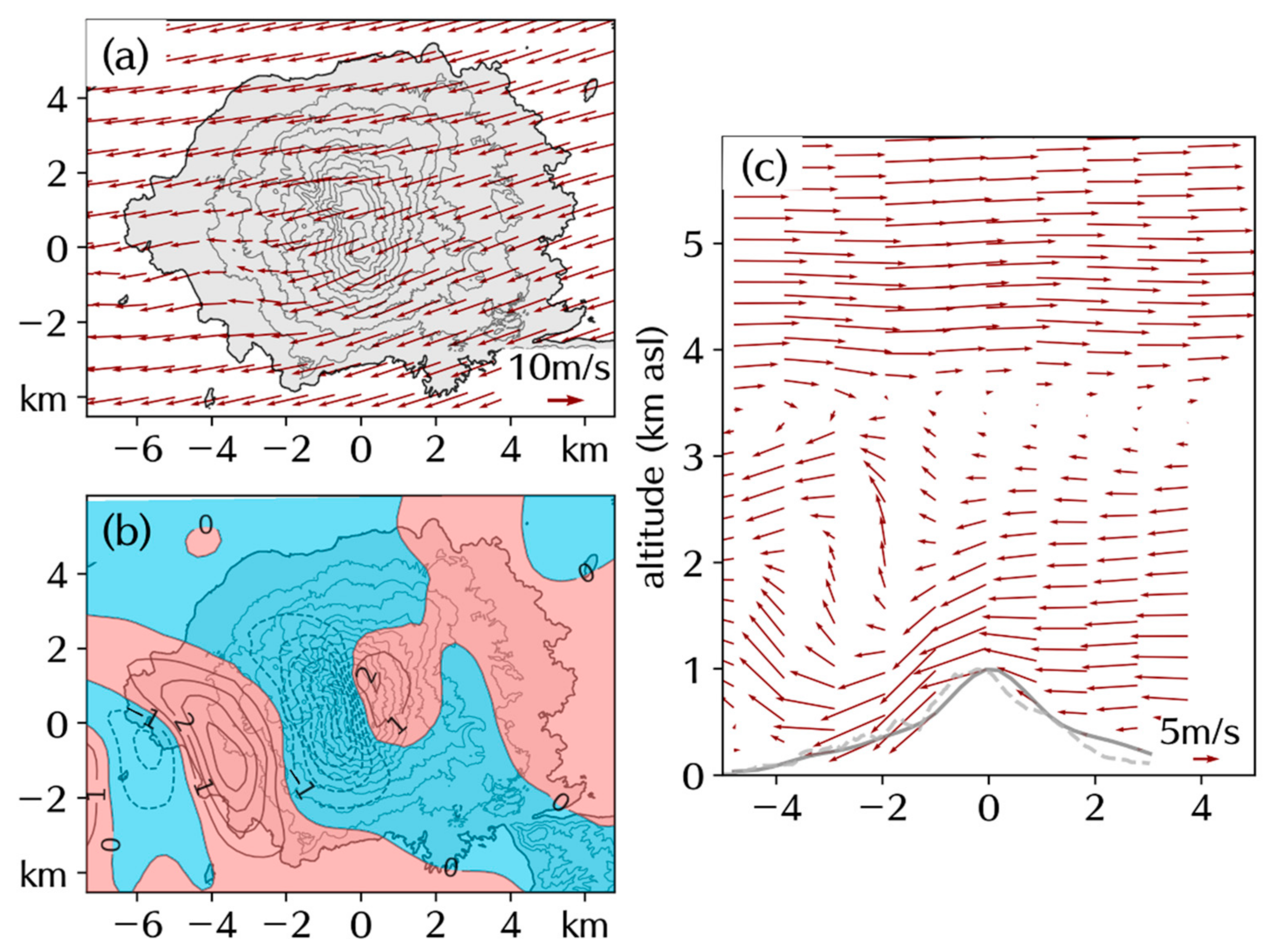
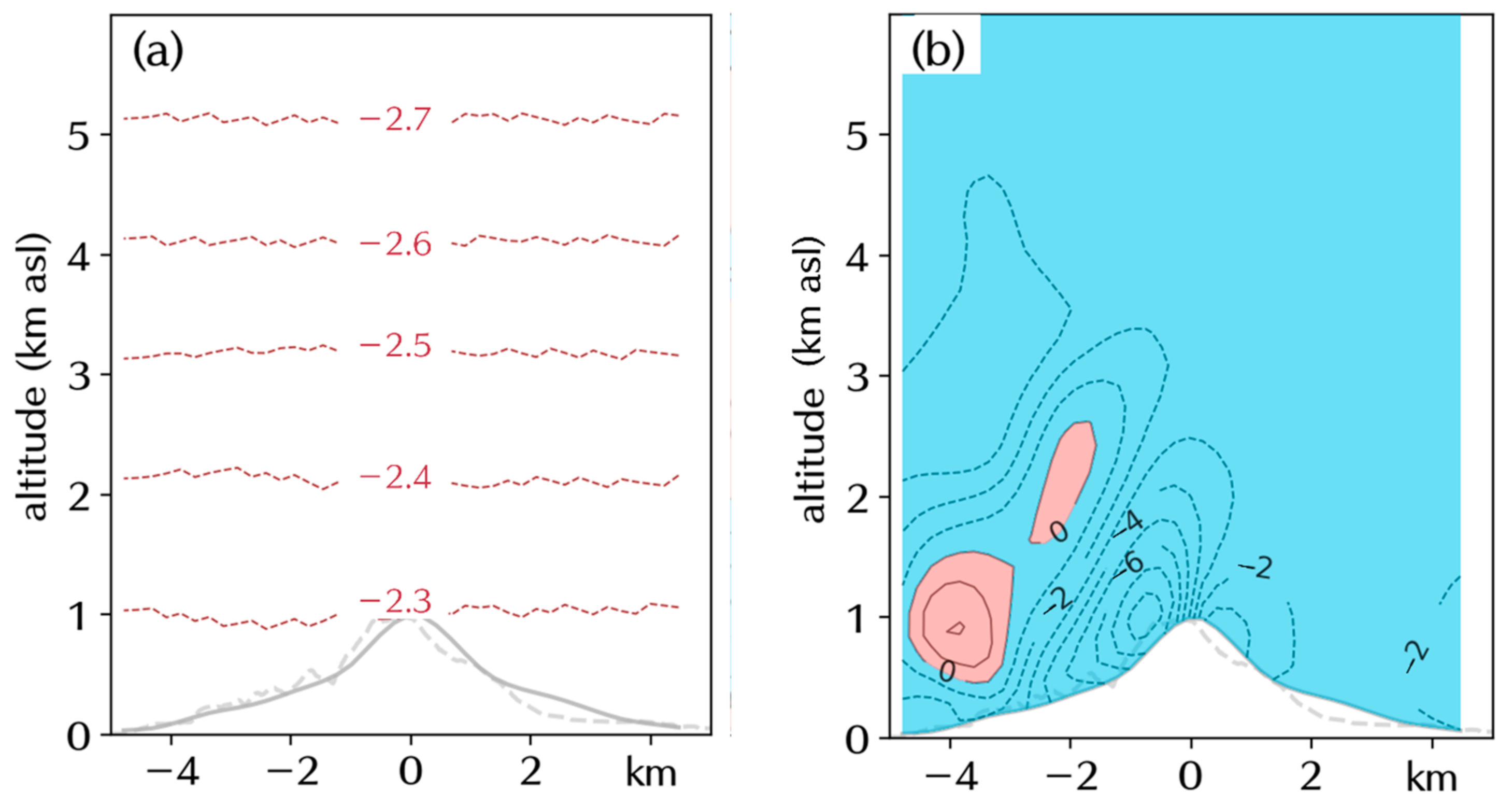
The simulated wind field for the eruption on 16 June 2018 is shown as an illustrative example. Tephra transport occurred to the west of the vent, agreeing with the resolved wind direction (Figure 4a). The atmospheric flow over the volcano is dominated by orographic waves, indicated by the oscillation seen in the west side (leeside) of the volcano (repeated pattern of downwards and upwards wind extending outwards) [22]. Such orographic activity has been shown to play an important role in the transport of tephra over complex topography [10].

2.4. The Settling Velocity of Pyroclastic Particles

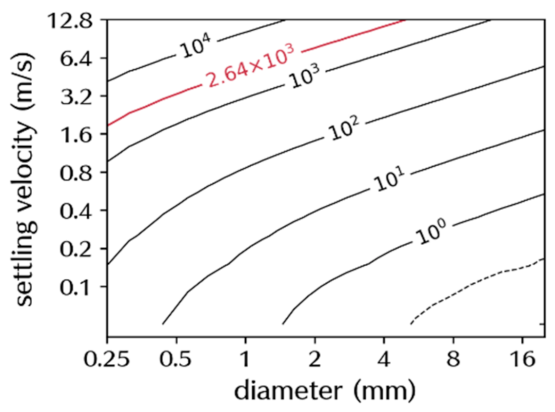
We consider that the difference in settling velocity for the same diameter corresponds to the difference in effective density due to the shape of the particles and the degree of agglomeration. We first obtain the relationship among the effective density of the pyroclastic particle ρ_p (kg/m³), the terminal velocity v_t (m/s), and particle diameter d (mm). Assuming that the shape of the pyroclastic particle is a spheroid, the relationship between ρ_p, v_t and d is represented by the following set of equations connected by the drag coefficient C_D and the Reynolds number R_a [6]:

$$v_t=\sqrt{\frac{4gd{\rho }_{\mathrm{p}}}{3C_D{\rho }_a}}$$

(12)

$$C_D=\frac{24}{R_a}{F}^{-0.32}+2\sqrt{1.07-F}$$

(13)

$$R_a=\frac{{\rho }_a{v}_{t}d}{{\eta }_{\mathrm{a}}}$$

(14)

where g is the gravitational acceleration, η_a, ρ_a are the viscosity and density of the surrounding fluid (i.e., the atmosphere in this study), and F is the shape parameter of the particles. Substituting Equations (13) and (14) into Equation (12) we get:

$$v_t=\frac{{\rho }_{\mathrm{d}}g{d}^2}{9{\eta }_{\mathrm{a}}{F}^{-0.32}+\sqrt{81{\eta }_{\mathrm{a}}^2{F}^{-0.64}+\frac{3}{2}{\rho }_{\mathrm{a}}{\rho }_{p}g{d}^3\sqrt{1.07-F}}}$$

(15)

Based on the diagram of the diameter and shape parameter F of the pyroclastic particles at Stromboli volcano [23], F is calculated using the following equation:

$$F=0.81+0.03{\log }_2\left(d/1000\right)$$

(16)

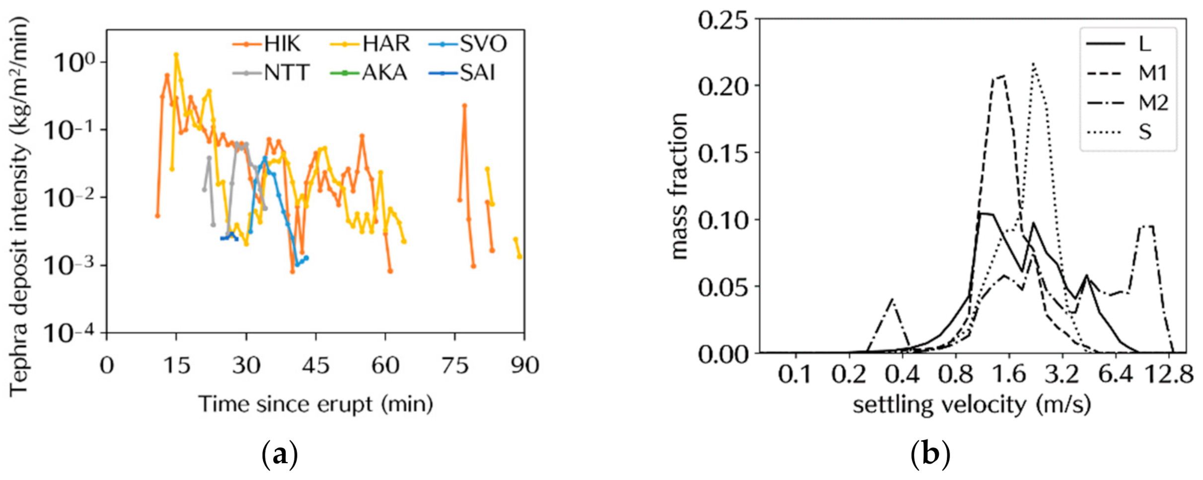
Assuming that v_t and d are equal to the settling velocity and particle size observed by the disdrometer, respectively, η_a, ρ_a are the values for the atmosphere at 20 °C, 1.8 × 10⁻⁵ Pa∙s, 1.205 kg/m³, the settling velocity, effective particle density is calculated as shown in Figure 5.

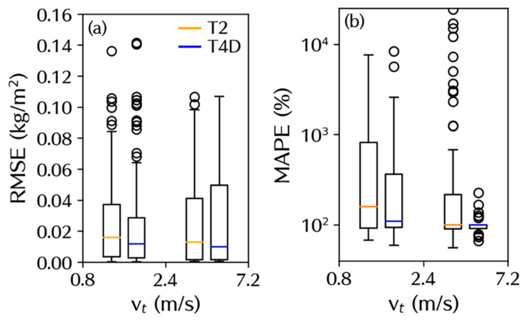
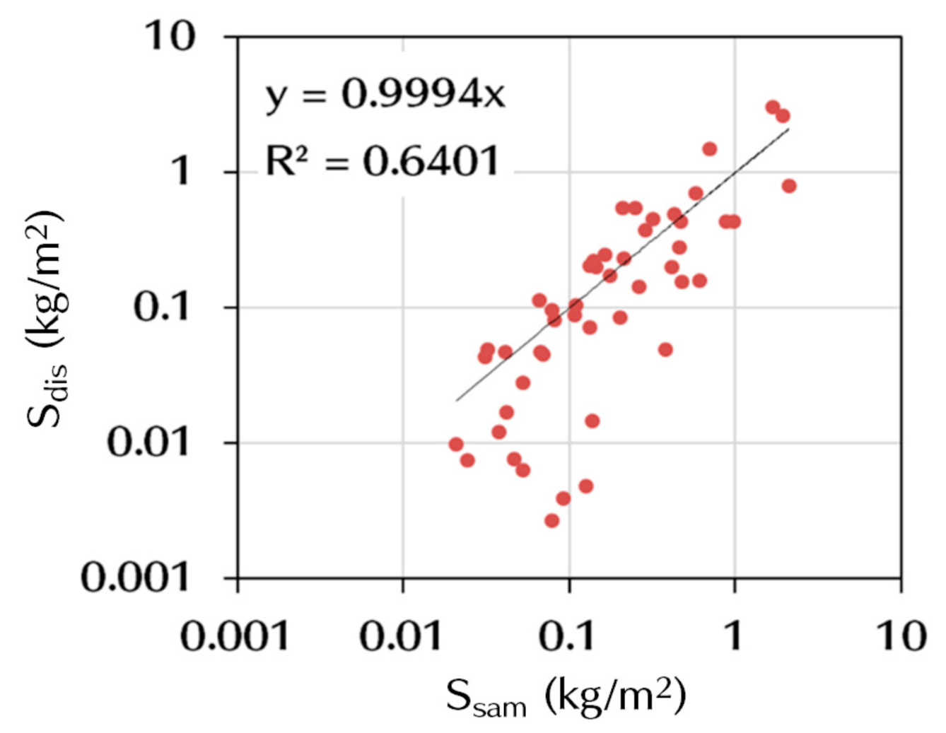
Tephra2 and Tephra2_PY calculates the terminal velocity from [17], while Tephra4D calculates it from Equation (15), which is used to calculate the observed tephra deposit load in Appendix B. As shown in Supplementary Material S2, the distance to reach the terminal velocity is negligible concerning the height of the plume top, so the particles are considered to have reached their terminal velocity when they are segregated from the plume. The spatial distribution of the terminal velocity of a pyroclastic particle with a terminal velocity of 2.2 m/s on the ground is shown in Figure 6a for the eruption on 16 June 2018. The terminal velocity decreased by about 20% between 5 and 0 km asl. Due to the influence of downward orographic wind to 3 km asl (Figure 6b), at the point where the downwind is strongest, the particle falls with 8.0 m/s in the settling velocity, which is the sum of the terminal velocity of 2.3 m/s plus the downward wind of 5.7 m/s. Thus, when strong mountain waves are formed, the change in settling velocity is more strongly affected by the change in the downward wind than by the change in atmospheric density.

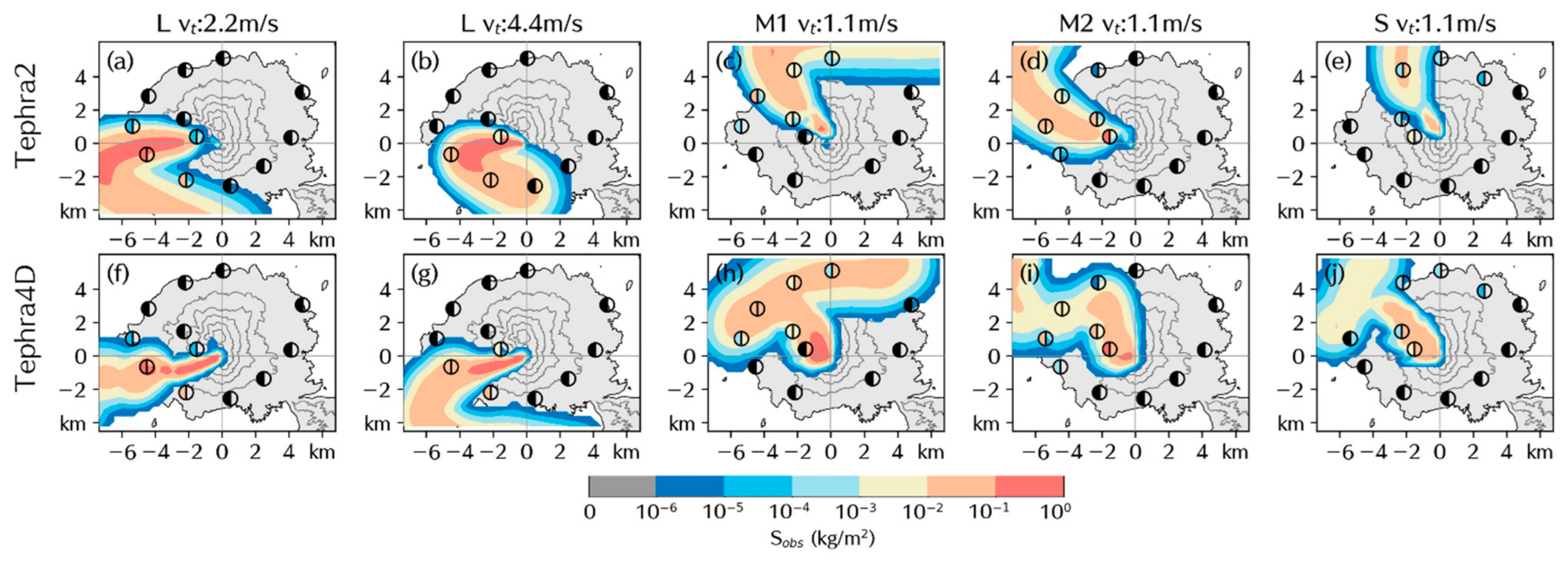
2.5. Tephra Segregation Profile

Since TSP M(h_seg, v_t), which is substituted in Equation (2), is highly arbitrary, it was constrained using the model of the distribution function. At an altitude interval of Δh, the mass of tephra with terminal velocity v_t at altitude h_seg discretized between the vent altitude h_vent to the plume altitude h_vent + h_plume is given by the following equation defining the function of TSP as m(h):

$$M\left(h_{seg},v_t\right)=M_{total}\left(v_t\right)\frac{{{\displaystyle \int }}_{h_{seg}}^{h_{seg}+\Delta h}m\left(h\right)dh}{{{\displaystyle \int }}_{-\infty }^{+\infty }m\left(h\right)dh}$$

(17)

where M_total(v_t) is the settling velocity distribution of the total mass fraction of tephra. In this study, the observed settling velocity distribution in each eruption is applied to M(v_t). We applied three distribution functions m(h) in this study.

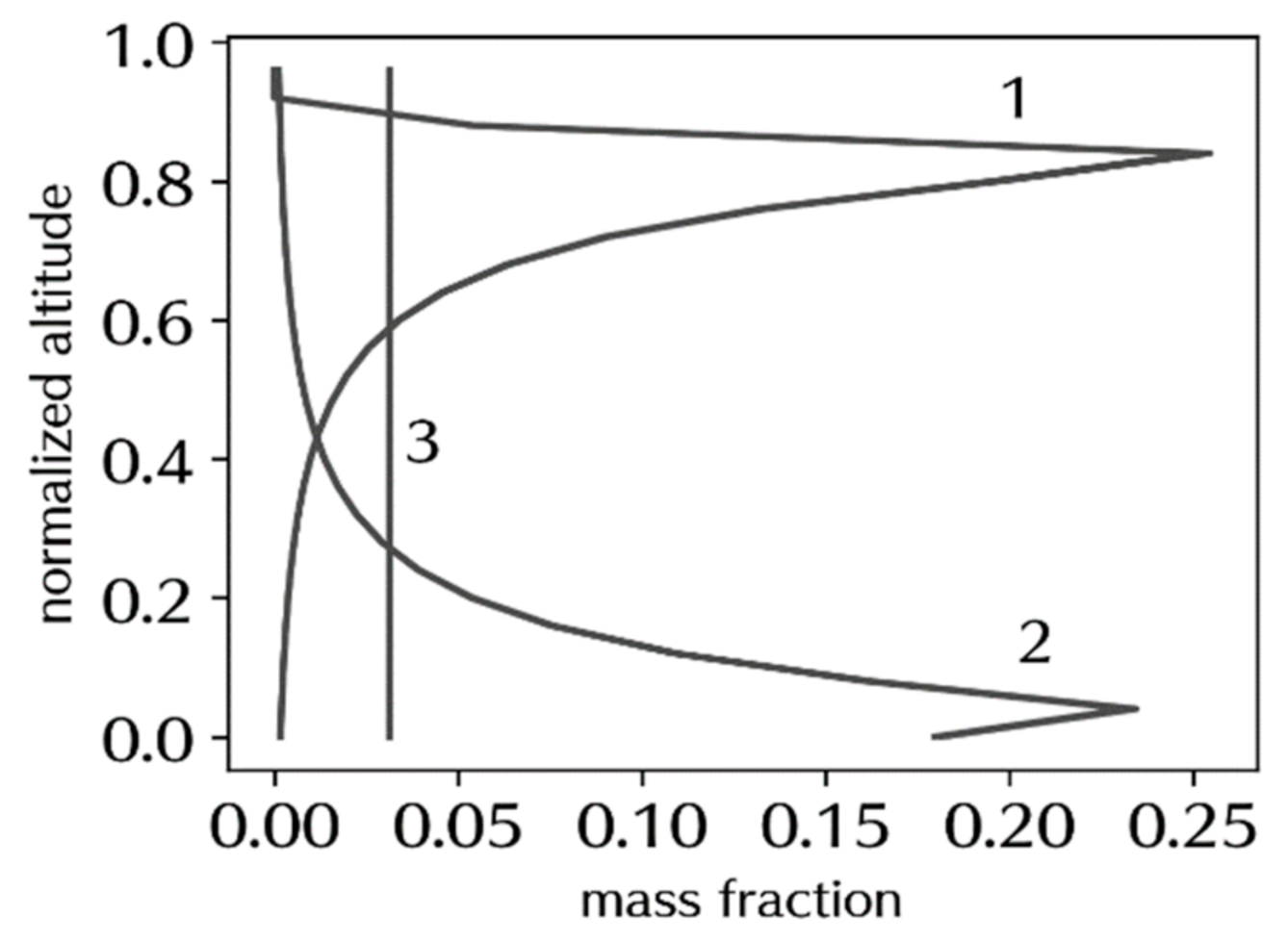
1. Logarithmic Gauss distribution with top concentration;

$$m\left(h\right)=\left\{\begin{array}{r}\frac{1}{\sqrt{2\pi }\left(h_{vent}+0.9 h_{plume}-h\right)}\exp \left(-\frac{1}{2}{\left(\log \frac{h_{vent}+0.9 h_{plume}-h}{0.1 h_{plume}}\right)}^2\right), | h<h_{vent}+0.9 h_{plume}\\ 0, | h\ge h_{vent}+0.9 h_{plume}\end{array}\right.$$

(18)

2. Logarithmic Gauss distribution with bottom concentration;

$$m\left(h\right)=\frac{1}{\sqrt{2\pi }\left(h-h_{vent}\right)}\exp \left(-\frac{1}{2}{\left(\log \frac{h-h_{vent}}{0.1 h_{plume}}\right)}^2\right)$$

(19)

3. Uniform distribution.

$$m\left(h\right)=\left\{\begin{array}{l}1, | h_{vent}+h_{plume}\ge h\ge h_{vent}\\ 0, | h>h_{vent}+h_{plume}\vee h_{vent}\ge h\end{array}\right.$$

(20)

These distributions are shown in Figure 7. TSP 1 and 2 have m(h) > 0 below the vent and above the plume top, respectively, and h_seg is restricted to the height from the vent to the plume top. As such, the sum of M in Equation (17) is smaller than M_total.

3. Benchmarking

3.1. The Eruptions Studied

In this study, we used eruptions from Sakurajima volcano, one of the most active and closely monitored volcanoes in Japan [24] to evaluate Tephra2_PY and Tephra4D. The eruptive activity of Sakurajima volcano is detailed in Appendix A. We analyzed four eruptions shown in

Table 3. Eruptions used as case studies.

id	Eruption Start	Plume Height (m agl)	Direction	Stations	Detected Sites	Ejecta (t)
L	2018/6/16 7:19	4700	W	12	4	22,000
M1	2018/5/29 3:34	2500	T	11	5	8100
M2	2018/6/9 21:27	2500	T	12	6	10,100
S	2018/11/27 9:01	1500	NE	12	5	3200

In the two eruptions where the direction of the flow was above the crater (T in the table), tephra deposit was detected at stations from north to west as seen from the crater.

that occurred at the Minamidake crater, one large eruption (L), two moderate eruptions (M1, M2), and one small eruption (S). A disdrometer network was installed on the island of Sakurajima to observe the tephra deposit load for error evaluation. The detailed observation is described in Appendix B. The height and direction of the plume tops are announced by JMA (eruptions L and M1), and in case the plume was obscured by clouds, they were estimated using the X-band MP radar image (eruptions M2 and S) [24,25]. Eruption volumes were calculated based on [26] from the strain changes associated with the eruption at Arimura (AVOT in Figure A4). The range of the plume height covers the typical height in Sakurajima (Figure A2a). The eruptions were chosen as they represent a range of typical eruptions from Sakurajima that led to tephra sedimentation over the volcano at a large number of disdrometers (≥4).

The temporal variation of the tephra deposit load at six sites associated with this eruption is shown in Figure 8a. Since vulcanian eruptions and subsequent continuous tephra emissions have different parameters such as plume height and TSP, we extract only the mass of pyroclastic particles ejected immediately after the eruption. To do this we consider that sedimentation from the initial explosion ends if there is a 10-min period of nondetection for each disdrometer location. For the analyzed sample, the settling velocity distributions of the tephra deposit load for the four eruptions were calculated according to Appendix B (Figure 8b) and applied to M_total(v_t) in Equation (17). The detected settling velocity range was widest and the heaviest tephra deposit was detected during eruption M2. The spatial distributions are shown in Figure 9. The azimuths of tephra deposit were distributed with the range of about 90° in all the eruptions. Eruptions L to S produced the largest tephra deposit in the west, northwest, west-northwest, and north, respectively. More than 1 kg/m² of tephra deposit was detected at a total of three sites in eruptions L and M2.

3.2. Model Setup

In this study, the settings in

Table 4. Model parameters applied in the simulations.

Parameters	Tephra2PY	Tephra4D
Δhz (km)	0.1	0.1
hvent (m asl)	1000	1000
ρa(0) (kg/m3)	1.205	1.205
K, C (m2/s, m2/s2.5)	100, 1.2 × 10−3	100, 1.2 × 10−3
FTT (s)	3600	3600
ηa (Pa s)	1.8 × 10−5	1.8 × 10−5

were applied. Δh is the vertical resolution of the wind field and the slice of plume model, h_vent is the altitude of the vent, Δt is the temporal resolution of the wind field, ρ_a(h) is the atmospheric density at the altitude h, K and C are the diffusion coefficients in Equation (3), and η_a is atmospheric viscosity.

3.3. Results Comparison

The trajectories of tephra calculated in Tephra2_PY and Tephra4D are shown in Figure 10. The horizontal position of the segregation point at the top of the plume was calculated almost the same as the horizontal coordinate of the vent in eruptions M1, M2, S, and in the same direction where the deposit was detected in eruption L. The maximum horizontal travel distance during ascent was calculated to be about 1.5 km, and the consideration of plume bending in this study does not seem to have a significant impact. Trajectories in Tephra4D change direction more frequently than those in Tephra2_PY, reflecting the consideration of horizontal heterogeneity in wind fields. The point reached on the ground is generally nearer in Tephra4D than in Tephra2_PY when particles segregate from low altitude and farther when particles segregate from high altitude. This is because the downward wind blows near the ground and the upward wind blows far from the ground in the region just leeward from the vent in the cases in this study (Figure 4c).

Based on these trajectories, the tephra deposit load distributions are calculated as shown in Figure 11. Overall the change in the way the wind field is used in the calculations can have a considerable impact. As with the trajectories, the most significant impact is seen close to the vent as enhanced deposition leads to larger deposit loads in the Tephra4D calculations.

We compared the calculation accuracy of Tephra2_PY and Tephra4D by the root mean square error (RMSE) and mean absolute percent error (MAPE) between calculated tephra deposit load S_cal and observed tephra deposit load by disdrometer S_obs. RMSE and MAPE are calculated using the following equations, respectively:

$$RMSE\left(er,v_t,TSP\right)=\sqrt{\frac{1}{N}{{\displaystyle \sum }}_{n=1}^N{\left(S_{cal}\left(er,v_t,TSP,n\right)-S_{obs}\left(er,v_t,TSP,n\right)\right)}^2}$$

(21)

$$MAPE\left(er,v_t,TSP\right)=\frac{1}{N}{{\displaystyle \sum }}_{n=1}^N\frac{S_{cal}\left(er,v_t,TSP,n\right)-S_{obs}\left(er,v_t,TSP,n\right)}{S_{obs}\left(er,v_t,TSP,n\right)}$$

(22)

where er, n are eruption and observation site, respectively. RMSE is shown in units of kg/m² while MAPE at a percentage. The sites where S_obs or S_cal is bigger than 0 are considered in Equation (21) and the sites where S_obs is bigger than 0 are considered in Equation (22). N is the number of considered sites. RMSE and MAPE are classified by the settling velocity class. The number of combinations of eruption, TSP, and settling velocity class where the number of sites where S_cal > 0 and S_obs > 0 N’, are shown in

Table 5. The number of combinations of eruption, TSP, and settling velocity class.

	0–0.8 m/s	0.8–2.4 m/s	2.4–7.2 m/s	7.2–22.4 m/s
N > 0	78	96	75	15
N’ > 0 (Tephra2PY)	16	96	59	12
N’ > 0 (Tephra4D)	58	96	43	3

. Based on the disdrometer observations, calculations using Tephra4D consistently improve results for particles with settling velocities less than 0.8 m/s but accuracy significantly drops for larger particles, particularly for settling velocities over 7.2 m/s.

The settling velocity groups where more than half of the combinations where N’ > 0 are 0.8–2.4 and 2.4–7.2 m/s. RMSE and MAPE distributions in these groups are shown in Figure 12. The ranges of RMSE are generally similar with a small but notable reduction in Tephra4D, while MAPE is reduced in Tephra4D especially with the settling velocity of 2.4–7.2 m/s. RMSE and MAPE distribution for the individual eruption is shown in Figure 13. Both RMSE and MAPE distributions improved significantly for the Tephra4D simulation in eruption L. In eruption M1, both the maximum and minimum of RMSE and MAPE reduced but the median increased with settling velocity 0.8–2.4 m/s. Accuracy was decreased based on both RMSE and MAPE and for both settling velocity groups in eruption M2. In eruption S, the maximum of RMSE and MAPE decreased but the minimum increased with settling velocity of 0.8–2.4 m/s.

4. Discussion

We estimated tephra deposits in four eruptions with various plume heights and wind fields in Tephra4D and Tephra2_PY. The tephra deposit load calculation is improved by Tephra4D in eruptions L and S compared with Tephra2_PY, were mostly unaffected in eruption M1, and worsened in eruption M2. The order of plume height is L, M1, M2, and S (M1 and M2 are the same), and there is no correlation between plume height and Tephra4D’s advantage. Since L was the eruption with the most dynamically moving trajectories during ascent and descent, and S was the eruption with the smallest plume height, Tephra4D is suggested to be useful for eruptions in which small-scale movement contributes significantly to ash transport.

The most significant reason for this advantage of Tephra4D is suggested to be the orographic wind consideration in the advection process, whose importance in tephra dispersion has been suggested in [10,27]. As shown in Figure 4b, strong downslope winds are present within 3 km of the crater, and the tephra deposit load near the crater was heavier in Tephra4D with vertical winds than in Tephra2_PY without vertical winds. Such difference in consideration into orographic winds affects the settling velocity range of tephra to deposit in the calculation. The settling velocity range where N’>0 is shown in

Table 6. The settling velocity range of the observed and estimated to be deposited at at least one observation site. Unit is m/s.

Observation/Model	L	M1	M2	S
Disdrometer	0.15–7.6	0.25–4.4	0.05–12	0.35–3.8
Tephra2PY	0.85–7.6	0.65–3	0.45–12	0.75–3
Tephra4D	0.35–7.6	0.45–2.6	0.15–4.4	0.35–2.6

. The lower limits of the velocity were more accurate in Tephra4D, while the upper limits of the settling velocity were more accurate in Tephra2_PY, suggesting that Tephra4D is useful for eruptions in which many particles with low settling velocity are ejected. The wind in the cases M1 and M2 was relatively weaker than that in the cases L and S leading to weaker orographic wave activity (Supplementary material S3). This can explain the lack of improvement for these two cases.

Despite the reproducibility of orographic winds in Tephra4D, Tephra2PY sometimes produces calculations more consistent with observations. This may be because Tephra4D does not take into account the orographic flows in the diffusion process. The movement of the particle cluster is represented by a single trajectory for each settling velocity and segregation height, and the diffusion of the particle cluster is considered to be concentric without considering the heterogeneity of the wind field. The wind heterogeneity in the cases L and S might be strong enough that the advantage of considering it in advection outweighed the disadvantage of not considering it in diffusion. Implementing the effect of orographic wind on diffusion, Tephra4D will contribute to the estimation of unknown parameters such as TSP and the interaction between particles and between particles and fluid.

The accuracy of the calculation of tephra dispersion affects the diffusion coefficient. When the diffusion coefficient is small, the accuracy of the calculation of the tephra deposit distribution is greatly affected by the accuracy of the particle movement estimation, and it is difficult to perform a highly accurate calculation in substituting a small diffusion coefficient. In this study, we applied 100 m²/s as K from the time evolution of the plume top height and the tangential width of tephra deposit are properly reproduced. In previous studies, K was estimated as shown in

Table 7. K applied in the previous studies.

Eruption	Plume Height (km)	K (m2/s)	Reference
Izu-Oshima, 1983	10–12	500	[5]
Ruapehu, 1996	8.5	1100	[28]
Etna, 2001	3.5–5	2000	[29]

and is longer than K in the present study. In the studies for the eruptions from Ruapehu [28] and Etna [29], diffusion during the plume rising was neglected and K on descent might be overestimated, but K in Tephra4D was small even taking it into account. Since these previous studies gave a horizontally homogeneous wind field, the diffusion coefficient likely compensated for the three-dimensional heterogeneity of the wind field. In Tephra4D, the heterogeneity in advection and the mountain wind contributed to the decrease in the diffusion coefficient compared to previous studies. By considering the heterogeneity in the diffusion as well as in the advection, we might calculate more accurate dispersion and reproduce the local variation of the tephra deposit load distribution more accurately.

5. Conclusions

The study of tephra dispersion from small-scale eruptions is required because of its high frequency. We created a new advection-diffusion model modified from Tephra2_PY in order to study small-scale eruptions, which need to consider local deviations of wind fields. Two advection-diffusion models with different wind fields and ascending plume trajectories were used to calculate the tephra deposit load distribution for the vulcanian eruptions from Sakurajima volcano, Japan.

Results from Tephra4D, the model developed in this study, show a shift in the deposition of tephra closer to the vent compared to the conventional model and enhanced lateral diffusion of the tephra cloud leading to wider deposition patterns. The model is expected to be useful for eruptions in which small-scale movement contributes significantly to ash transport. The main factor that led to these differences was the consideration of orographic winds. The comparison against results using Tephra2_PY shows reduced errors by considering the heterogeneity of the wind field, potentially leading to improvement in our study to establish unknown parameters in plume dynamics.