Article

The Diurnal Variation in Stratospheric Ozone from MACC Reanalysis, ERA-Interim, WACCM, and Earth Observation Data: Characteristics and Intercomparison

1
Institute of Applied Physics, University of Bern, 3012 Bern, Switzerland
2
Oeschger Center for Climate Change Research, University of Bern, 3012 Bern, Switzerland
3
Belgium Institute of Space Aeronomy, 1180 Brussels, Belgium
4
ECMWF, Shinfield Park, Reading RG2 9AX, UK
5
Institute of Environmental Physics, University of Bremen, 28359 Bremen, Germany
6
BC Scientific Consulting LLC (USA), Dunedin 9010, New Zealand
7
Department of Astronomy, University of Massachusetts, Amherst, MA 01003-9305, USA
8
Department of Environmental Chemistry and Engineering, Tokyo Institute of Technology, Tokyo 152-8550, Japan
9
Terahertz Technology Research Center, National Institute of Information and Communications Technology, Tokyo 184-8795, Japan
*
Author to whom correspondence should be addressed.
Current address: AWK Group AG, 3008 Bern, Switzerland.
Submission received: 7 April 2021 / Revised: 6 May 2021 / Accepted: 10 May 2021 / Published: 13 May 2021
(This article belongs to the Section Air Quality)

Abstract

:
In this study, we compare the diurnal variation in stratospheric ozone of the MACC (Monitoring Atmospheric Composition and Climate) reanalysis, ECMWF Reanalysis Interim (ERA-Interim), and the free-running WACCM (Whole Atmosphere Community Climate Model). The diurnal variation of stratospheric ozone results from photochemical and dynamical processes depending on altitude, latitude, and season. MACC reanalysis and WACCM use similar chemistry modules and calculate a similar diurnal cycle in ozone when it is caused by a photochemical variation. The results of the two model systems are confirmed by observations of the Superconducting Submillimeter-Wave Limb-Emission Sounder (SMILES) experiment and three selected sites of the Network for Detection of Atmospheric Composition Change (NDACC) at Mauna Loa, Hawaii (tropics), Bern, Switzerland (midlatitudes), and Ny-Ålesund, Svalbard (high latitudes). On the other hand, the ozone product of ERA-Interim shows considerably less diurnal variation due to photochemical variations. The global maxima of diurnal variation occur at high latitudes in summer, e.g., near the Arctic NDACC site at Ny-Ålesund, Svalbard. The local OZORAM radiometer observes this effect in good agreement with MACC reanalysis and WACCM. The sensed diurnal variation at Ny-Ålesund is up to 8% (0.4 ppmv) due to photochemical variations in summer and negligible during the dynamically dominated winter. However, when dynamics play a major role for the diurnal ozone variation as in the lower stratosphere (100–20 hPa), the reanalysis models ERA-Interim and MACC which assimilate data from radiosondes and satellites outperform the free-running WACCM. Such a domain is the Antarctic polar winter where a surprising novel feature of diurnal variation is indicated by MACC reanalysis and ERA-Interim at the edge of the polar vortex. This effect accounts for up to 8% (0.4 ppmv) in both model systems. In summary, MACC reanalysis provides a global description of the diurnal variation of stratospheric ozone caused by dynamics and photochemical variations. This is of high interest for ozone trend analysis and other research which is based on merged satellite data or measurements at different local time.

Foreword

The present study is the thorough revision of Schanz et al. (2014) [1] which was a preliminary study published in Atmospheric Chemistry Physics Discussion. The key figures (Figures 5 and 9) of the present study are improved and quite different from those of Reference [1]. The differences are mainly due to shortcomings in the derivation of the diurnal ozone amplitude in Reference [1]. While Figure 9 of Reference [1] shows zonal asymmetry of the diurnal ozone amplitude, the present study shows a zonally symmetric diurnal amplitude of polar stratospheric ozone. This finding of zonal symmetry supports the study of Frith et al. (2020) [2], who derived a model-based climatology of the diurnal amplitude of stratospheric ozone as function of latitude. The present study is an improved documentation of our past efforts in 2015 which corrects the errors in Reference [1]. We hope that the present study inspires new investigations about the diurnal ozone cycle in the middle atmosphere based on new observations and reanalysis datasets from ERA5 [3], MERRA-2 [4], SD-WACCM [5], CAMS (formerly MACC) [6], and others.

1. Introduction

Biases in satellite-based ozone trend analysis due to measurements at different local time and drifting satellite orbits renewed the interest in diurnal variations of stratospheric ozone [7]. Model projections indicate a recovery of the ozone layer of about 1% per decade [8,9,10,11,12] while the diurnal variation in stratospheric ozone typically has an amplitude of 2–4%. Such a strong diurnal ozone variation has to be adequately considered in the ozone trend analysis of satellite observations, particularly, when the satellite orbit slowly drifts in local solar time at a certain geographical location over a time scale of years [13].
The diurnal variation in stratospheric ozone was investigated by new studies based on chemistry–climate model simulations, ground-based microwave radiometry, and satellite observations, e.g., References [14,15,16]. Ref. [17] investigated the global, seasonal and regional behavior of diurnal variation in stratospheric ozone by means of the free-running Whole Atmosphere Community Climate Model (WACCM). The study explained the basic underlying physical processes as temperature-dependent photochemical reactions within the Chapman cycle and the catalytic odd nitrogen ( NO x ) cycle, which are the main contributors to the diurnal variation in stratospheric ozone. This photochemical variation during daytime in the stratosphere has a seasonality especially at high latitudes. The maximum ozone variation during a day is up to 0.8 ppmv (15%) at the polar circles in summer according to simulations of WACCM [17]. This surprisingly strong amplitude seemed to agree with measurements by a ground-based microwave radiometer at Ny-Ålesund, Svalbard [18]. Such strong diurnal variations would indicate that a correction of diurnal sampling effects in stratospheric ozone data sets is more needed than previously expected.
Ref. [14] compared the diurnal variation in stratospheric ozone from nudged chemistry–climate model simulations (SD-WACCM where SD stands for specified dynamics) to observations from the Superconducting Submillimeter-Wave Limb-Emission Sounder (SMILES) [19]. The SMILES observations showed a good agreement in the tropics to SD-WACCM [14], which nudges dynamics in the atmosphere up to 50 km. The wind and temperature fields of the model are nudged at every time step toward the meteorological reanalysis (Goddard Earth Observing System 5 (GEOS5) analysis) by 10%.
Ref. [15] derived the diurnal variation in stratospheric ozone using 18 years of microwave radiometer measurements at Mauna Loa (Hawaii). They compared the observed results to simulations of the Goddard Earth Observing System Chemistry Climate Model (GEOSCCM) [20,21,22] with two different implementations of atmospheric chemical processes. The observed and the simulated diurnal variation in stratospheric ozone agreed mostly within 1% (2 σ ) of the estimated statistical errors. Reference [23] derived a climatology of the diurnal ozone variation using a 17 years series of stratospheric ozone profiles measured by a microwave radiometer at Bern, Switzerland. They found indications for an inter-annual variability of the diurnal ozone variation.
The good agreement of model data and observations may indicate that a model-assisted correction of diurnal sampling effects in satellite ozone measurements could be feasible. Alternatively to a model-assisted correction of satellite data, the assimilation of satellite ozone measurements into an advanced chemistry–climate model with two-way interactions between dynamics and atmospheric composition may be considered. The European Union’s Earth observation program Copernicus develops such a chemistry–climate model system called Monitoring Atmospheric Composition and Climate (MACC). MACC assimilates satellite data of atmospheric composition, including ozone, into a global atmosphere model to provide a reanalysis of atmospheric composition for the years 2003–2012. Such a model system might help to correct diurnally sampled ozone data from biased satellite measurements and finally improve the quality of ozone trend estimates.
The present study follows on Reference [17] and compares the WACCM results to reanalysis data of the MACC project and the European Center for Medium-Range Weather Forecast’s (ECMWF) ERA-Interim. The diurnal ozone variation from MACC reanalysis, ERA-Interim and WACCM is confirmed by selected ground-based observations of the Network for the Detection of Atmospheric Composition Change ([24], NDACC, https://www.ndacc.org, accessed on 12 May 2021) and satellite-based observations of the Superconducting Submillimeter-Wave Limb-Emission Sounder (SMILES). Such intercomparison is of great interest for the correction of satellite data. In the Arctic region the OZOne Radiometer for Atmospheric Measurements (OZORAM) reveals the strong diurnal variation near the polar circle which has previously been simulated only. These results are intercompared to the data of the model systems at Ny-Ålesund in summer and winter. Further, the study presents a remarkably strong diurnal variation at the Antarctic polar region in winter as revealed by the reanalysis models with a brief discussion of considered causes.
The article is organized as follows: In Section 2, the different data sets from model systems and instruments are described. Section 3 intercompares the diurnal ozone variation derived from MACC reanalysis, ERA-Interim, WACCM, and NDACC instruments. Section 4 gives a brief summary of the results and concluding remarks.

2. Model Systems and Observations

2.1. MACC Reanalysis System

The MACC reanalysis system is a chemical weather forecast system for the troposphere and stratosphere. The global model and data assimilation system of MACC [25] is based on the ECMWF’s integrated forecast system (IFS) [26,27]. The atmospheric chemical system of MACC is based on a chemical transport model (CTM) which is coupled to the IFS via the OASIS4 coupler [28]. That means, MACC reanalysis considers two-way interaction of dynamics and composition. The coupled CTM is called Model of OZone And Related chemical Tracers (MOZART v3.5) [27,29] and calculates chemical production and loss rates of the atmospheric gases. The vertical levels are on hybrid–pressure ( σ -p) coordinates [30] with a model top at 0.1 hPa. More details of the MACC reanalysis system are given in Table 1.
Satellite measurements of reactive gases, aerosols and greenhouse gases are assimilated into the MACC reanalysis system by a four-dimensional variational (4D-VAR) data assimilation system [31,32,33]. Stratospheric ozone data are assimilated from different satellite-based instruments, e.g., Global Ozone Monitoring Experiment (GOME), Michelson Interferometer for Passive Atmospheric Sounding (MIPAS), Microwave Limb Sounder (MLS), Ozone Monitoring Instrument (OMI), Solar Backscatter UltraViolet Instrument (SBUV/2), and Scanning Imaging Absorption Spectrometer for Atmospheric CHartographY (SCIAMACHY) [25]. The MACC reanalysis ozone product contains 6-hourly analysis data at 00:00, 06:00, 12:00, and 18:00 UT and is available from 2003 to 2012. Reference [25] found that stratospheric ozone from MACC reanalysis agrees with ozonesondes and ACE-FTS data within ±10% in most seasons and regions (FTS is the Fourier Transform Spectrometer of the satellite mission ACE (Atmospheric Chemistry Experiment)).

2.2. ERA-Interim

ERA-Interim is a global atmospheric reanalysis [34]. The characteristics of ERA-Interim are shown in Table 1. The prognostic ozone system of ERA-Interim is a simplified, built-in chemistry routine. Ozone follows a scheme of linear relaxation to a local photochemical equilibrium which is calculated by a two-dimensional photochemical model. The coefficients of the ozone parametrization are given as a function of latitude, model level, and month, hence there is no diurnal variation or longitudinal variation [35]. The prognostic ozone system was upgraded following Reference [36], who improved the representation of polar ozone destruction by taking into account local stratospheric temperature and the total chlorine content. More details about the ozone system of ERA-Interim are given by [36,37].
ERA-Interim uses a 4D-VAR data assimilation system [34,38]. The atmospheric model performs simulations on hybrid-pressure ( σ -p) coordinates [30] with a model top at 0.1 hPa. ERA-Interim has 6-hourly data at 00:00, 06:00, 12:00, and 18:00 UT from 1979 onwards. Ozone data from ERA-Interim are often used in atmospheric research, e.g., ReferenceS [16,39,40]. In the stratosphere, ERA-Interim has mean residuals of about ±10% compared to satellite observations [41].
Table 1. Overview on the implementation, data assimilation and resolution of the model systems of WACCM, MACC reanalysis, and ERA-Interim (lat = latitude, lon = longitude, lev = level, IFS = Integrated Forecast System).
WACCMMACC ReanalysisERA-Interim
Model typeGlobal Circulation-ChemistryChemical Weather Forecast SystemWeather Forecast System
Model (free-running)
Vertical rangeglobal, 0–140 kmglobal, 0–65 kmglobal, 0–65 km
Couplingchemistry online dynamicschemistry 60 min dynamicshumidity 30 min dynamics
ozone 30 min dynamics
Dynamics
Resolution1.9  lat × 2.5  lon, 66 levT255: 0.7  lat × 0.7  lon, 60 levT255: 0.7  lat × 0.7  lon, 60 lev
Time step15 minIFS: 30 minIFS: 30 min
Assimilation-4D-VAR (12 h); v , p, T4D-VAR (12 h); v , p, T
Chemistry
Model3D MOZART3D MOZARTlinearized 2D photochemical
(stratosphere)(tropo- and stratosphere)model, (lat-alt, no daily cycle)
Resolutionsame as DynamicsT159: 1.125  lat × 1.125  lon,
60 lev
same as Dynamics
Ozone
Assimilation-4D-VAR (12 h); gases, aerosols4D-VAR (12 h); O 3 , humidity
tropo- and stratospheretropo- and stratosphere
Sources-e.g., GOME, MIPAS, MLS, e.g., GOME, MIPAS, MLS,
References[42][25][34,41]
[43] [36]

2.3. WACCM

The Whole Atmosphere Community Climate Model (WACCM) is a fully coupled chemistry–climate model which was developed at the National Center for Atmospheric Research (NCAR) [42,43,44]. WACCM is embedded into the software framework of the Community Earth System Model (CESM) comprising a land, ice, ocean, and atmosphere model (https://www.cesm.ucar.edu, accessed on 12 May 2021).
Characteristics of WACCM are shown in Table 1. WACCM uses hybrid-pressure ( σ -p) coordinates [30], which are terrain-following below the 100 hPa level and isobar above. The vertical resolution ranges from 1.1 km in the troposphere to 2.0 km in the middle atmosphere. The global output data set of WACCM has a time resolution of 1 h and is derived from a one year simulation starting at 1 January 00:00 UT.
In the present study, WACCM version 4 was utilized with the preconfigured, free-running F 2000 scenario which reflects a perpetual year with atmospheric conditions corresponding to the year 2000. Free-running means that the model is not influenced by effects of data assimilation or nudging. WACCM uses the CTM MOZART for stratospheric chemistry v3 [29]. The ozone distribution calculated by the model feeds back to the model dynamics.

2.4. SMILES Climatology

The SMILES [19] was jointly operated by the Japan Aerospace Exploration Agency (JAXA) and National Institute of Communication Technology (NICT) at the Japanese Experiment Module on the International Space Station (ISS). The SMILES experiment was launched to space on 9 September 2009 and had been observing the atmosphere from 12 October 2009 until 21 April 2010 when an instrument component failed.
During seven months in operation SMILES has been observing profiles of atmospheric minor constituents, such as O 3 (and isotopes), HCl , ClO , H O 2 , BrO , H N O 3 . The SMILES observations cover a latitudinal range mostly within 38 S to 65 N (exceptions occur when the ISS was turned) with a vertical resolution of 3.5–4.1 km.
The relatively low inclination of the ISS supports the study of diurnal variations of ozone, minor constituents, ozone isotopes, rate constants, and atmospheric tides, e.g., References [14,45,46,47] by means of the SMILES observations. Reference [48] derived a climatology of stratospheric and mesospheric trace gases and temperature from SMILES observations. In this study, we use the ozone climatology product of Reference [48], which is distributed via the SMILES website (https://smiles.nict.go.jp/index-e.html, accessed on 12 May 2021). Due to irregular spatial and temporal distribution of the SMILES data, the ozone climatology was obtained by binning the ozone measurements of SMILES within latitude bands (20–40 S, 20 S–20 N, 20–50 N, and 50–65 N) and over bimonthly periods. In the present study, we selected the SMILES ozone observations of the period 1 March–21 April 2010.

2.5. GROMOS Measurements

The GROund-based Millimeter-wave Ozone Spectrometer (GROMOS) is situated at the Bern NDACC site, Switzerland (46.9 N, 7.4 E) and has been operating since 1994 [49]. In the present study ozone profiles are used with a time resolution of 30 min which have been measured with the Fast Fourier transform (FFT) spectrometer of GROMOS. Ozone profiles are retrieved at fixed pressure levels from about 0.2 to 50 hPa with a vertical resolution of approximately 10 km. A climatology of diurnal variation in mesospheric and stratospheric ozone was derived for the period from 1994 to 2011 by Reference [23]. For further details on the GROMOS climatology, we refer to the latter study.
Ozone profiles from GROMOS are regularly used for satellite validations or for studies on middle atmospheric dynamics, diurnal ozone variation, and sudden stratospheric warmings [23,40,50,51].

2.6. MLO Ozone Measurements

The Mauna Loa Observatory (MLO, 19.5 N, 204.5 E) is a tropical NDACC site sensing ozone profiles. The MLO microwave radiometer has been operating since 1995 at an elevation of 3400 m where the quality of sensed profiles benefits from a low zenith tropospheric opacity [15]. Ozone profiles are retrieved from 20–65 km with a vertical resolution from 6–14 km. Technical details of the MLO microwave radiometer are described by Reference [52].
The diurnal variation of ozone was studied by Reference [15] from reprocessed measurements with hourly time resolution of the profiling MLO radiometer. They compared the results to measurements of space-based microwave limb sounders (e.g., SMILES) and the solar backscattered instruments of SBUV/2 and found very small differences of less than 1.5% amongst the profiles.

2.7. OZORAM Measurements

The ozone microwave radiometer OZORAM is located in the AWIPEV (Alfred Wegener Institute and Institute Paul Emile Victor) research base (https://www.awipev.eu, accessed on 12 May 2021) in Ny-Ålesund, Spitsbergen, in the high Arctic (78.9 N, 11.9 E). The instrument is operated by the Alfred Wegener Institute (AWI) and the University of Bremen, Germany, in the frame of NDACC. Since 2008, OZORAM has been observing ozone profiles of the middle atmosphere from 30–70 km with an altitude resolution of 10–20 km and time intervals of 1 h.
Reference [53] compared stratospheric ozone observations from OZORAM to satellite-based instruments, such as Earth Observing System–Microwave Limb Sounder (EOS-MLS) on the Aura satellite and Sounding of the Atmosphere using Broadband Emission Radiometry (SABER) on the Thermosphere Ionosphere Mesosphere Energetics Dynamics (TIMED) satellite, and found agreement within 10% in the middle and upper stratosphere. For further information on the technical details, the ozone retrieval, and the quality of ozone measurements, we refer to Reference [53].
Ground-based microwave radiometers, such as GROMOS, OZORAM, and the MLO microwave radiometer, measure ozone profiles from approximately 25–70 km at day- and nighttime with the same quality so that the determination of the small diurnal cycle of stratospheric ozone is possible. For further details on the retrieval technique of the microwave instruments we refer to Reference [54].

3. Results and Discussion

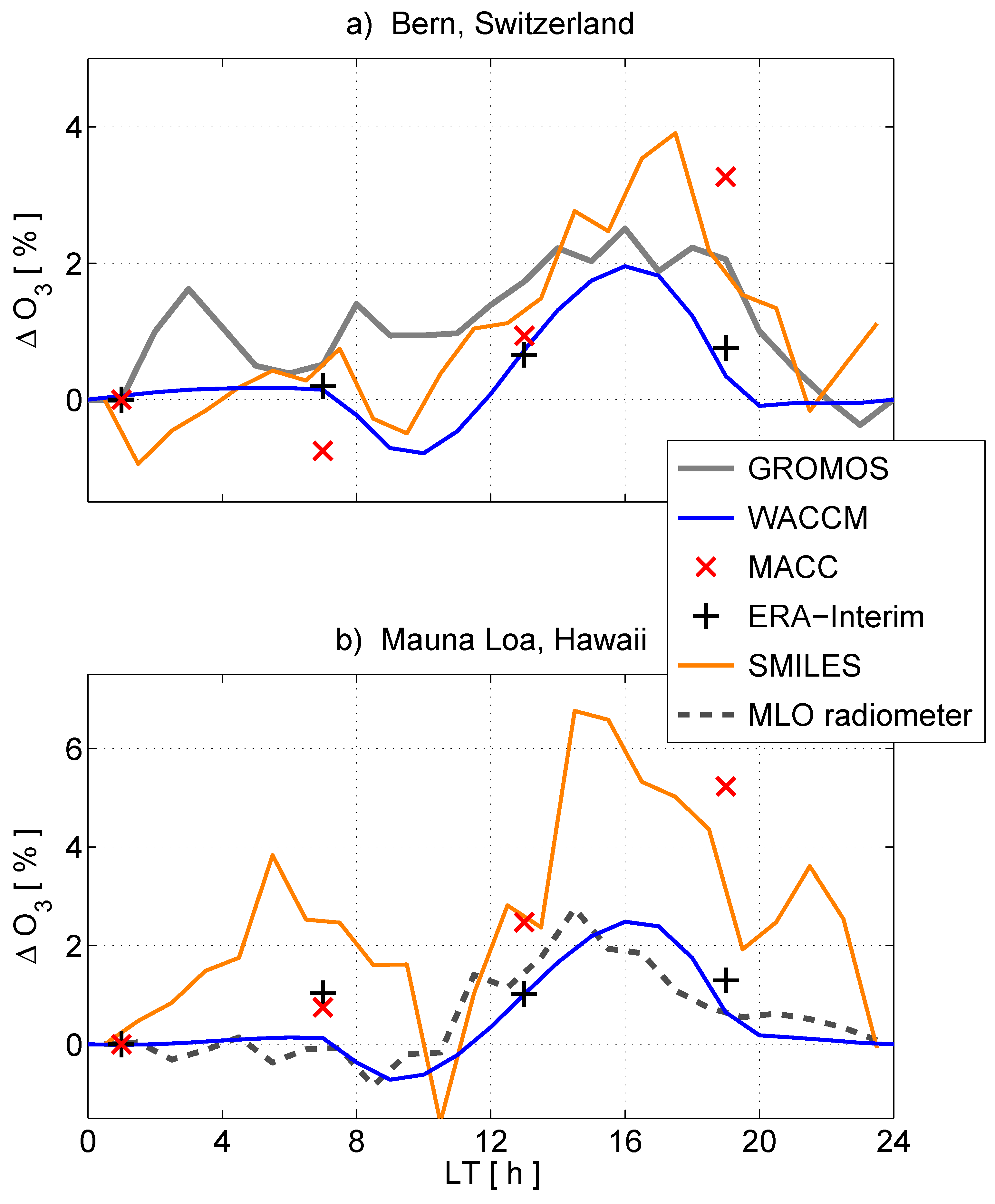
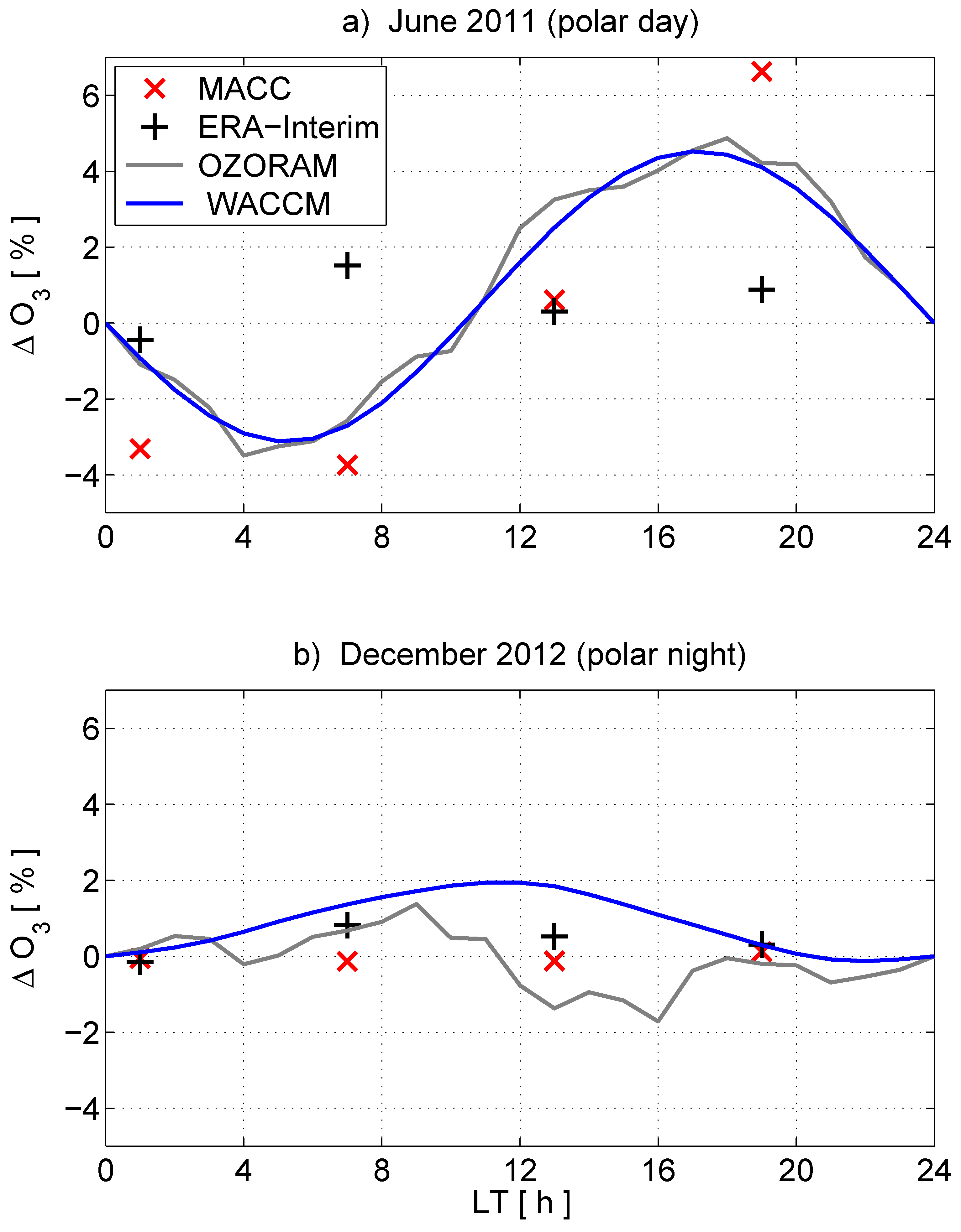
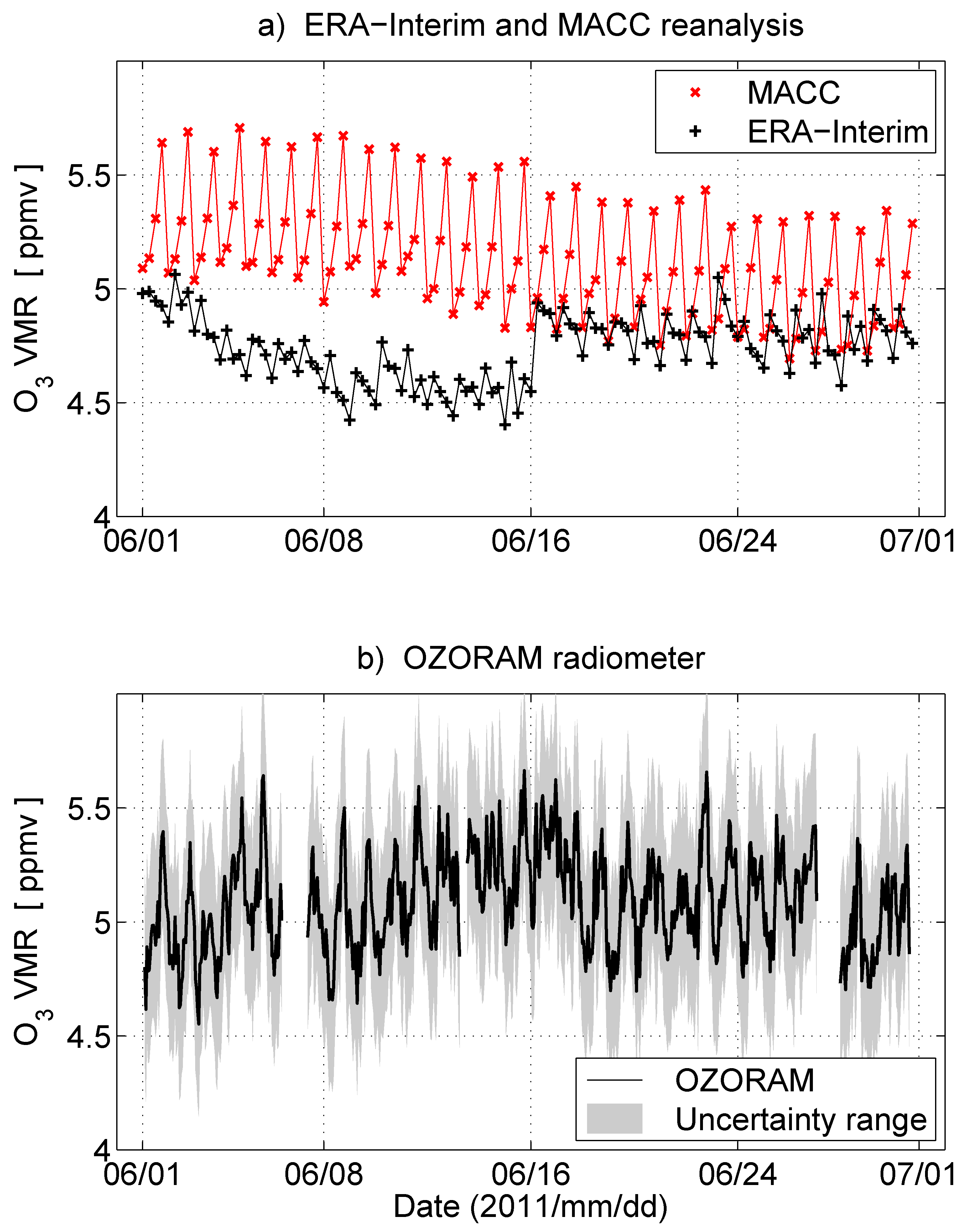
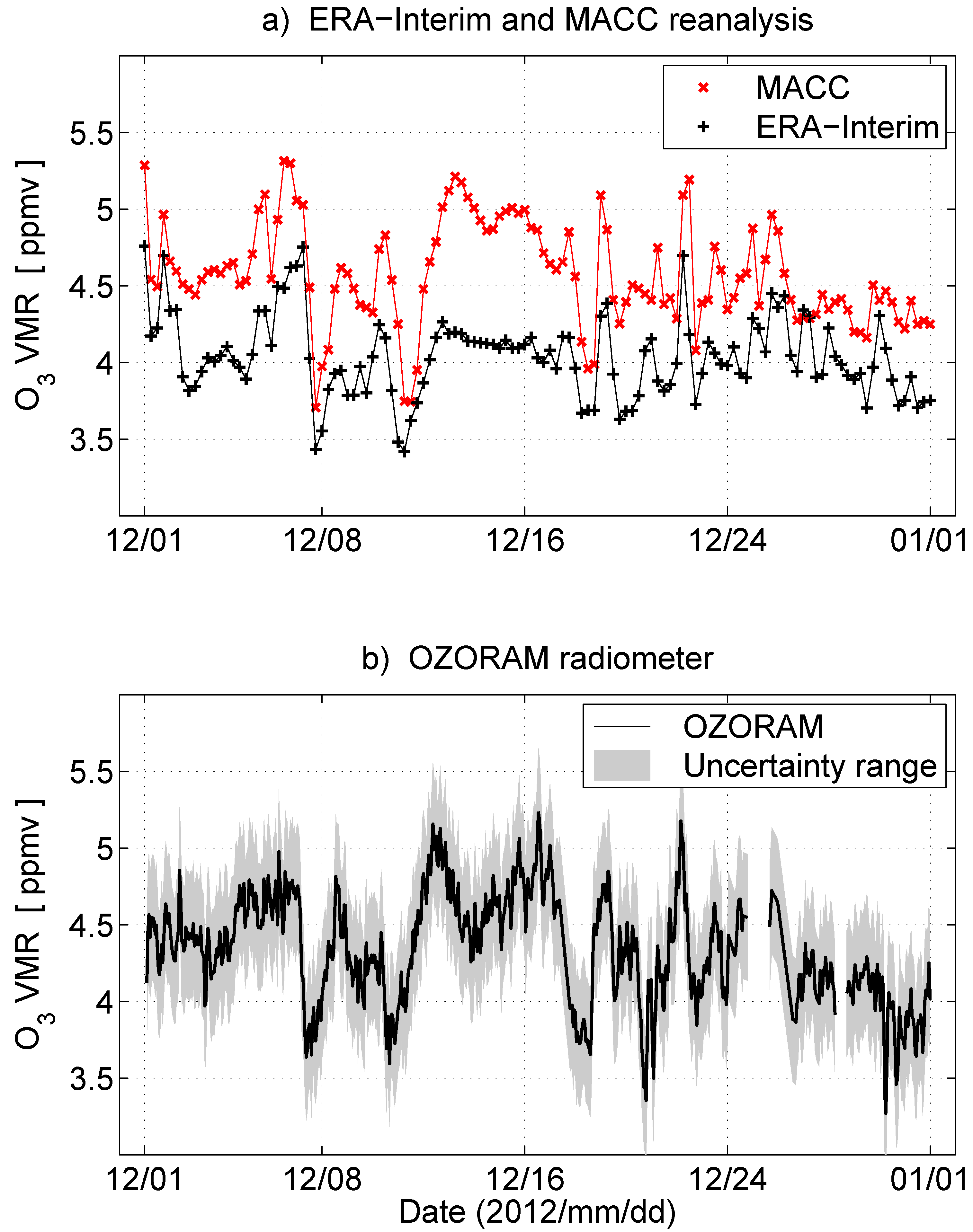
3.1. Intercomparison with Respect to Ground- and Satellite-Based Measurements

In the following diurnal ozone variation of model systems and selected NDACC sites are intercompared at the 5 hPa level which correponds to an altitude of about 38 km. At this altitude, satellite ozone trends are most biased by diurnal sampling effects due to the diurnal variation in ozone [7,14,15].
By sorting and binning of all ozone values of a month according to the local time, we get monthly mean ozone as function of local time ( O ¯ 3 ( LT ) ). The relative, diurnal ozone variation is calculated with respect to monthly mean ozone at midnight ( O ¯ 3 (0:00))
Δ O 3 ( LT ) = O ¯ 3 ( LT ) O ¯ 3 ( 0 : 00 ) O ¯ 3 ( 0 : 00 )   .
Figure 1 displays Δ O 3 ( LT ) for NDACC sites at northern midlatitudes (upper panel) and tropics (bottom panel) in March 2012. In addition to the microwave radiometers (dashed and solid gray lines), the figure comprises WACCM (blue line), MACC reanalysis (red markers), and ERA-Interim (black markers). According to Figure 1, the diurnal ozone variation at 5 hPa shows different characteristics during a day: almost constant ozone over nighttime from 22–4 LT (WACCM, MLO radiometer), a morning minimum (7–11 LT), and an afternoon maximum (14–19 LT). Table 2 compares these morning minima and afternoon maxima of the model systems and microwave radiometers. There are some differences in the occurrence time of the morning minima and afternoon maxima of the different data sets. It is clear that the temporal sampling of ERA-Interim and MACC reanalysis is not sufficient for a reliable detection of the morning minima and afternoon maxima.
There is qualitative agreement between the microwave radiometers, WACCM and MACC reanalysis (Figure 1a,b), despite the coarse temporal resolution of MACC reanalysis. At 19 LT, the Δ O 3 values of MACC reanalysis are higher than those of WACCM and the radiometers at Mauna Loa and Bern. Actually, it would be more reasonable that the coarse temporal resolution of MACC reanalysis would result in an underestimation of the diurnal ozone variation since the extrema cannot be resolved. However, it could be that small-scale variability of ozone in MACC reanalysis is misinterpreted as diurnal ozone variation. Further uncertainties might be related to the chemical data of the CTM in MACC reanalysis which is coupled every hour only. Nevertheless, the 6-hourly data of MACC reanalysis is already valuable for the study of the diurnal ozone variation on a global scale. Further progress can be expected by derivation of the diurnal ozone variation from the 3-hourly data of CAMS reanalysis. Finally, it is noticeable that ERA-Interim renders only a small diurnal variation in ozone of approximately 1%, as shown in Figure 1 and Table 2.
Further, Figure 1 includes the SMILES climatologies (orange line) for mid-latitudes (20 N to 50 N) and tropics (20 S to 20 N). For March, the SMILES product offers a bimonthly climatology of March–April only. Over Bern, Switzerland, the SMILES climatology agrees with the morning minimum and the afternoon maximum of WACCM and MACC reanalysis (see Table 2). Over Mauna Loa, Hawaii, there is only qualitative agreement of the SMILES climatology and all other data sets. It is noted that Reference [48] compiled the SMILES climatology by sampling bimonthly zonal mean profiles from non-sun-synchronous orbits, thus from all local times. The apparent discrepancy of SMILES over the Mauna Loa NDACC site (Figure 1b) may be related to the irregular data sampling due to the ISS orbit which accounts of up to 20% (relative error) in the SMILES climatology product [48]. Such discrepancies or the small phase biases in Figure 1 remind that chemical model representations and sampling frequencies of observations are imperfect or suboptimal. Nevertheless, the model systems describe the diurnal variation and it is of high interest how strong it is in the stratosphere for different altitudes, latitudes, and seasons.

3.2. Discussion of Uncertainities

This subsection has been added in 2021 for further understanding of the deviations between the different daily ozone cycles in Figure 1 and for discussion of new data analysis methods for the derivation of the diurnal ozone cycle. In the following, we focus on the diurnal ozone cycle which is present at a ground station or at a fixed model grid point. Unfortunately, it was not possible to rerun our data analysis programs from 2015, and so we cannot provide the error bars for Figure 1. As a compensation, we explain how the error bars of the diurnal ozone cycle (Equation (1)) can be derived.
There are several shortcomings in our study which can be easily avoided in future studies. The coincident model data was selected for the grid point which is nearest to the radiometer ground station. Thus, the distance between the model grid point and the sounding volume is up to 1–1.5 in latitude and longitude. In future, it would be better to interpolate the model field to the position of the sounding volume. In addition, the present study did not consider the slanted antenna beam of the radiometer which causes a distance between the geographical position of the ground station and the sounding volume. The horizontal distance is about 150 km for a 20 elevation angle of the antenna.
Further, the high-resolution ozone profiles of the models and SMILES were not adjusted by averaging kernel (AVK) smoothing to those of the ground-based radiometers which have a coarse vertical resolution of about 10 km. Reference [23] showed the effect of averaging kernel smoothing in their Figure 3. After smoothing, the daily ozone cycle of the high-resolution model is reduced by about 10% in the stratosphere from 30–2 hPa (25–45 km), and the maximum of the diurnal ozone amplitude is shifted from 4 hPa to 5.5 hPa (ca. 2–3 km decrease in height). Larger effects of AVK smoothing occur above 2 hPa (45 km). Since it is a pity to degrade the information content of high-resolution profiles, one should consider to provide both, the original and the smoothed results. Another point is to investigate if the daily ozone cycle depends more strongly on the solar zenith angle than on local time and if the daily ozone cycle should be shown as function of solar zenith angle. In case of SMILES, the deviations in Figure 1 can be due to a lack of spatial and temporal coincidence. Contrary to MACC, ERA-Interim and the ground stations, the SMILES curves were derived for a different year (2010 instead of 2012) and for the March/April period instead of March. Further, zonal means of broad belts were taken, while the ground stations lay at the edges of the belts. The level 2 climatology data sets were provided by the SMILES mission team. It is hard to estimate if better results could be achieved by a new data analysis of SMILES level2 data, which would be designed for our special purposes. Generally, it is a good idea to compare the diurnal ozone cycle from a ground station to zonal means of satellites or models since the effect of small-scale variability in the regional ozone data will be reduced. In case of the GROMOS results in Figure 1a), it should be stated that the ozone profile retrieval of GROMOS had some shortcomings. At the moment, the Institute of Applied Physics develops a complete new retrieval for GROMOS at Bern and the Stratospheric Ozone Monitoring Radiometer (SOMORA) at Payerne. These microwave radiometers are close together (ca. 40 km distance), and since 2009 both radiometers are equipped with similar FFT spectrometers. In the new retrieval, the data quality control and the error analysis are optimized leading to an improved vertical resolution. The forward model of the inversion correctly takes into account the effect of the tropospheric opacity on the spectrum. We are going to check if the daily ozone cycle can be better captured by the new retrieval applied to the radiometer datasets at Bern and Payerne. Reference [23] provided error bars of about ± 2 % for the mean diurnal ozone cycles in the stratosphere in their Figure 6. They analyzed a 17-year time interval of GROMOS spectra which were recorded with a digital filter bench. A digital filter bench is certainly not so reliable and stable as a FFT spectrometer. The derivation of the error of the mean was simple: Reference [23] had 17 daily ozone cycles for each month (e.g., 17 January months from 1995 to 2011). Then, they calculated the standard deviation of the 17 curves, and the error of the mean is equal to the standard deviation divided by 17 . Reference [15] derived error bars of about ± 1 % for the difference between day- and nighttime ozone in the stratosphere coincidently measured by the MLO radiometer, SMILES and EOS-MLS Aura using observations from October 2009 to April 2010 (e.g., their Figure 5). The deviations between the instruments were within their error bars. Now, we derive the formula for the error bars for Equation (1). The standard deviations of the monthly means O ¯ 3 ( LT ) and O ¯ 3 (0:00) are
σ 1 = 1 n 1 i = 1 n ( O 3 , i ( LT ) O ¯ 3 ( LT ) ) 2 ,
σ 2 = 1 n 1 i = 1 n ( O 3 , i ( 0 : 00 ) O ¯ 3 ( 0 : 00 ) ) 2 ,
where n is the number of the days of a month. The errors of the means are
σ m , 1 = σ 1 n and σ m , 2 = σ 2 n .
Applying Gaussian error propagation to Equation (1), we get the total error σ ( LT ) of the relative diurnal ozone cycle Δ O 3 ( LT )
σ ( LT ) = σ m , 1 2 O ¯ 3 ( 0 : 00 ) 2 + O ¯ 3 ( LT ) 2 O ¯ 3 ( 0 : 00 ) 4 σ m , 2 . 2
Equation (5) should be used for the calculation of the missing error bars in Figure 1. For a discussion, a rough approximation of Equation (5) might be useful assuming σ m , 2 σ m , 1 and O ¯ 3 (0:00) ≈ O ¯ 3 (LT), which leads to
σ ( LT ) 2 σ m , 1 O ¯ 3 ( LT ) .
The uncertainty σ ( LT ) can be reduced by analyzing longer time intervals since the error of the mean σ m , 1 will decrease if more months are taken in the analysis. The error of the mean is influenced by different factors which can be due to measurement and retrieval errors, small-scale ozone variability, planetary wave-like oscillations, seasonal gradients in ozone, and possible interannual variability of the diurnal ozone variation. One idea is to reduce the disturbing influence of planetary wave-like oscillations by high pass-filtering of the ozone time series observed or modeled at a certain location, so that the diurnal variation is separated from the planetary wave-like oscillations and the seasonal gradient. The filtered ozone series is then used for the derivation of the daily ozone cycle. However, the method should be tested by means of artificial time series.
For ground stations, the small-scale variability is the most serious problem, e.g., ozone laminae can drift through the sounding volume, enhancing σ m , 1 and generating a bias of the derived daily ozone cycle. The four beam-radiometer GROMOS-C [55] led to a progress in the study of small-scale variability of middle-atmospheric ozone. GROMOS-C permanently sounds in East, West, North, and South direction with a horizontal range of about 150 km around the station. The intercomparison of the strengths and directions of horizontal ozone gradients measured by GROMOS-C and coincidently simulated by models showed that SD-WACCM and MERRA-2 can capture the observed small-scale variability [55]. Finally, it can be stated that both kinds of diurnal ozone cycle are interesting for research: a smooth zonal mean diurnal ozone cycle, as well as a temporally intermittent, regional variable diurnal ozone cycle. In practice, it is difficult to mark a boundary.

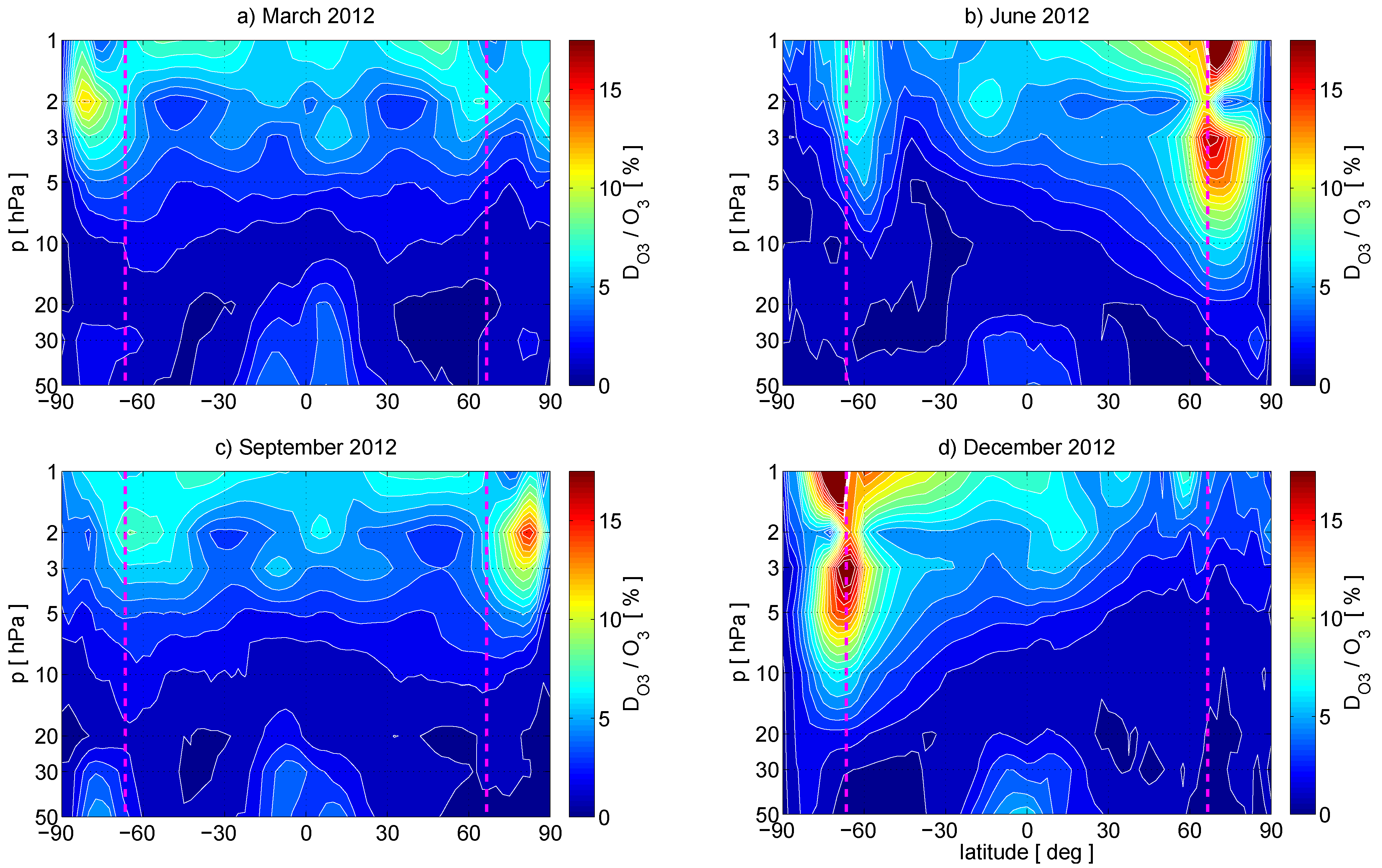
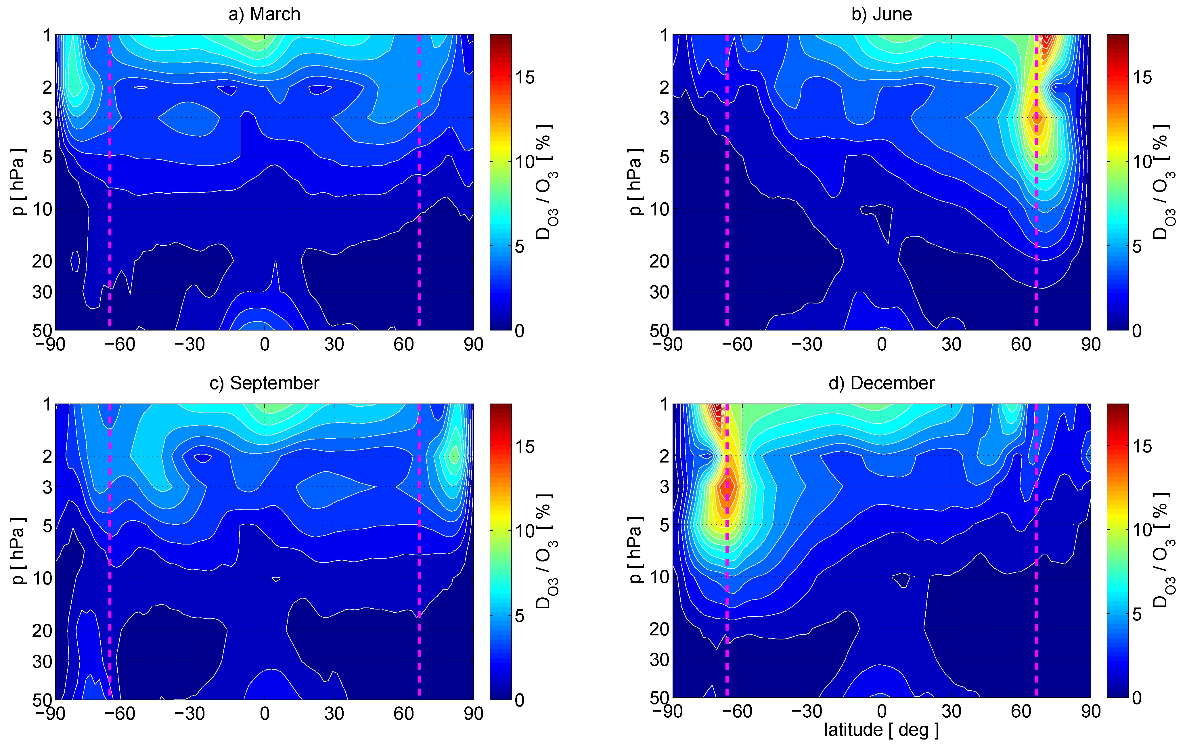
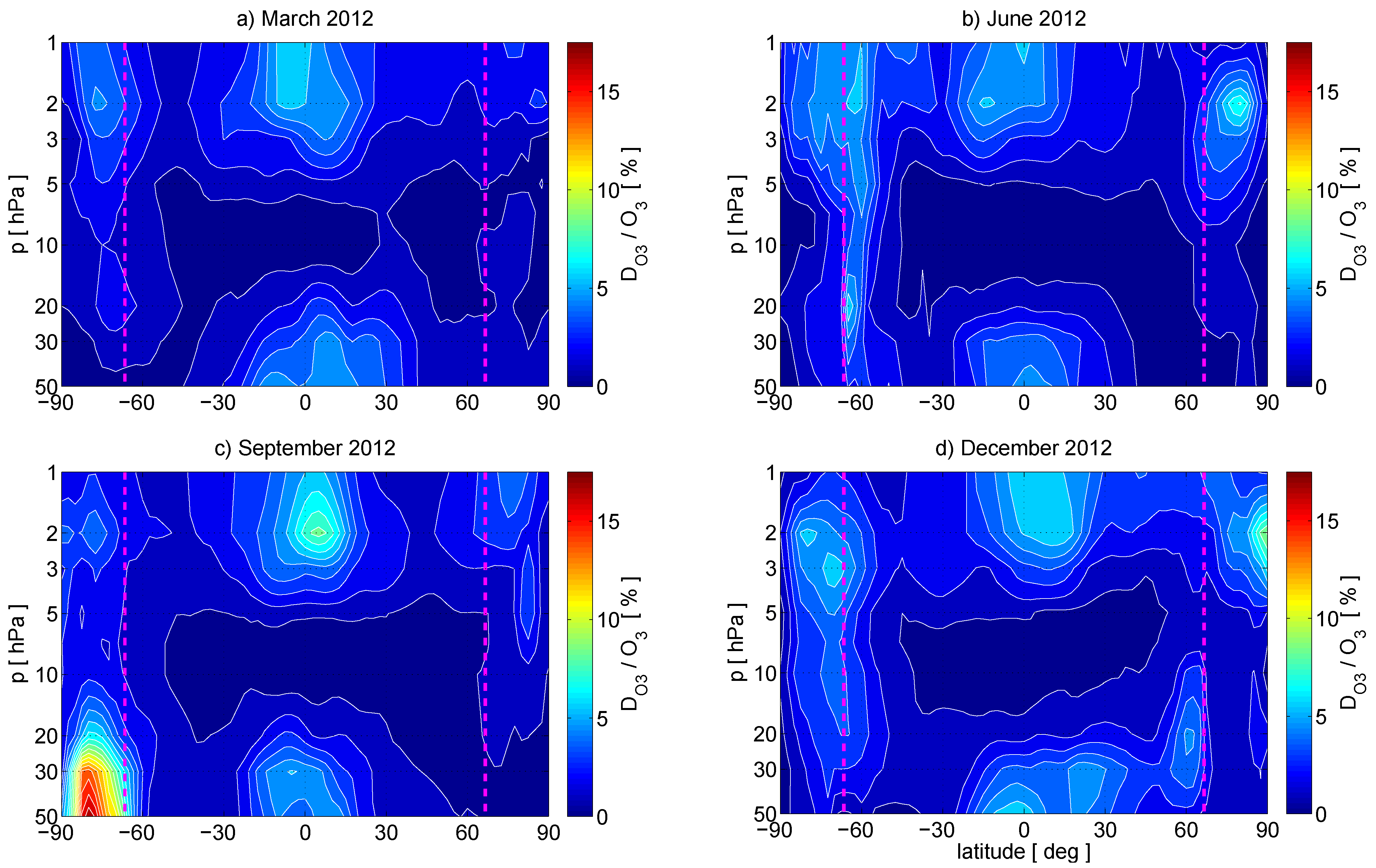
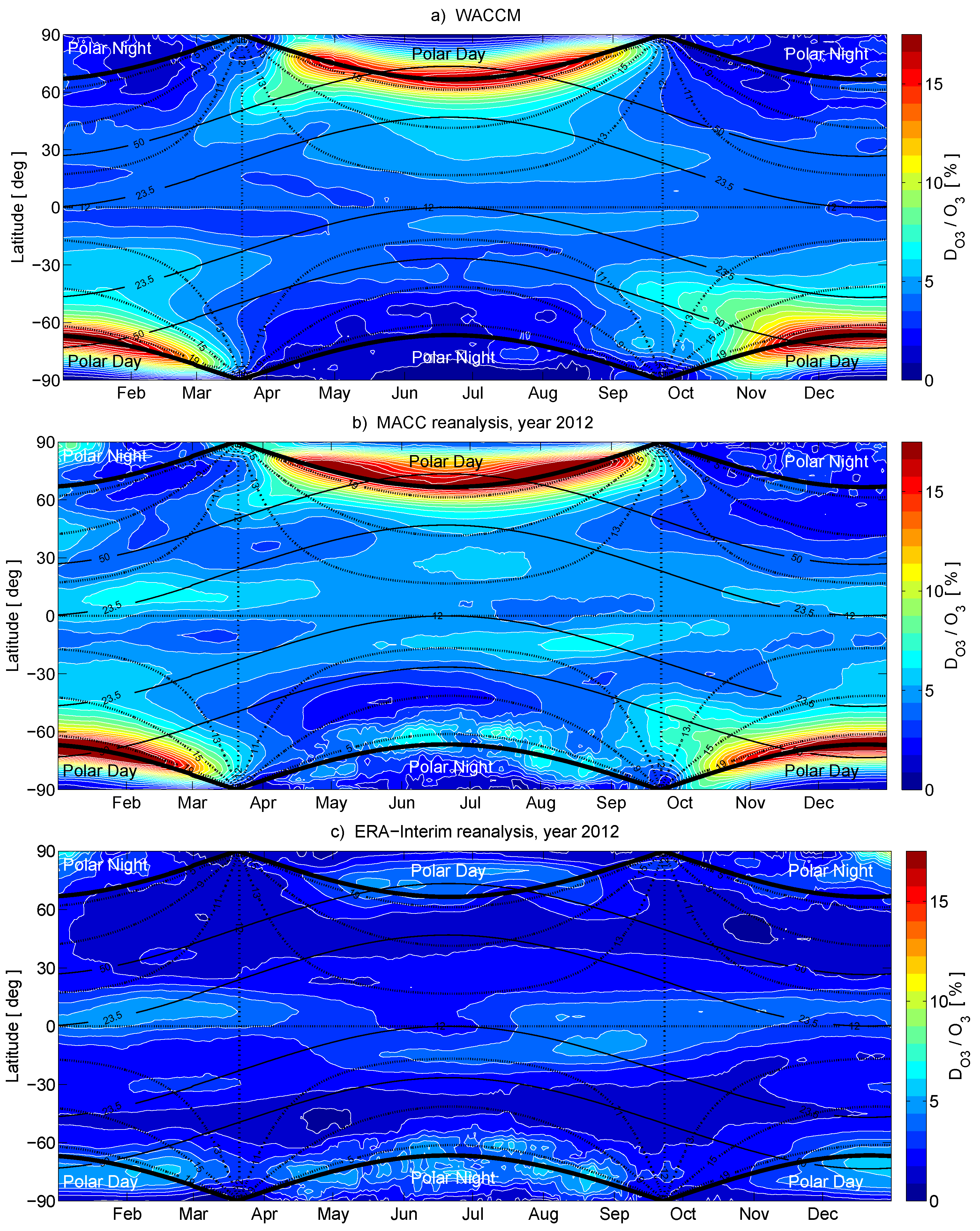
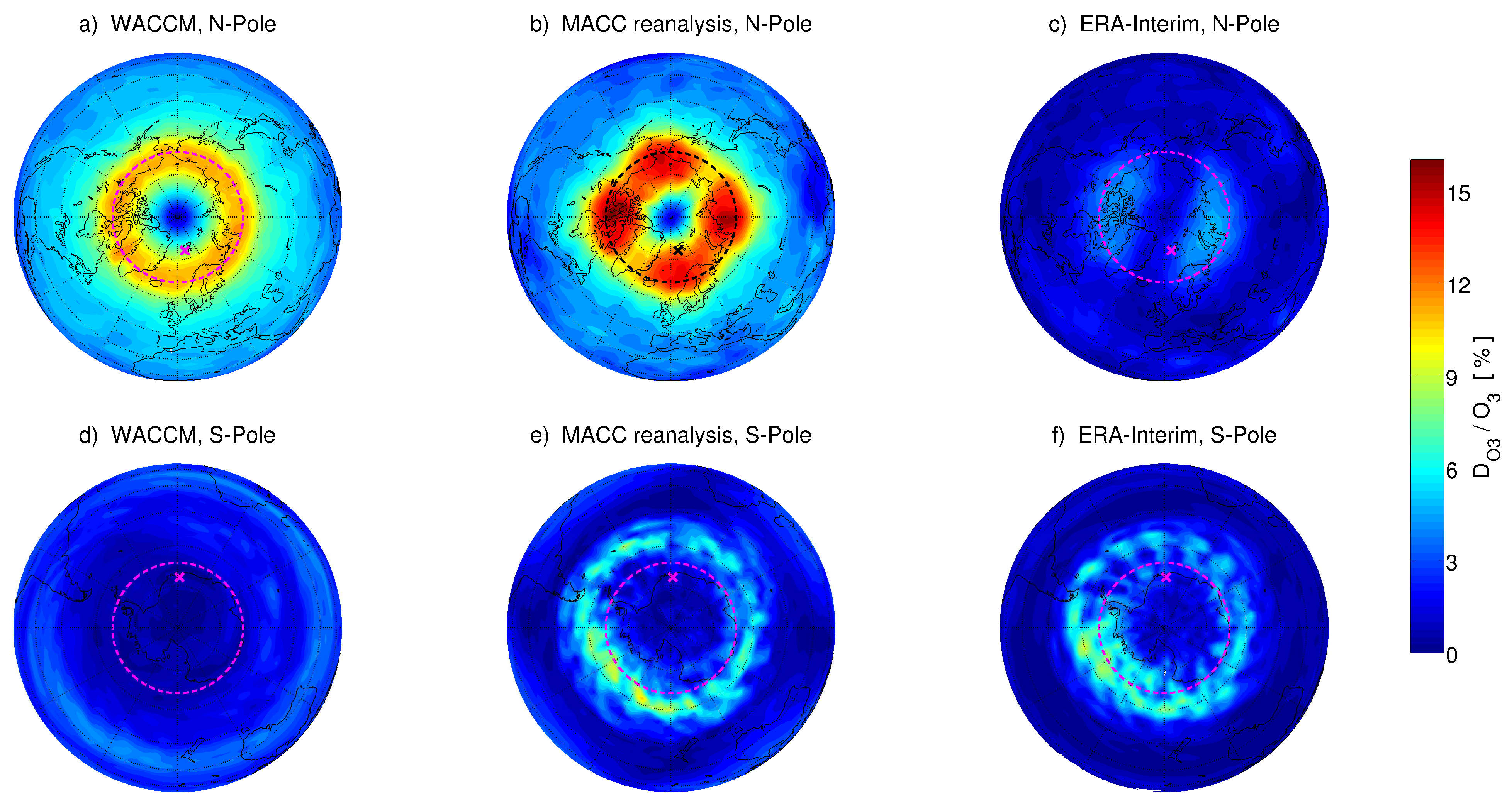
3.3. Intercomparison of the Model Systems

For the global analysis of the model systems the diurnal variation was deduced without the small disturbances from, e.g., subseasonal variations or synoptic eddies. This was achieved by subtracting a 24-h running mean from the time series. The residual diurnal variation was then sorted and binned by universal time to a monthly mean diurnal variation as function of universal time ( Δ O ¯ 3 ( UT ) ). The strength of the diurnal variation in ozone is represented by the peak-to-valley difference D O 3 , which is deduced according to Equation (7) at each grid point.
D O 3 = max { Δ O ¯ 3 ( UT ) } min { Δ O ¯ 3 ( UT ) . }
We discuss this peak-to-valley difference in relative units D O 3 /O3, where O 3 is monthly mean ozone at a grid point.
Figure 2 shows zonal-mean D O 3 /O3 for March, June, September and December of 2012 from MACC reanalysis. The strengths of the diurnal ozone variation is presented over latitude for the pressure range from 1 to 50 hPa. Figure 2a,c displays substantial diurnal ozone variation above the 5 hPa pressure level and below 20 hPa in the tropics (20 S–20 N) in March and September. In the lower, tropical stratosphere (15–50 hPa) the diurnal variation originates from dynamics. In this region vertical tidal winds transport odd oxygen ( Ox ) along a strong vertical ozone gradient, which leads to a diurnal variation [14]. In the middle stratosphere (2.5–15 hPa) the diurnal variation of ozone is driven by insolation and leads to specific characteristics as in Figure 1 at 5 hPa. In a broad sense, the morning minimum results from a fast ozone loss due to activated NO and Cl radicals after sunrise. During daytime ozone is rebuilt and accumulated to an afternoon maximum by reactions of the Chapman cycle (cf. Figure 1). For a detailed discussion of the diurnal ozone budget at 5 hPa, we refer to Reference [17]. In the upper tropical stratosphere (1–2.5 hPa), the diurnal variation is caused by a mix of both, photochemistry and dynamics [14].
In the MACC reanalysis data, the diurnal variation of stratospheric ozone is enhanced in June and December at the Arctic and Antarctic polar circles (marked as magenta dashed lines). For instance, in Figure 2b,d, MACC reanalysis shows high values of diurnal ozone variation of up to 17% (1.6 ppmv) in the respective summer hemisphere between 5 hPa (38 km) and the stratopause at 1 hPa (50 km). The effect is generated by the long sunshine duration at the polar circle in summer which results in a strong ozone accumulation during daytime. This feature was described and explained by Reference [17] for the 5 hPa pressure level only. The MACC reanalysis shows that the enhanced diurnal variation occurs over a wide vertical and horizontal range with the maximum at 3 hPa.
Surprisingly, MACC reanalysis indicates a diurnal variation in domains where the insolation is negligible or not existing. These regions are the polar regions in winter. The upper stratosphere (3–1 hPa, 40–50 km) in June has a diurnal variation in ozone of up to 8% (0.8 ppmv) near the Antarctic polar circle, as shown in Figure 2b. The Antarctic stratosphere in winter is a dynamically dominated region and most of this diurnal ozone variation must relate to diurnal advection effects. To the authors knowledge, this feature of ozone variability at diurnal time scale is a novelty and has not been reported yet.
In a similar manner, Figure 3 displays D O 3 /O3 for March, June, September and December from the WACCM simulation. In order to have the same temporal resolution as MACC reanalysis and ERA-Interim, the hourly WACCM output was down-sampled to 6 h. In the WACCM simulation the diurnal variation of stratospheric ozone is maximal in June and December at the polar circle of the summer hemisphere between the stratopause and 5 hPa. This strong diurnal variation of up to approximately 14% (0.8 ppmv) can be clearly seen in Figure 3b,d. These features are mostly consistent with the results of MACC reanalysis. Only a small difference occurs in the peak strengths which are slightly higher for MACC reanalysis. Further, the diurnal variation in the lower, tropical stratosphere is very weak in WACCM. In this context, it is important to note that the WACCM simulation was free-running without any nudging or data assimilation. When model dynamics are nudged, also WACCM can describe this dynamical effect in the lower, tropical stratosphere SD-WACCM, [14].
Generally, WACCM and MACC reanalysis show very similar diurnal ozone variation from the stratopause to 10 hPa with one major exception. Compared to MACC reanalysis, WACCM shows little or no diurnal variation at the Antarctic polar circle in winter (cf. Figure 2b and Figure 3b). This region, the winter stratosphere, is dominated by dynamics. As for the lower stratosphere the bias to MACC reanalysis seems to be related to dynamics at diurnal time scales which are less distinct in the free-running WACCM.
The last model system, ERA-Interim, is often used and well-recognized in atmospheric sciences. D O 3 / O 3 from ERA-Interim is presented in a similar manner as for the other model systems in Figure 4. ERA-Interim shows considerably less diurnal variation in ozone from the stratopause to 10 hPa. We infer that this is to a wide extent a result of the coefficients of the linear ozone scheme which are not a function of longitude [35]. A further cause might be that ERA-interim considers only a one-way coupling from dynamics to ozone (see Table 1). The apparent diurnal variation above 10 hPa might partly originate from assimilated ozone data with a diurnal sampling. However, there exist periods of the reanalyses where ozone has been assimilated from sun-synchronous satellites only May–July 2004, [25]. During this period without diurnal sampling, the diurnal variation is similar to the results of the present study. We infer that the diurnal variation of the two reanalysis model systems mostly comes from the calculated diurnal advection and the coupled CTM or ozone scheme and not from the assimilated ozone data.
Finally, ERA-Interim mostly agrees to the diurnal variation in ozone of MACC reanalysis in the lower, tropical stratosphere. The surprisingly strong diurnal variation at the Antarctic polar circle occurs also in ERA-Interim. It accounts for up to 7% (0.5 ppmv). Both features are present in the reanalyses with 4-D-VAR data assimilation only and not in the free-running WACCM. This strongly suggests a dynamical origin of the intriguing effect at the Antarctic polar circle.
According to Figure 2, Figure 3 and Figure 4, there are substantial seasonal changes in the behavior of the diurnal variation in stratospheric ozone. Figure 5 presents this seasonal behavior of the diurnal ozone variation of the three model systems at 3 hPa. The presented continuous monthly mean is achieved by a sliding time window of ± 15 days. The resulting 30 days period is analyzed with the method described by Equation (7). Contours in Figure 5 depict the sunshine duration (dashed lines) and the solar zenith angle (solid lines). It can be seen that neither WACCM nor ERA-Interim show all the characteristics which we inferred from MACC reanalysis. The strong diurnal variation in ozone caused by a photochemical variation is established during summer near the polar circle. ERA-Interim mostly misses this feature. On the other hand, the diurnal variation in the Antarctic polar winter stratosphere is an intermittent feature at the edge of the polar vortex which is not modeled by the free-running WACCM.
The three model systems show different features of the diurnal variation in ozone according to their specific model compositions. The apparent disagreements in the diurnal photochemical variation or short-term advection of WACCM and ERA-Interim strongly suggest different origins of the diurnal ozone variation in the stratosphere. The MACC reanalysis combines data assimilation with a strong chemical representation module and gives an unprecedented global picture on diurnal ozone variation in the stratosphere.

3.4. Diurnal Variation in the Arctic and Antarctic

The strong diurnal variation in the Arctic region is accessible by measurements of the NDACC network. The measurements of OZORAM (78.9 N, 11.9 E) confirm the diurnal ozone variation of MACC reanalysis at Ny-Ålesund which is strong in summer and non-existent in winter.
Figure 6a presents the mean diurnal variation in ozone as observed by OZORAM in June 2011 at 5 hPa. Further, the figure shows the corresponding data of MACC reanalysis, ERA-Interim and WACCM at Ny-Ålesund. The diurnal variation in ozone Δ O 3 ( LT ) is deduced according to the definition of Equation (1). The diurnal ozone variation at Ny-Ålesund is up to approximately 8% for WACCM and OZORAM in summer which are almost perfectly consistent. The MACC reanalysis has a slightly stronger diurnal variation in ozone at Ny-Ålesund of up to 10%, while ERA-Interim shows only a small variation of 2% in June 2011. The sensed profiles of OZORAM agree with MACC reanalysis and WACCM also at higher altitudes of the stratosphere, which is not shown. In addition, Figure 7a shows the ozone time series for June 2011 of MACC reanalysis, ERA-Interim and from the OZORAM observations. One can clearly see that MACC reanalysis and the OZORAM measurements are consistent for the diurnal variation and the ozone VMR, while ERA-Interim underestimates the measured diurnal variation and to some extent the ozone VMR over Ny-Ålesund. Further, ERA-Interim shows a sudden increase at 16 June 2011 over Ny-Ålesund with no equivalent in the OZORAM measurements.
Similarly, Figure 6b and Figure 8b display the diurnal variation and the corresponding time series for December 2012 of OZORAM and the model systems. All the model systems show a maximal diurnal variation of less than 2% for this period in winter (polar night). This almost negligible diurnal variation is confirmed by the OZORAM observations. As shown by the ozone time series in December 2011 in Figure 8 there is no signal of a diurnal variation in ozone at 3 hPa. The December 2012 ozone series of MACC reanalysis and OZORAM agree well within the combined error range of the radiometer measurements, while ERA-Interim tends to indicate less ozone as in summer 2011. However, the dynamically dominated polar region in winter does not show a diurnal variation in the Arctic over Ny-Ålesund, Svalbard.
In the southern hemisphere, MACC reanalysis and ERA-Interim indicate a diurnal variation during Antarctic winter of approximately 8% at the polar circle (see Figure 2b and Figure 4b). During the polar night, photochemical variations are negligible so that dynamics are considered as the origin of this diurnal variation in ozone. A view on the diurnal ozone variation with focus on the Arctic and Antarctic is presented in Figure 9 for the three model systems. The figure presents the peak-to-valley difference corresponding to Equation (7) on the northern and southern hemisphere for June 2012. Thus, the upper panels describe Arctic summer (polar day) and the lower panels Antarctic winter (polar night) situations, respectively. In the northern hemisphere the magenta markers indicate the geographical location of OZORAM at Ny-Ålesund, Svalbard. Figure 9a,b displays the strong diurnal variation in the Arctic summer which was locally confirmed by OZORAM (see marker for Ny-Ålesund). Compared to WACCM and MACC, ERA-Interim shows too little diurnal variation in this region (Figure 9c). In Figure 9e,f, the reanalysis systems MACC and ERA-Interim consistently show an enhanced diurnal ozone variation in the polar winter stratosphere around the Antarctic from about 50–70 S, while WACCM completely misses this feature in the Antarctic.
The NDACC network does not operate a ground-based ozone radiometer in the Antarctic. There exist measurements of the British Antarctic Survey’s ground-based Microwave Radiometer at Troll (BAS-MRT), Antarctica (72 01 S, 02 32 E) from February 2008 and throughout January 2010 [56]. The ozone profiles are sensed over Troll from 0.02 to 3 hPa (see markers in the lower panels of Figure 9). These observations might be valuable for exploration of the diurnal ozone variation in the Antarctic.
The enhanced diurnal ozone variation at latitudes from 50–70 S (along the Antarctic polar circle) of MACC and ERA-Interim is intriguing and seems to be related to dynamics. The Antarctic polar vortex is a strong mixing barrier in the stratosphere and establishes strong ozone gradients which foster ozone variations by horizontal and vertical advection. In local time series of the MACC reanalysis and ERA-Interim we found that this effect is intermittent and less sustained compared to the photochemical variation in summer (cf. Figure 7). A possible cause of the diurnal ozone variation might be a diurnal elongation and displacement of the vortex [57].

4. Conclusions

We intercompared the diurnal variation in ozone from reanalysis and chemistry–climate modeling and presented a wide range of agreements but also discrepancies. For instance, the strong diurnal variation in ozone at the polar circles in summer appear similar in MACC reanalysis and WACCM. We confirmed this effect by measurements of the OZORAM radiometer in the high Arctic at Ny-Ålesund. Generally, earlier studies described the diurnal variation in stratospheric ozone as a result of ozone accumulation due to the Chapman cycle over day time which is not entirely balanced by catalytic ozone depletion. We find that ERA-Interim with its linearized, two-dimensional photochemical ozone model underestimates such a diurnal variation in stratospheric ozone caused by a photochemical variation. Differences also appear when the diurnal variation is caused by dynamics. The free-running WACCM shows less diurnal variation than MACC reanalysis and ERA-Interim in the lower, tropical stratosphere where the diurnal variation emerges from tidal winds and a strong ozone gradient. Further, MACC reanalysis and ERA-Interim indicate dynamically originated diurnal variations of up to 8% in the Antarctic stratosphere at the edge of the polar vortex. We find that the two reanalysis model systems show a good dynamical representation of the stratosphere and these indicated diurnal variation might be real. However, this needs further investigation with diurnally sampled observations of the Antarctic stratosphere to finally confirm such diurnal variations in ozone.
The comparison to ERA-Interim and WACCM substantiates the benefits of a coupled CTM for the representation of the diurnal variation in stratospheric ozone as implemented in the MACC reanalysis system. Our intercomparison study indicates the potential of MACC reanalysis to accurately describe the diurnal variation of stratospheric ozone while ERA Interim and the free-running WACCM have weaknesses in the representation of either photochemically or dynamically induced diurnal variations. The higher temporal resolution of CAMS reanalysis compared to MACC reanalysis will allow improved studies about the daily ozone cycle.
In addition, the results show how gathering and preparation of data by the affiliated ground stations of the NDACC network yields additional value for atmospheric research and the validation of the MACC reanalysis model system. Ground-based microwave radiometry is an important observation method for the diurnal variation of stratospheric ozone. Partly, it was possible to validate the different model systems by NDACC observations. Therefore, further measurements of diurnal ozone variation in the polar regions as performed by Reference [18] are desirable to confirm and study the behavior of diurnal variation in ozone at different seasons in the Arctic and Antarctic. For instance, the start-up of the campaign instrument GROMOS-C [58] makes polar stratospheric ozone and its diurnal variation more accessible to ground-based microwave radiometry and extends the global sampling of local ozone profiles. Reference [59] analyzed the diurnal variation in middle-atmospheric ozone measured by GROMOS-C at Ny-Ålesund in 2015/2016. Their results are in agreement with the present study though the maximal amplitude of the daily ozone cycle is about 13% at 3 hPa in April 2016 [59]). The measurements of GROMOS-C at Ny-Ålesund are continued up to now (April 2021), so that the derivation of a climatology of the daily ozone cycle at Ny-Ålesund is possible.
Despite a suboptimal temporal resolution, the MACC reanalysis system impressively showed dynamical and photochemical features of diurnal variation in ozone at all latitudes and seasons. On this account, such a model system of chemical data integration and assimilated dynamics shows great promise for preprocessing diurnally sampled ozone data from space-borne instruments and correct potential biases in ozone trends. The diurnally sampled observations might be assimilated and reanalyzed with a coupled chemical transport model under consideration of a higher temporal resolution.

Author Contributions

Conceptualization, A.S.; methodology, A.S and K.H.; software, A.S.; validation, all; formal analysis, A.S.; investigation, all; resources, all; data curation, all; writing—original draft preparation, A.S.; writing—review and editing, all; visualization, A.S.; supervision, K.H. and N.K.; project administration and funding acquisition, K.H. and N.K.; final manuscript revision, K.H. All authors have read and agreed to the published version of the manuscript.

Funding

The research leading to these results has received funding from the European Community’s Seventh Framework Program (FP7/2007–2013) under grant agreement NO 284421 (see Article II.30. of the Grant Agreement). The OZORAM measurements at the AWIPEV research base have been supported by the AWI Bremerhaven and the Deutsche Forschungsgemeinschaft (DFG) in the projects NO 404/5-1, NO 404/5-2, NO 404/5-3.

Data Availability Statement

OZORAM and GROMOS data are at https://www.ndacc.org. SMILES data are at https://smiles.nict.go.jp/index-e.html, and WACCM simulation data can be requested. MACC and ERA data are at https://www.ecmwf.int (all accessed on 12 May 2021).

Acknowledgments

We acknowledge the MACC-II consortium, ECMWF for access to ERA-Interim data, the International Space Science Institute at Bern, Switzerland (ISSI Team 246, Characterizing Diurnal Variations of Ozone for Improving Ozone Trend Estimates, http://www.issibern.ch/teams/ozonetrend/, accessed on 12 May 2021 and the MeteoSwiss project MIMAH in the frame of GAW. We thank the AWI Bremerhaven for logistic support on the AWIPEV station and the station personnel in Ny Ålesund, Spitsbergen. We gratefully acknowledge the funding by DFG Project-ID 268020496 TRR 172, within the Transregional Collaborative Research Center “ArctiC Amplification: Climate Relevant Atmospheric and SurfaCe Processes, and Feedback Mechanisms (AC)3”, subproject E02. We also acknowlegde support by the Senate of Bremen, Germany. Further, we thank Lorena Moreira for consultations on GROMOS data. We thank the reviewers for their efforts and corrections.

Conflicts of Interest

The authors declare no conflict of interest.

References

  1. Schanz, A.; Hocke, K.; Kämpfer, N.; Chabrillat, S.; Inness, A.; Palm, M.; Notholt, J.; Boyd, I.; Parrish, A.; Kasai, Y. The diurnal variation in stratospheric ozone from the MACC reanalysis, the ERA-Interim reanalysis, WACCM and Earth observation data: Characteristics and intercomparison. Atmos. Chem. Phys. Discuss. 2014, 14, 32667–32708. [Google Scholar] [CrossRef] [Green Version]
  2. Frith, S.M.; Bhartia, P.K.; Oman, L.D.; Kramarova, N.A.; McPeters, R.D.; Labow, G.J. Model-based climatology of diurnal variability in stratospheric ozone as a data analysis tool. Atmos. Meas. Tech. 2020, 13, 2733–2749. [Google Scholar] [CrossRef]
  3. Hersbach, H.; Bell, B.; Berrisford, P.; Hirahara, S.; Horányi, A.; Muñoz-Sabater, J.; Nicolas, J.; Peubey, C.; Radu, R.; Schepers, D.; et al. The ERA5 global reanalysis. Q. J. R. Meteorol. Soc. 2020, 146, 1999–2049. [Google Scholar] [CrossRef]
  4. Gelaro, R.; Mccarty, W.; Suárez, M.J.; Todling, R.; Molod, A.; Takacs, L.; Randles, C.A.; Darmenov, A.; Bosilovich, M.G.; Reichle, R.; et al. The Modern-Era Retrospective Analysis for Research and Applications, Version 2 (MERRA-2). J. Clim. 2017, 30, 5419–5454. [Google Scholar] [CrossRef] [PubMed]
  5. Brakebusch, M.; Randall, C.E.; Kinnison, D.E.; Tilmes, S.; Santee, M.L.; Manney, G.L. Evaluation of whole atmosphere community climate model simulations of ozone during Arctic winter 2004–2005. J. Geophys. Res. Atmos. 2013, 118, 2673–2688. [Google Scholar] [CrossRef]
  6. Inness, A.; Ades, M.; Agustí-Panareda, A.; Barré, J.; Benedictow, A.; Blechschmidt, A.-M.; Dominguez, J.J.; Engelen, R.; Eskes, H.; Flemming, J.; et al. The CAMS reanalysis of atmospheric composition. Atmos. Chem. Phys. Discuss. 2019, 19, 3515–3556. [Google Scholar] [CrossRef] [Green Version]
  7. Bhartia, P.K.; McPeters, R.D.; Flynn, L.E.; Taylor, S.; Kramarova, N.A.; Frith, S.; Fisher, B.; Deland, M. Solar Backscatter UV (SBUV) total ozone and profile algorithm. Atmos. Meas. Tech. 2013, 6, 2533–2548. [Google Scholar] [CrossRef] [Green Version]
  8. Jonsson, A.I.; Fomichev, V.I.; Shepherd, T.G. The effect of nonlinearity in CO2 heating rates on the attribution of stratospheric ozone and temperature changes. Atmos. Chem. Phys. 2009, 9, 8447–8452. [Google Scholar] [CrossRef] [Green Version]
  9. Garny, H.; Bodeker, G.E.; Smale, D.; Dameris, M.; Grewe, V. Drivers of hemispheric differences in return dates of mid-latitude stratospheric ozone to historical levels. Atmos. Chem. Phys. Discuss. 2013, 13, 7279–7300. [Google Scholar] [CrossRef] [Green Version]
  10. Chehade, W.; Burrows, J.P.; Weber, M. Total ozone trends and variability during 1979–2012 from merged datasets of various satellites. Atmos. Chem. Phys. 2014, 14, 7059–7074. [Google Scholar] [CrossRef] [Green Version]
  11. Kyrölä, E.; Laine, M.; Sofieva, V.; Tamminen, J.; Päivärinta, S.-M.; Tukiainen, S.; Zawodny, J.; Thomason, L. Combined SAGE II–GOMOS ozone profile data set for 1984–2011 and trend analysis of the vertical distribution of ozone. Atmos. Chem. Phys. Discuss. 2013, 13, 10645–10658. [Google Scholar] [CrossRef] [Green Version]
  12. Gebhardt, C.; Rozanov, A.; Hommel, R.; Weber, M.; Bovensmann, H.; Burrows, J.P.; Degenstein, D.; Froidevaux, L.; Thompson, A.M. Stratospheric ozone trends and variability as seen by SCIAMACHY from 2002 to 2012. Atmos. Chem. Phys. Discuss. 2014, 14, 831–846. [Google Scholar] [CrossRef] [Green Version]
  13. Kramarova, N.A.; Frith, S.M.; Bhartia, P.K.; McPeters, R.D.; Taylor, S.L.; Fisher, B.L.; Labow, G.J.; DeLand, M.T. Validation of ozone monthly zonal mean profiles obtained from the version 8.6 Solar Backscatter Ultraviolet algorithm. Atmos. Chem. Phys. 2013, 13, 6887–6905. [Google Scholar] [CrossRef] [Green Version]
  14. Sakazaki, T.; Fujiwara, M.; Mitsuda, C.; Imai, K.; Manago, N.; Naito, Y.; Nakamura, T.; Akiyoshi, H.; Kinnison, D.; Sano, T.; et al. Diurnal ozone variations in the stratosphere revealed in observations from the Superconducting Submillimeter-Wave Limb-Emission Sounder (SMILES) on board the International Space Station (ISS). J. Geophys. Res. Atmos. 2013, 118, 2991–3006. [Google Scholar] [CrossRef] [Green Version]
  15. Parrish, A.; Boyd, I.S.; Nedoluha, G.E.; Bhartia, P.K.; Frith, S.M.; Kramarova, N.A.; Connor, B.J.; Bodeker, G.E.; Froidevaux, L.; Shiotani, M.; et al. Diurnal variations of stratospheric ozone measured by ground-based microwave remote sensing at the Mauna Loa NDACC site: Measurement validation and GEOSCCM model comparison. Atmos. Chem. Phys. Discuss. 2014, 14, 7255–7272. [Google Scholar] [CrossRef] [Green Version]
  16. Studer, S.; Hocke, K.; Pastel, M.; Godin-Beekmann, S.; Kämpfer, N. Intercomparison of stratospheric ozone profiles for the assessment of the upgraded GROMOS radiometer at Bern. Atmos. Meas. Tech. Discuss. 2013, 6, 6097–6146. [Google Scholar] [CrossRef] [Green Version]
  17. Schanz, A.; Hocke, K.; Kämpfer, N. Daily ozone cycle in the stratosphere: Global, regional and seasonal behavior modelled with the Whole Atmosphere Community Climate Model. Atmos. Chem. Phys. 2014, 14, 1–19. [Google Scholar] [CrossRef] [Green Version]
  18. Palm, M.; Golchert, S.H.W.; Sinnhuber, M.; Hochschild, G.; Notholt, J. Influence of Solar Radiation on the Diurnal and Seasonal Variability of O3 and H2O in the Stratosphere and Lower Mesosphere, Based on Continuous Observations in the Tropics and the High Arctic. In Climate and Weather of the Sun-Earth System (CAWSES); Lübken, F.J., Ed.; Springer: Dordrecht, The Netherlands, 2013; pp. 125–147. [Google Scholar] [CrossRef]
  19. Kikuchi, K.-I.; Nishibori, T.; Ochiai, S.; Ozeki, H.; Irimajiri, Y.; Kasai, Y.; Koike, M.; Manabe, T.; Mizukoshi, K.; Murayama, Y.; et al. Overview and early results of the Superconducting Submillimeter-Wave Limb-Emission Sounder (SMILES). J. Geophys. Res. Space Phys. 2010, 115, D23. [Google Scholar] [CrossRef]
  20. Duncan, B.N.; Strahan, S.E.; Yoshida, Y.; Steenrod, S.D.; Livesey, N. Model study of the cross-tropopause transport of biomass burning pollution. Atmos. Chem. Phys. Discuss. 2007, 7, 3713–3736. [Google Scholar] [CrossRef] [Green Version]
  21. Strahan, S.E.; Duncan, B.N.; Hoor, P. Observationally derived transport diagnostics for the lowermost stratosphere and their application to the GMI chemistry and transport model. Atmos. Chem. Phys. Discuss. 2007, 7, 2435–2445. [Google Scholar] [CrossRef] [Green Version]
  22. Oman, L.D.; Ziemke, J.R.; Douglass, A.R.; Waugh, D.W.; Lang, C.; Rodriguez, J.M.; Nielsen, J.E. The response of tropical tropospheric ozone to ENSO. Geophys. Res. Lett. 2011, 38. [Google Scholar] [CrossRef] [Green Version]
  23. Studer, S.; Hocke, K.; Schanz, A.; Schmidt, H.; Kämpfer, N. A climatology of the diurnal variation of stratospheric and mesospheric ozone over Bern, Switzerland. Atmos. Chem. Phys. 2014, 14, 5905–5919. [Google Scholar] [CrossRef] [Green Version]
  24. De Maziere, M.; Thompson, A.M.; Kurylo, M.J.; Wild, J.D.; Bernhard, G.; Blumenstock, T.; Braathen, G.O.; Hannigan, J.W.; Lambert, J.-C.; Leblanc, T.; et al. The Network for the Detection of Atmospheric Composition Change (NDACC): History, status and perspectives. Atmos. Chem. Phys. 2018, 18, 4935–4964. [Google Scholar] [CrossRef] [Green Version]
  25. Inness, A.; Baier, F.; De Benedetti, A.; Bouarar, I.; Chabrillat, S.; Clark, H.L.; Clerbaux, C.; Coheur, P.F.; Engelen, R.J.; Errera, Q.; et al. The MACC reanalysis: An 8 yr data set of atmospheric composition. Atmos. Chem. Phys. Discuss. 2013, 13, 4073–4109. [Google Scholar] [CrossRef] [Green Version]
  26. Flemming, J.; Inness, A.; Flentje, H.; Huijnen, V.; Moinat, P.; Schultz, M.G.; Stein, O. Coupling global chemsitry transport models to ECMWF’s integrated forecast system. Geosci. Model Dev. 2009, 2, 253–265. [Google Scholar] [CrossRef] [Green Version]
  27. Stein, O.; Flemming, J.; Inness, A.; Kaiser, J.W.; Schultz, M.G. Global reactive gases forecasts and reanalysis in the MACC project. J. Integr. Environ. Sci. 2012, 9, 57–70. [Google Scholar] [CrossRef] [Green Version]
  28. Redler, R.; Valcke, S.; Ritzdorf, H. OASIS4—A coupling software for the next generation earth system modelling. Geosci. Model Dev. 2010, 3, 87–104. [Google Scholar] [CrossRef] [Green Version]
  29. Kinnison, D.E.; Brasseur, G.P.; Walters, S.; Garcia, R.R.; Marsh, D.R.; Sassi, F.; Harvey, V.L.; Randall, C.E.; Emmons, L.; Lamarque, J.F.; et al. Sensitivity of chemical tracers to meteorological parameters in the MOZART-3 chemical transport model. J. Geophys. Res. Space Phys. 2007, 112. [Google Scholar] [CrossRef] [Green Version]
  30. Phillips, N.A. A coordinate system having some special advantages for numerical forecasting. J. Meteorol. 1957, 14, 184–185. [Google Scholar] [CrossRef] [Green Version]
  31. Talagrand, O.; Courtier, P. Variational Assimilation of Meteorological Observations With the Adjoint Vorticity Equation. R. Meteorol. Soc. 1987, 113, 1311–1328. [Google Scholar] [CrossRef]
  32. Courtier, P.; Thépaut, J.-N.; Hollingsworth, A. A strategy for operational implementation of 4D-Var, using an incremental approach. Q. J. R. Meteorol. Soc. 1994, 120, 1367–1388. [Google Scholar] [CrossRef]
  33. Courtier, P. Dual formulation of four-dimensional variational assimilation. Q. J. R. Meteorol. Soc. 1997, 123, 2449–2461. [Google Scholar] [CrossRef]
  34. Dee, D.P.; Uppala, S.M.; Simmons, A.J.; Berrisford, P.; Poli, P.; Kobayashi, S.; Andrae, U.; Balmaseda, M.A.; Balsamo, G.; Bauer, P.; et al. The ERA-Interim reanalysis: Configuration and performance of the data assimilation system. Q. J. R. Meteorol. Soc. 2011, 137, 553–597. [Google Scholar] [CrossRef]
  35. Geer, A.J.; Lahoz, W.A.; Jackson, D.R.; Cariolle, D.; McCormack, J.P. Evaluation of linear ozone photochemistry parametrizations in a stratosphere-troposphere data assimilation system. Atmos. Chem. Phys. Discuss. 2007, 7, 939–959. [Google Scholar] [CrossRef] [Green Version]
  36. Cariolle, D.; Teyssèdre, H. A revised linear ozone photochemistry parametrization for use in transport and general circulation models: Multi-annual simulations. Atmos. Chem. Phys. 2007, 7, 2183–2196. [Google Scholar] [CrossRef] [Green Version]
  37. Cariolle, D.; Déqué, M. Southern hemisphere medium-scale waves and total ozone disturbances in a spectral general circulation model. J. Geophys. Res. Space Phys. 1986, 91, 10825. [Google Scholar] [CrossRef]
  38. Rabier, F.; Järvinen, H.; Klinker, E.; Mahfouf, J.-F.; Simmons, A. The ECMWF operational implementation of four-dimensional variational assimilation. I: Experimental results with simplified physics. Q. J. R. Meterol. Soc. 2000, 126, 1143–1170. [Google Scholar] [CrossRef]
  39. Goncharenko, L.P.; Coster, A.J.; Plumb, R.A.; Domeisen, D.I.V. The potential role of stratospheric ozone in the stratosphere-ionosphere coupling during stratospheric warmings. Geophys. Res. Lett. 2012, 39. [Google Scholar] [CrossRef] [Green Version]
  40. Hocke, K.; Studer, S.; Martius, O.; Scheiben, D.; Kampfer, N. A 20-day period standing oscillation in the northern winter stratosphere. Ann. Geophys. 2013, 31, 755–764. [Google Scholar] [CrossRef] [Green Version]
  41. Dragani, R. On the quality of the ERA-Interim ozone reanalyses: Comparisons with satellite data. Q. J. R. Meteorol. Soc. 2011, 137, 1312–1326. [Google Scholar] [CrossRef]
  42. Garcia, R.R.; Marsh, D.R.; Kinnison, D.E.; Boville, B.A.; Sassi, F. Simulation of secular trends in the middle atmosphere, 1950–2003. J. Geophys. Res. Space Phys. 2007, 112. [Google Scholar] [CrossRef]
  43. Marsh, D.R.; Garcia, R.R.; Kinnison, D.E.; Boville, B.A.; Sassi, F.; Solomon, S.C.; Matthes, K. Modeling the whole atmosphere response to solar cycle changes in radiative and geomagnetic forcing. J. Geophys. Res. Space Phys. 2007, 112. [Google Scholar] [CrossRef] [Green Version]
  44. Tilmes, S.; Kinnison, D.E.; Garcia, R.R.; Müller, R.; Sassi, F.; Marsh, D.R.; Boville, B.A. Evaluation of heterogeneous processes in the polar lower stratosphere in the Whole Atmosphere Community Climate Model. J. Geophys. Res. Space Phys. 2007, 112. [Google Scholar] [CrossRef] [Green Version]
  45. Sakazaki, T.; Fujiwara, M.; Zhang, X.; Hagan, M.E.; Forbes, J.M. Diurnal tides from the troposphere to the lower mesosphere as deduced from TIMED/SABER satellite data and six global reanalysis data sets. J. Geophys. Res. Space Phys. 2012, 117. [Google Scholar] [CrossRef] [Green Version]
  46. Sato, T.O.; Sagawa, H.; Yoshida, N.; Kasai, Y. Vertical profile of δ18OOO from the middle stratosphere to lower mesosphere from SMILES spectra. Atmos. Meas. Tech. 2014, 7, 941–958. [Google Scholar] [CrossRef]
  47. Kuribayashi, K.; Sagawa, H.; Lehmann, R.; Sato, T.O.; Kasai, Y. Direct estimation of the rate constant of the reaction ClO + HO2HOCl + O2 from SMILES atmospheric observations. Atmos. Chem. Phys. 2014, 14, 255–266. [Google Scholar] [CrossRef] [Green Version]
  48. Kreyling, D.; Sagawa, H.; Wohltmann, I.; Lehmann, R.; Kasai, Y. SMILES zonal and diurnal variation climatology of stratospheric and mesospheric trace gasses: O3, HCl, HNO3, ClO, BrO, HOCl, HO2, and temperature. J. Geophys. Res. 2013, 118, 11888–11903. [Google Scholar] [CrossRef]
  49. Dumitru, M.; Hocke, K.; Kämpfer, N.; Calisesi, Y. Comparison and validation studies related to ground-based microwave observations of ozone in the stratosphere and mesosphere. J. Atmos. Sol. Terr. Phys. 2006, 68, 745–756. [Google Scholar] [CrossRef]
  50. Hocke, K.; Kämpfer, N.; Ruffieux, D.; Froidevaux, L.; Parrish, A.; Boyd, I.; von Clarmann, T.; Steck, T.; Timofeyev, Y.M.; Polyakov, A.V.; et al. Comparison and synergy of strato-spheric ozone measurements by satellite limb sounders and the ground-based microwave radiometer SOMORA. Atmos. Chem. Phys. 2007, 7, 4117–4131. [Google Scholar] [CrossRef] [Green Version]
  51. Flury, T.; Hocke, K.; Haefele, A.; Kampfer, N.; Lehmann, R. Ozone depletion, water vapor increase, and PSC generation at midlatitudes by the 2008 major stratospheric warming. J. Geophys. Res. Space Phys. 2009, 114. [Google Scholar] [CrossRef] [Green Version]
  52. Parrish, A.; Connor, B.J.; Tsou, J.J.; McDermid, I.S.; Chu, W.P. Ground-based microwave monitoring of stratospheric ozone. J. Geophys. Res. Space Phys. 1992, 97, 2541. [Google Scholar] [CrossRef]
  53. Palm, M.; Hoffmann, C.G.; Golchert, S.H.W.; Notholt, J. The ground-based microwave radiometer OZORAM on Spitzbergen—Description and status of stratospheric and mesospheric O3-measurements. Atmos. Meas. Tech. 2010, 3, 1533–1545. [Google Scholar] [CrossRef] [Green Version]
  54. Rodgers, C.D. Inverse Methods for Atmospheric Sounding; World Scientific Publishing Co. Pte. Ltd.: Singapore, 2000. [Google Scholar]
  55. Schranz, F.; Hagen, J.; Stober, G.; Hocke, K.; Murk, A.; Kämpfer, N. Small-scale variability of stratospheric ozone during the sudden stratospheric warming 2018/2019 observed at Ny-Alesund, Svalbard. Atmos. Chem. Phys. 2020, 20, 10791–10806. [Google Scholar] [CrossRef]
  56. Daae, M.; Straub, C.; Espy, P.J.; Newnham, D.A. Atmospheric ozone above Troll station, Antarctica observed by a ground based microwave radiometer. Earth Syst. Sci. Data 2014, 6, 105–115. [Google Scholar] [CrossRef] [Green Version]
  57. Waugh, D.W.; Polvani, L.M. Stratospheric Polar Vortices. In Geophysical Monograph Series 190, The Stratosphere: Dynamics, Transport, and Chemistry; AGU: Washington, DC, USA, 2010; pp. 43–57. [Google Scholar] [CrossRef] [Green Version]
  58. Fernandez, S.; Murk, A.; Kampfer, N. Design and Characterization of a Peltier-Cold Calibration Target for a 110-GHz Radiometer. IEEE Trans. Geosci. Remote. Sens. 2014, 53, 344–351. [Google Scholar] [CrossRef]
  59. Schranz, F.; Fernandez, S.; Kämpfer, N.; Palm, M. Diurnal variation in middle-atmospheric ozone observed by ground-based microwave radiometry at Ny-Ålesund over 1 year. Atmos. Chem. Phys. Discuss. 2018, 18, 4113–4130. [Google Scholar] [CrossRef] [Green Version]
Figure 1. Relative diurnal variation in ozone from WACCM for March 2000, MACC reanalysis and ERA-Interim for March 2012 at 5 hPa over (a) Bern, Switzerland (46.9 N, 7.4 E) and (b) Mauna Loa, Hawaii (19.5 N, 204.5 E). The figures show the relative diurnal variation over local time according to Equation (1). The SMILES curves (orange) are for a related period (1 March–21 April 2010) and averaged over belts from 20–50 N for Bern and 20 S–20 N for Hawaii.
Atmosphere 12 00625 g001
Figure 2. Zonal-mean D O 3 /O3 as function of latitude and pressure derived from MACC reanalysis. The figure shows monthly means in the middle and upper stratosphere for (a) March, (b) June, (c) September, and (d) December of 2012 (according to Equation (7)). The dashed, magenta lines refer to the polar circles.
Atmosphere 12 00625 g002
Figure 3. Same as Figure 2 but derived from WACCM for the year 2000.
Atmosphere 12 00625 g003
Figure 4. Same as Figure 2 but derived from ERA-Interim.
Atmosphere 12 00625 g004
Figure 5. Seasonal behavior of D O 3 /O3 (see Equation (7)) at 3 hPa derived from (a) WACCM, (b) MACC reanalysis, and (c) ERA-Interim (the latter two from 2012). The presented continuous monthly means are achieved by a sliding time window of ± 15 days. The solid contour lines refer to the solar zenith angle at noon. Dashed contour lines show the sunshine duration given in hours.
Atmosphere 12 00625 g005
Figure 6. Relative diurnal variation in ozone as function of local time (LT) for MACC reanalysis (red markers), ERA-Interim (black markers), WACCM (blue line), and OZORAM (grey line) at 5 hPa (38 km) over Ny-Ålesund, Svalbard (78.9 N, 11.9 E). The figure shows the relative diurnal variation according to Equation (1) for a summer (a) and winter (b) month. The SMILES climatology does not cover the high latitude of Ny-Ålesund. The summer period is taken from 2011 due to technical problems of the instrument in summer 2012.
Atmosphere 12 00625 g006
Figure 7. Ozone time series from MACC reanalysis and ERA-Interim (a) and OZORAM (b) during June 2011 at 3 hPa (40 km) over Ny-Ålesund, Svalbard (78.9 N, 11.9 E). The uncertainty range stands for the combined random and systematic standard deviation.
Atmosphere 12 00625 g007
Figure 8. Similar to Figure 7 but for December 2012. The label 01/01 corresponds to 2013/01/01.
Atmosphere 12 00625 g008
Figure 9. D O 3 /O3 of WACCM (a,d), MACC reanalysis (b,e), and ERA-Interim (c,f) for June 2012 at 5 hPa. The upper panel is for Arctic summer in the Northern Hemisphere, while the lower panel is for Antarctic winter in the Southern Hemisphere. In the upper panel, the magenta markers refer to the geographical position of OZORAM at Ny-Ålesund, Svalbard. In the lower panel, the marker indicate Troll, Antarctica, where the BAS-MRT has been operating from February 2008 and throughout January 2010. The geographical location of the BAS-MRT is not where the strong effects are indicated by MACC reanalysis and ERA-Interim. The magenta dashed line is the Arctic and Antarctic polar circle.
Atmosphere 12 00625 g009
Table 2. Forming of the morning minimum and the afternoon maximum for a mean day of March from model systems and the Mauna Loa and Bern microwave radiometers (MWRs) (morning minimum/afternoon maximum in percent).
Data SetBern, SwitzerlandMauna Loa, Hawaii
MACC−0.8%/3.2%−0.6%/5.2%
ERA-Interim−0.0%/0.8%−0.0%/0.8%
WACCM−0.8%/1.9%−0.7%/2.5%
MWRs−0.0%/2.4%−0.7%/2.6%
SMILES−0.5%/3.8%−1.7%/6.9%
Publisher’s Note: MDPI stays neutral with regard to jurisdictional claims in published maps and institutional affiliations.

