Article

Evaluation of a Flexible Single Ice Microphysics and a Gaussian Probability-Density-Function Macrophysics Scheme in a Single Column Model

1
State Key Laboratory of Severe Weather, Chinese Academy of Meteorological Sciences, Beijing 100081, China
2
Department of Earth System Science, Tsinghua University, Beijing 100084, China
*
Author to whom correspondence should be addressed.
Submission received: 30 April 2021 / Revised: 12 May 2021 / Accepted: 13 May 2021 / Published: 17 May 2021
(This article belongs to the Section Atmospheric Techniques, Instruments, and Modeling)

Abstract

:
Scale-aware parameterizations of subgrid scale physics are essentials for multiscale atmospheric modeling. A single-ice (SI) microphysics scheme and Gaussian probability-density-function (Gauss-PDF) macrophysics scheme were implemented in the single-column Global-to-Regional Integrated forecast System model (SGRIST) and they were tested using the Tropical Warm Pool-International Cloud Experiment (TWP-ICE) and the Atmospheric Radiation Measurement Southern Great Plains Experiment in 1997 (ARM97). Their performance was evaluated against observations and other reference schemes. The new schemes simulated reasonable precipitation with proper fluctuations and peaks, ice, and liquid water contents, especially in lower levels below 650 hPa during the wet period in the TWP-ICE. The root mean square error (RMSE) of the simulated cloud fraction was below 200 hPa was 0.10/0.08 in the wet/dry period, which showed an obvious improvement when compared to that, i.e., 0.11/0.11 of original scheme. Accumulated ice water content below the melting level decreased by 21.57% in the SI. The well-matched average liquid water content displayed between the new scheme and observations, which was two times larger than those with the referencing scheme. In the ARM97 simulations, the SI scheme produced considerable ice water content, especially when convection was active. Low-level cloud fraction and precipitation extremes were improved using the Gauss-PDF scheme, which displayed the RMSE of cloud fraction of 0.02, being only half of the original schemes. The study indicates that the SI and Gauss-PDF schemes are promising approaches to simplify the microphysics process and improve the low-level cloud modeling.

1. Introduction

Multi-scale atmospheric models have become a trend in the field of numerical weather prediction (NWP) and climate simulations. Although the development of the supercomputer provides stronger and stronger computing power, climate projection or global high-resolution NWP demands a high-performance numerical model on quasi-uniform grids on sphere, such as the nonhydrostatic icosahedral atmospheric model (NICAM, [1]), the icosahedral nonhydrostatic model (ICON, [2]), and the model for prediction across scales (MPAS-A, [3]), among others. On the other hand, regarding the need of achieving regional high-resolution modeling in the context of global simulations [4], local grid refinement in a spherical model for high-resolution prediction in a focused region has been receiving attention recently [5,6,7]. A new global dynamical framework for multi-scale atmospheric numerical modeling, the Global-to-Regional Integrated forecast System (GRIST), was developed at the China Meteorological Administration using an unstructured mesh that allows quasi-uniform and variable-resolution configurations for global simulation [8].
In addition to the dynamical terms that are directly computed in the dynamical core, physics is also a key in the numerical atmospheric models. Model physics comprises of all diabatic subgrid effects of foreign and internal dynamical and thermodynamical forcing, as well as some grid-scale processes, such as large-scale condensation and radiation [9,10]. The model consistency between the dynamics and physics demands a flexible or scale-adaptive physical parameterization in the variable-resolution models, because subgrid-scale physics is grid-spacing dependent due to its parameterization assumptions. Scale-aware subgrid-scale physics, such as Shin and Hong (2015) [11] and Zhang et al. (2018) [12] for scale-aware planetary boundary layer scheme, and Han et al. (2017) [13] and Jeworrek et al. (2019) [14] for convective scheme, is necessary, while the grid-independent physical processes, e.g., delta-four-stream radiative transfer scheme [15] are calculated with high accuracy. These arrangements improve the unified application of the physical schemes in numerical atmospheric models with a wide range of grid-scale variation. The flexible physics schemes are necessary in the variable-resolution modeling for reasonable convergence of the numerical results.
Microphysics and macrophysics are two grid-scale moist physical processes in the NWP and climate model systems. Some of the subprocesses are related to the subgrid-scale distribution of model quantities, e.g., the moisture and temperature. Therefore, the flexible arrangement of the micro- and macro-physics processes is one of the key issues in multi-scale model development. Zhao et al. (2017) [16] developed a single-ice (SI) scheme to combine ice and snow into one variable with the ice particle physical properties based on the ambient temperature and degree of riming. Qin et al. (2018) [17] developed a statistical cloud scheme using the Gaussian probability distribution function (Gauss-PDF scheme hereafter) based on observational data. The Gauss-PDF scheme is grid-scale dependent, because the subgrid moisture distribution was diagnosed from boundary layer turbulence and shallow convection, which automatically varied with model grid spacing. This promotes the implementation and application of the two moist physical schemes in the GRIST model for multi-scale simulation.
Before the direct implementation into the GRIST model, we want to first test the SI and Gauss-PDF schemes in the single-column GRIST (SGRIST) model, so as to evaluate the schemes with observational data, just like a benchmark test. In the following sections, we first briefly describe the SGRIST and the SI and Gauss-PDF schemes. Section 2 shows two test cases of the field observational experiment. Section 3 provides the numerical results of the SI and Gauss-PDF schemes, in comparison with the results using referencing schemes. Section 4 provides the discussion and conclusion.

2. Scheme Description and Method

2.1. The SGRIST Model

The single-column version of the GRIST model is developed for the convenience of physics scheme testing. It shares a third-order Runge–Kutta temporal integration scheme [18] and a third-order vertical numerical transport scheme with the three-dimensional GRIST model [8]. The SGRIST model consists of the thermodynamic and vapor budget equations [19], i.e.,
T t = ( T t ) phy ( V H H T ) ω T p + R d T p c p d p d t
q t = ( q t ) phy ( V H H q ) ω q p
where T and q are the temperature and specific humidity; p and ω the pressure and pressure vertical velocity; and, subscript phy and H denote the physical effect and horizontal component, respectively. The remaining symbols show the usual usage in atmospheric sciences. The vertical transport is numerically determined when the horizontal advection is forced by given conditions. No relaxing term to the observations is considered here in the SGRIST. The dynamical processes are simplified considerably in the single-column model and, therefore, it is easy to evaluate the physical effects with the single column model.

2.2. The Physical Schemes

We take the physics suit in Community Atmosphere Model version 5 [20] as a reference in the SGRIST model. The physical parameterization suit consists of the Zhang–McFarlane deep convection scheme [21], the Morrison–Gettelman (MG08) microphysics scheme, the Park–Bretherton–Rasch (PBR14) macrophysics scheme [22,23], the University of Washington shallow cumulus convection and moist local boundary-layer turbulence scheme [24,25], and the RRTMG short- and longwave radiations [26]. Noah-MP land surface model [27] is used to describe the key land–atmosphere interaction processes. The updated physical schemes are first evaluated in the SGRIST model in comparison with the reference parameterization. In this study, the SI microphysics and Gauss-PDF macrophysics schemes will be tested versus the MG08 and PBR14 schemes in two intensive observation periods (IOPs) over ocean and land surfaces, respectively.
In comparison with the control run of the SGRIST model using the referencing schemes of MG08 and PBT14, another three simulations with the microphysics and macrophysics schemes being replaced by SI and Gauss-PDF schemes, respectively, or both, were conducted. The SGRIST model, with 30 vertical levels, employed a time step of 600 s.

2.2.1. The SI Microphysics Scheme

By combining the cloud ice and snow as the total ice, just as the merging of ice and graupel in Lin and Colle (2011) [28], the SI scheme is developed with consideration of the same thermodynamic property of ice and snow [16] that is based on MG08. The ice physical property depends on temperature and riming intensity [28,29], and the ice property is parameterized as a function of the ice particle diameter that is only related to temperature and riming intensity. Details are found in Lin and Colle (2011) [28] and Zhao et al. (2017) [16]. The unified consideration of total ice particles in the SI scheme helps to improve the computational efficiency due to its simplified microphysical processes, and to eliminate the uncertainties in ice-to-snow conversion, which supplies a flexible arrangement of the ice-phase particles.

2.2.2. The Gauss-PDF Macrophysics Scheme

Qin, et al. (2018) [17] proposed a Gaussian probability distribution function statistical cloud scheme. The Gauss-PDF scheme assumes the Gaussian PDF of subgrid variances of potential temperature of liquid water and specific humidity of total water. The variances are determined by both shallow convection and boundary layer turbulence. Because the cloud fraction and condensation are both calculated from the subgrid distribution of moisture and temperature, consistency between cloud fraction and precipitation is automatically obtained. An adjustment between cloud fraction and condensation in the PBR14 scheme is not necessary. Subgrid variances of temperature and moisture that are associated with shallow convention and turbulence increase the flexibility of the approach to capture horizontal subgrid-scale variations.
The ice stratus fraction was originally considered as a quadratic function of grid-mean total relative humidity (RH) over ice in Park et al. (2014) [23],
a i , s t = ( v ¯ i u c i u ^ i u c i ) 2
where u ^ i is the in-cloud RH over ice, and u c i the threshold of ice-cloud RH, v ¯ i the grid-mean total ice RH over ice, and q ¯ v and q ¯ i are grid-mean specific humidity of water vapor and ice, respectively. In this study, only ice stratus is diagnosed in the Gauss-PDF scheme. Therefore, the formula v ¯ i = ( q ¯ i + q ¯ v ) / q ¯ s , i was replaced by v ¯ i = q ¯ i / q ¯ s , i in the Gauss-PDF. The value of u c i was changed to 0.9 from 0.8, when considering the application to the high-resolution model, and u ^ i = 1.0 from 1.1 with a restriction of the maximum of v ¯ i being also 1.0. In addition, the total cloud fraction in a mesh is A t o t = max ( A s t , A c u ) with horizontal cloud overlap instead of using A t o t = A s t + A c u in the macrophysics scheme, where A s t and A c u show the stratus and cumulus fraction.

2.3. Test Cases for Physical Scheme Evaluation

Two test cases with field IOP observation are selected for the physical scheme evaluation. The first is the Tropical Warm Pool-International Cloud Experiment (TWP-ICE) and the other is the Atmospheric Radiation Measurement Southern Great Plains Experiment in 1997 (ARM97). The TWP-ICE was carried out during 18 January and 13 February 2006 over an oceanic underlying surface. Three periods, i.e., monsoon active and wet (18 January to 25 January), monsoon suppressing and dry (26 January to 2 February), and monsoon break periods are found in the field experiment [30]. The first two periods are also referred as convectively active and suppressing phases, respectively. In this case, four 25-day control and sensitive simulations (Table 1) are carried out from 18 January to 12 February 2006.
ARM97 was a field experiment conducted from June to July 1997 in American Southern Great Plains [31]. The IOP data in this experiment help to verify the physical effect of numerical parameterization schemes over land surface. The same four model runs (Table 1) were conducted to simulate the evolution of local weather and meteorological quantity in 28-day duration, from 19 June to 17 July 1997.
The forcing data of horizontal advection are adapted from the single-column CAM model. The model time step is 600 s and vertical levels is 30 to simulate. Cloud fraction from Xie et al. (2010) [32] and Active Remote Sensing of Cloud Layers is used for evaluation in the TWP-ICE and ARM97 simulations, respectively. The ice water content from Cloud Retrieval Ensemble Data [33] is used. The other observational data set used in this study, such as microphysical baseline observations of liquid water content and the cloud liquid water path retrievals from microwave radiometers, can be obtained from the ARM Archives Data via the ARM webpage at http://www.arm.gov/, accessed on 13 May 2021 and they are used for the evaluation of the SGRIST model. When considering the large uncertainty of ice water content data being 30~85%, we employed the merged data of three products [33] in the context of ensemble average for evaluation here. Note that the cloud liquid water content data are corrected by subtracting precipitation because the retrieval contains rain and drizzle.

3. Results and Evaluation

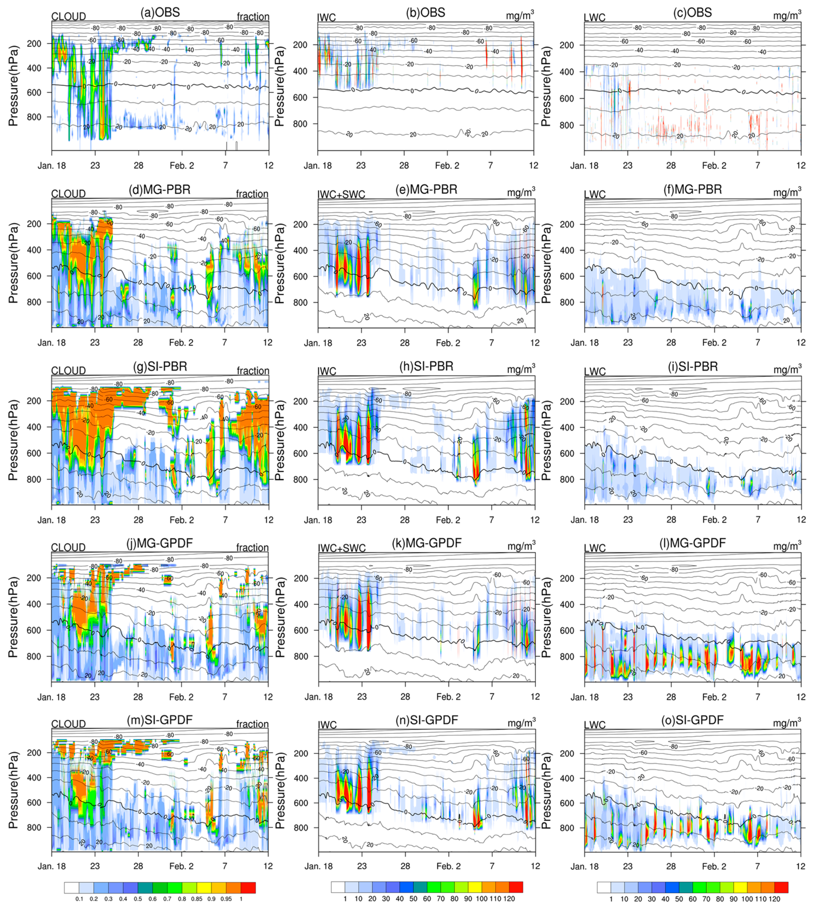
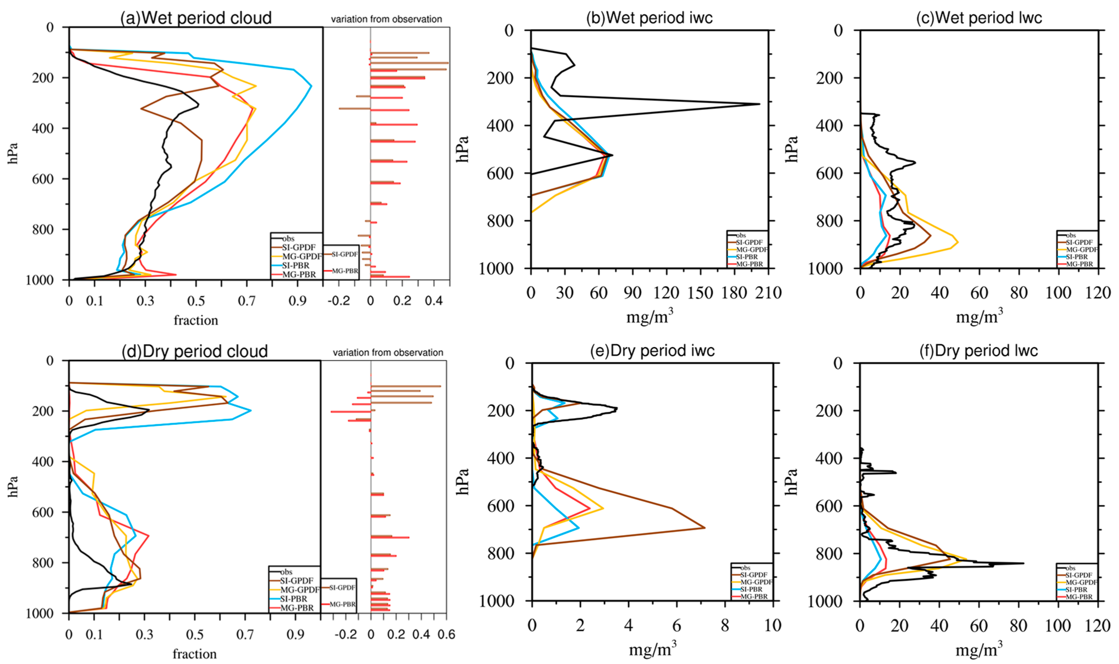
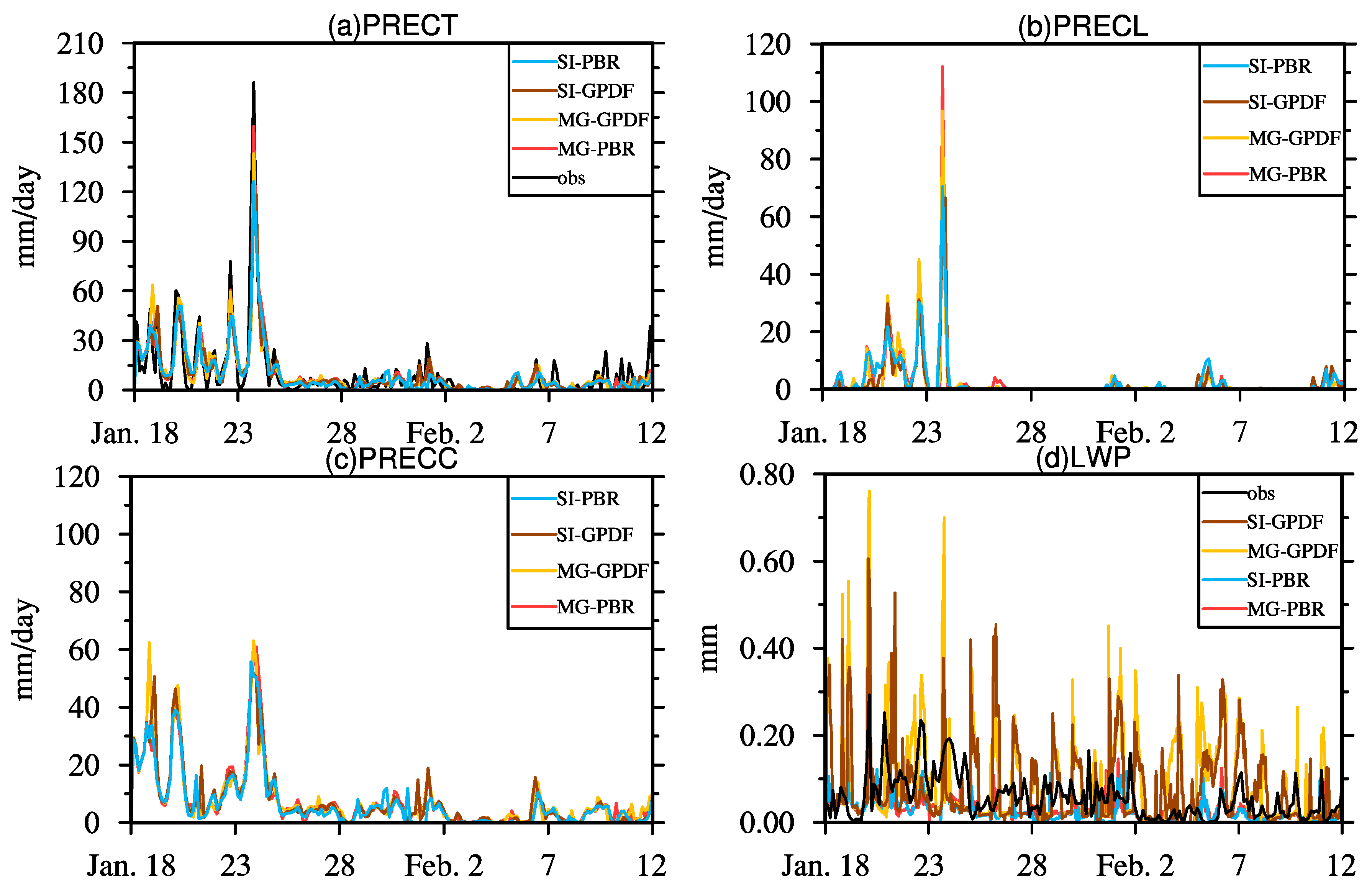
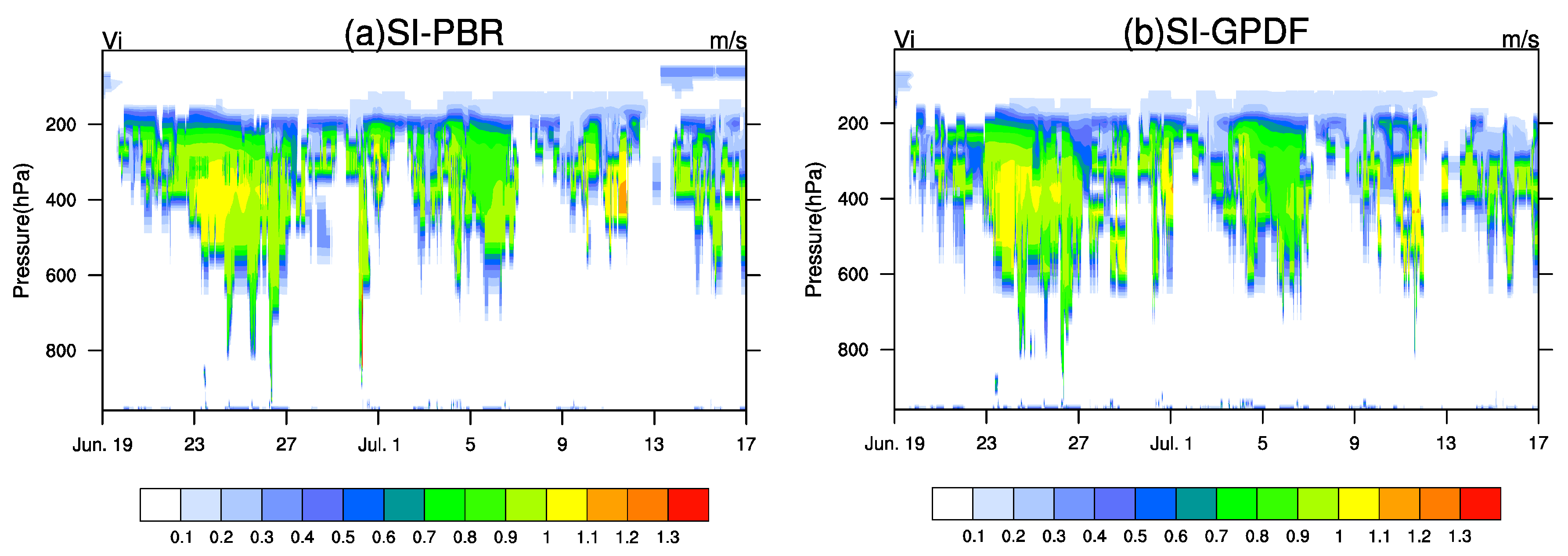
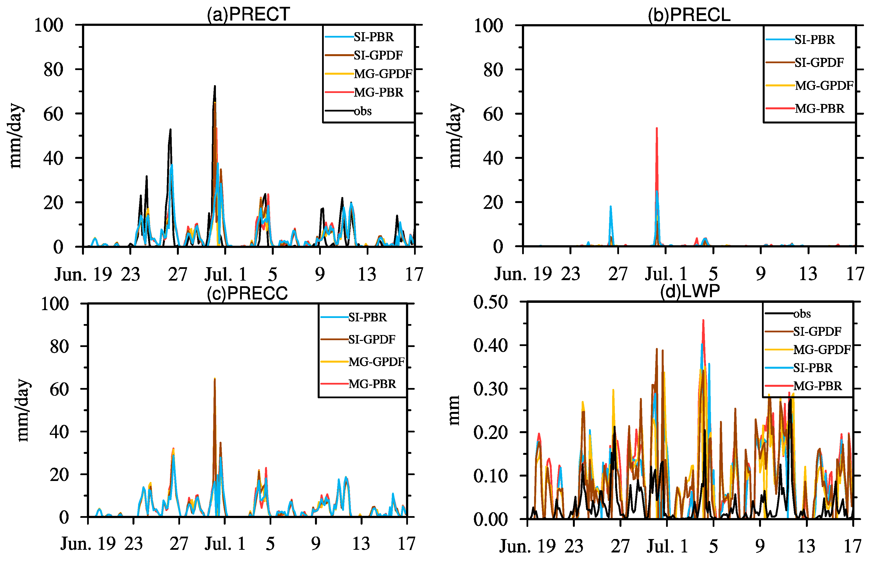
3.1. TWP-ICE Simulation

The TWP-ICE case was first simulated with the reference micro- (MG08) and macrophysics (PBR14) schemes in the MG-PBR run, and the updated schemes of SI and Gauss-PDF instead, respectively. Figure 1 shows the simulations of the cloud fraction, ice water content, liquid water content, and atmospheric temperature in comparison with the observations and retrievals in the IOP period. Without relaxed forcing in the SGRIST used here, the melting level varied obviously with time in this case simulation, even if the observation displayed a quasi-invariant height of the 0 °C isotherm. The substitution of the MG08 and PBR14 with the SI and Gauss-PDF, respectively, shows obvious difference of the cloud fraction, ice water and liquid water contents. When compared to the MG-PBR, the SI-PBR simulated a significant increase of clouds. In the monsoon active period, deep convection was active, and the cloud was observed in the troposphere (Figure 1g), especially above 700 hPa. The thickening of the cloud is well simulated during 18 and 25 January with the SI and PBR14 schemes with an overestimation of the cloudiness in the mid and upper troposphere in the convectively active period. In the convection-suppressing period, 26 January to 2 February, when the air was dry, cloudiness in the lower troposphere is associated with shallow convections and that at 200 hPa was displayed in the observations depicted in Figure 1a. The simulation of the high-level cloud amount was improved obviously with a cloud fraction of approximately unity by the SI scheme (Figure 1g), while the MG-PBR did not produce any cloudiness over 300 to 100 hPa in this dry period, which is quite different from the results in SCAM [16]. The ice water content also showed an increase in the simulation with the SI and PBR14 schemes (Figure 1h) in the wet convective phase before 25 January. The base of the ice water reaches 700 hPa in Figure 1h, which was much higher than the base height at 750 hPa below the melting level shown in Figure 1e. The observed melting level extended to 550 hPa without ice existing below the melting level (Figure 1b). The SI scheme ameliorated undershot of the ice water distribution under the melting level. In the convection suppressing period, the SI scheme also simulated a reasonable distribution of ice water content at 200 hPa, which was close to the observations. On 11 February, it is notable that extreme ice water content was display at 300 hPa, just as the observation. The updated SI scheme can improve the oceanic microphysics simulation, as indicated in this case study with the SGRIST model.
In the SI-GPDF test (Figure 1m–o), the cloud fraction, ice water, and liquid water contents simulated with the Gauss-PDF scheme instead of the PBR14 macrophysics are displayed. The cloud fraction was clearly improved below/above 200 hPa in the wet/dry period. The SI-GPDF successfully simulated the cloud fraction above 200 hPa during the dry period (Figure 1a), while the MG-PBR failed (Figure 1d). The statistical distribution of the subgrid moisture and temperature refined the diagnosis of the cloudiness and, therefore, ameliorates the vertical distribution of the cloud fraction in comparison with the observation (Figure 1a) and the numerical result with the referencing scheme (Figure 1d). The liquid cloud water was much more simulated below the melting level with the Gauss-PDF than that with the PBR14 in the numerical test. In the Gauss-PDF scheme, the subgrid variance of temperature and moisture are determined by shallow convection and boundary-layer turbulence, and the low-level condensation was therefore determined instantaneously as the cloudiness that showed clear increase in the lower troposphere (Figure 1c).
When the SI micro- and the Gauss-PDF macrophysics were both selected for the TWP-ICE simulation in the SI-GPDF test, temporal evolution of the vertical distribution of ice water and liquid water contents all showed notable ameliorations when compared to the reference simulation, even though the cloud fraction displayed further overestimation. The schemes caught the vertical cloudiness development, even if overestimation was found, mainly due to the ice cloud diagnosis. Thick cloud was simulated in the convectively active period (Figure 1m), and both thin lower and upper cloud layers were observed below 600 hPa and at 200 hPa, respectively. General cloudiness distribution showed agreement with the observation, especially when focusing on the upper-level (above 300 hPa) ice cloud after 25 January. The underestimate of the ice water content below the melting level was also improved in the wet phase, just as the SI scheme, and the ice water at 200 hPa was reasonably reproduced in the dry phase by the updated micro- and macrophysics. The liquid water content distribution was further enhanced, in which a thinner liquid water layer was simulated under the melting level in comparison with the MG-GPDF results.
We note that a sharp vertical variation of the cloud fraction, jumping from 50% to 95%, using the PBR14 scheme, was improved in the SI-GPDF simulation by updating the ice cloud diagnosis, as noted in Section 2. The vertical variation of the cloudiness is shown in Figure 1m.
Vertical profiles of cloud fraction, ice water, and liquid water contents averaged in the wet and dry periods are displayed in Figure 2. In the wet phase, vertical profile of cloud fraction displayed greater cloudiness in the mid-upper troposphere in the SI-PBR than the observations, due to the total ice being considered in the SI scheme (Figure 2a). The MG-GPDF and MG-PBR also showed an overestimation of cloudiness in the middle and upper levels. In SI-GPDF test, the cloud fraction was better simulated below 200 hPa, even though an overestimation was observed above. We calculated the statistical feature of the vertical profiles for quantitative description and easy understanding. In the SI-GPDF simulation, the root mean square error (RMSE) of the cloud fraction below 200 hPa was 0.1/0.08 in the wet/dry period, being smaller than 0.11/0.11 in the MG-PBR simulation. The simulated deviation of cloud fraction from the observations also illustrated a general amelioration with the SI-GPDF (Figure 2a,d). Besides the uncertainty of simple cloud diagnosis, a large error in the observational retrieval of cloud fraction is imaginable. Ice water content was well simulated below 500 hPa in both SI-PBR and SI-GPDF simulations with a total decrease of 21.57% below the melting level in comparison with that in the MG-PBR. The evidence can be found in Figure 2b that approximately the same ice water content is shown in the SI-PBR and SI-GPDF, but a large separation in the MG-PBR and MG-GPDF. However, the cloud water content was concentrated in lower levels with a significant difference among the four numerical experiments. The averaged profile of liquid water content was evidently improved below 700 hPa by the updated the SI and Gauss-PDF schemes in the SI-GPDF. The liquid water content in the SI-GPDF, approximately matched with the observation, was twice of that in the MG-PBR, which confirms the improved performance of the SI and Gauss-PDF schemes.
In the dry phase, either the SI or the Gauss-PDF can reproduce the cloudiness at 200 hPa in the SI-PBR, MG-GPDF, and SI-GPDF tests (Figure 2d), even though an over estimation is displayed. The large difference of cloud fraction between the MG-PBR and SI-PBR suggests the consistency of the Gauss-PDF scheme in reproducing the upper-level cloudiness. The schemes showed similar results in the mid- and lower troposphere below 400 hPa. The ice water content was simulated very little in the convection suppressing period, which is consistent with the observation (Figure 2e). The liquid water showed similar vertical profile in the SI-PBR and MG-PBR, SI-GPDF, and MG-GPDF. The Gauss-PDF scheme displayed a markable improvement to the liquid water profile in lower troposphere (Figure 2f), which demonstrated the significance of the Gauss-PDF scheme in the dry phase of this case simulation.
In the wet phase, when convection was active, the microphysics showed to be dominant in the simulation as illustrated above. Key microphysical processes in the SI and MG08 schemes were investigated. Figure 3 displays the sublimation, melting, deposition, and conversion of cloud ice to snow (only in MG08). Cloud ice and snow are considered as total ice in the MG08 scheme for fair comparison, because only the cloud ice is specified in the SI scheme. Because of the fast-falling speed of snow, ice-trapping was observed at 300 hPa (Figure 3a) in MG08. Instantaneous snow melt was supposed at 2 °C in MG08, and rapid snow melting into rain took place at 700 hPa. Weak sublimation showed double minus peaks at 300 and 600 hPa. The prognostic total ice in the SI scheme, however, extended to a lower level across the melting level. A strong sublimation of ice particles occurred at 700 hPa, which was consistent with that in the MG08, and relatively weak melting took place in a thick layer from 300 to 800 hPa (Figure 3b). The deposition of ice particles displayed a similar distribution as in the MG08.
Simulated precipitation is shown in Figure 4 with different couples of micro- and macrophysics. Under the strong modulation of the large-scale advection, all four experiments produced reasonable precipitation. The heavy rain period before 25 January and weak rain period after 26 January are clearly distinguished in Figure 4a. The peaks of precipitation were all weaker than the observational ones in the four experiments in the convectively active period. An investigation of the model large-scale and convective precipitation showed the underestimation of peak large-scale precipitation, which was mainly a result of the microphysics. The use of the Gauss-PDF macrophysics produced considerable liquid water (Figure 1l,o) benefitting from the Gaussian distribution of subgrid temperature and moisture, which was related to the strong rainfall, through interaction with the microphysics.
The simulated liquid water path can be also verified by comparing to the observations. The PBR14 scheme produced a slightly weaker liquid water path than the observed one in the MG-PBR and SI-PBR tests. The Gauss-PDF scheme simulated the quite thick liquid water path in comparison with the observation in the MG-GPDF and SI-GPDF tests because the cloud was determined using a Gaussian probability distribution function, which made vapor condensation and cloud fraction increase.

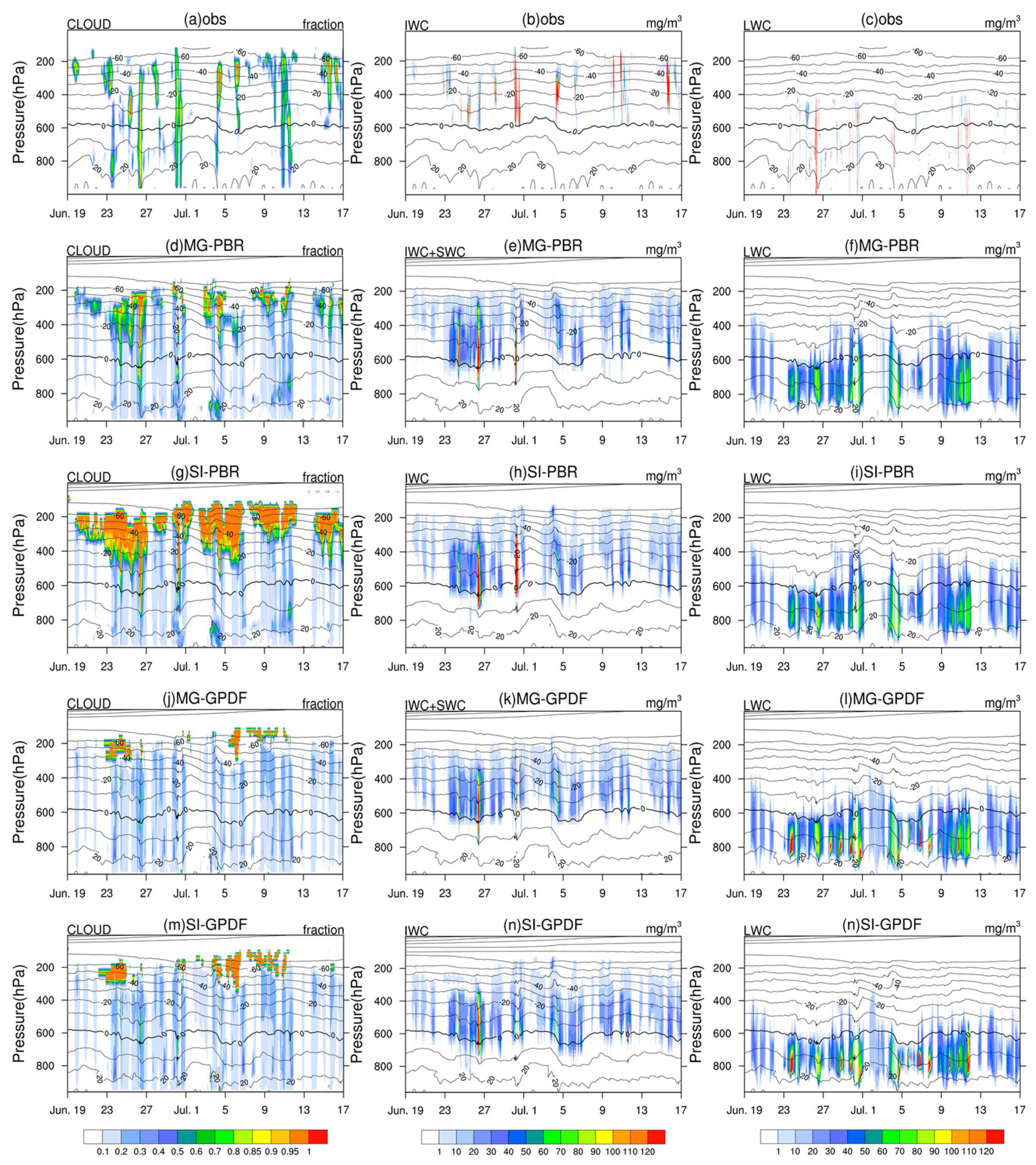
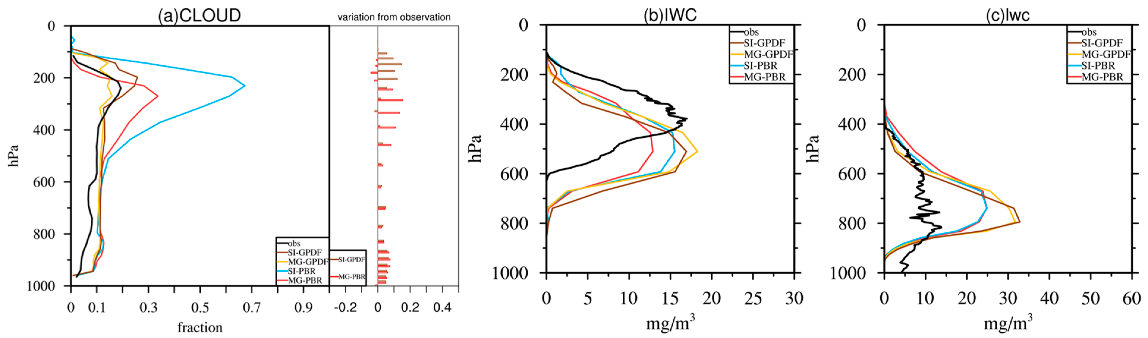
3.2. ARM97 Simulation

In addition to the evaluation of the micro- and macrophysics effects on oceanic surface, another IOP experiment, i.e., the ARM97, was used to verify the SI and Gauss-PDF schemes over land surface in more complex land-surface processes and planetary boundary-layer conditions. Figure 5 shows the simulated cloud fraction, ice water content, and liquid water content in numerical experiments of the MG-PBR, SI-PBR, MG-GPDF, and SI-GPDF, respectively, during the ARM97 IOP period. Regarding the cloud fraction, the MG08 scheme produced solid results in the MG-PBR and MG-GPDF, while the SI scheme simulated too much cloudiness above 400 hPa in the SI-PBR. The over estimation of the cloudiness, like the over prediction of ice at very high levels, was caused by the lack of ability to distinguish between cloud ice and snow. Relatively more cloud fraction was simulated above 200 hPa in the SI-GPDF than in the MG-PBR. However, below 200 hPa, the SI-GPDF displayed a good distribution of cloudiness in comparison with the observation (Figure 5a,d,m). The Gauss-PDF run displayed a little more cloud than the PBR14 run in the MG-GPDF and MG-PBR (Figure 5d,j), which tends to improve the simulation of cloud fraction, especially in lower levels (Figure 5a,d,j). The large peak values on 27 June in the SI-PBR and SI-GPDF were shown to be in agreement with the observation. Liquid water was simulated in lower levels in the four numerical tests, which was consistent with the observation. When compared with the results in the TWP-ICE simulations, liquid water was distributed in higher levels in ARM97. This may be related to the relatively large vertical gradient of temperature over land surface in summer, and the considerable vapor content in air over ocean. Water vapor and liquid water were easily transported to higher levels by thermal convections on land, despite the low melting level in ARM97 shown in both simulations and observations (Figure 5).
The vertical profiles of the cloud fraction, ice water, and liquid water contents averaged over the full period of simulations (Figure 6) display a similar feature as in the TWP-ICE (Figure 2). The SI scheme overestimated the upper-level cloudiness with the present method of ice cloud diagnosis. In the SI-GPDF, improved vertical distribution was displayed below 200 hPa with a similar peak level as the observation, even though the slightly overestimated cloud fraction could be found above. Smaller cloud fraction variance from the observation was shown below 200 hPa when compared to that in the MG-PBR. The RMSE of cloud fraction was 0.02 in the SI-GPDF and 0.04 in the MG-PBR. The overestimation of cloud fraction in upper troposphere may be partially due to the uncertainty of the tiny crystal observation with the satellite-based radar. Matched peak values of ice water content were illustrated in the four simulations, and the SI-GPDF contributed the best. All four experiments displayed lower vertical position of ice content as compared to the observation. The liquid cloud water showed its peak at 800 hPa using the Gauss-PDF scheme in both the SI-GPDF and MG-GPDF, while the peak appeared at 700~750 hPa in the SI-PBR and MG-PBR. The moisture PDF helped to improve the prognostic distribution of the liquid water content (Figure 6c) and liquid cloud (Figure 6a) in low levels. We must note that the uncertainty of retrieval of liquid water content is shown to be very large. The observational profile displayed here is the retrieval excluding the data that are greater than 0 but failed in minimum or maximum tests.
The temporal-vertical section of mass-weighted ice falling speed is given in Figure 7 to illustrate the reason of ice water existence below the melting level. The ice sedimentation speed reached 1.0 m/s at 400 hPa on 24 June in both numerical experiments (Figure 7). Ice water was observed below the melting level from 24 June to 26 June in the SI-PBR and SI-GPDF (Figure 5h,n) because of the falling speed of prognostic total ice reaching 0.8 m/s below 600 hPa (Figure 7a,b), which made the ice water drop below melting level. This suggests a way to further improve the SI scheme by tuning the melting rate and ice falling speed.
The precipitation and liquid water path in ARM97 simulations are also displayed in Figure 8. In general, precipitation was well produced in the four numerical simulations of the ARM97 case. The total precipitation depicted in Figure 8a also illustrated weaker peaks in this case, just as that in the TWP-ICE simulations. Out of the four couples of schemes, the pair of SI and Gauss-PDF simulated the largest peak of precipitation in the SI-GPDF test, which was the closest to the observation. The SI scheme, in cooperation with the PBR14 macrophysics scheme, produced the weakest large scale and convective precipitation (Figure 8b,c) under the interaction with other physical processes. The overestimated peak ice cloud water (Figure 5h) and underestimated liquid water (Figure 5i) on 27 June and 1 July resulted in insufficient grid-scale rainfall simulation, and possibly influenced the simulated intensity of convection and convective precipitation. In the SI-GPDF, a relatively weak peak of ice water (Figure 5n) and broad peak of liquid water (Figure 5o) were illustrated on 27 June and 1 July, which are related to the fine precipitation simulation.
In the four numerical experiments, liquid water path was simulated much more than the observation and it was not sensitive to the specific coupling of the micro- and macrophysics schemes. This was different from the illustration in the TWP-ICE simulations, which indicates the complexity of land–air interaction in the moist-process simulation because of the difficulty of land–surface characteristic specification.

4. Discussions and Conclusions

The SI microphysics was implemented into the SGRIST single-column model in cooperation with the Gauss-PDF macrophysics scheme because of the flexibility of the arrangement of total cloud ice and grid-scale dependent Gaussian PDF subgrid moisture distribution in the micro- and macrophysics schemes, respectively. The SI and Gauss-PDF schemes were evaluated with numerical simulation results of two cases, i.e., the TWP-ICE and ARM97, over ocean and land surfaces, respectively, and the IOP data. Four runs were conducted for each of the TWP-ICE and ARM97 cases with an arbitrary coupling of the microphysics schemes, the SI and MG08, and macrophysics schemes, the Gauss-PDF and PBR14, to show the numerical effect of precipitation simulation.
In a qualitative sense, the couple of the SI and Gauss-PDF show the proper vertical distribution of cloudiness in both the TWP-ICE and ARM97 simulations over ocean and land surfaces, respectively, even though an overestimation of the cloud fraction was still found in the upper troposphere. The vertical deviation and RMSE of cloudiness are obviously improved by the Gauss-PDF scheme, with the RMSE being reduced from 0.11/0.11 to 0.1/0.08 in wet/dry period of the TWP-ICE and 0.04 to 0.02 in the ARM97 case. The ice and liquid water contents were improved by the SI and Gauss-PDF schemes on either ocean or land surface, in better agreement with observations. The amount of ice cloud water and liquid water was more reasonably simulated with the SI and Gauss-PDF in comparison with the referencing schemes, especially the ice water dropping under the melting level. The use of the Gauss-PDF promoted the enhancement of liquid cloud water prediction in the microphysics, as shown in the MG-GPDF and SI-GPDF in both IOP experiments of the TWP-ICE and ARM97, which resulted in an overall increase of total precipitation peaks being consistent with the observations. The Gaussian distribution of subgrid temperature and moisture contributed to the water vapor assignment between large-scale and convective processes, which resulted in well simulated ice and liquid water contents and precipitation.
Moist process simulation is difficult because of the complexity of land–air interaction and land surface specification. The results in the ARM97 simulation showed differences from those in the TWP-ICE. The liquid water path was simulated very differently among the couples of schemes in the TWP-ICE, but it was similar in the ARM97. The overestimation of the cloudiness in upper levels was significant in the SGRIST with the new schemes. The diagnosis of cloud fraction can be tuned according to the results over different surfaces.

Author Contributions

Conceptualization, X.P. and Y.L.; Data curation, J.L.; Formal analysis, X.P. and J.L.; Funding acquisition, X.P. and Y.L.; Investigation, X.L., W.C. and J.L.; Methodology, X.P., X.L. and Y.L.; Project administration, X.P. and Y.L.; Supervision, X.P. and Y.L.; Validation, J.L. and X.P.; Visualization, J.L. and X.L.; Writing—original draft, J.L.; Writing—review & editing, X.P. and Y.L. All authors have read and agreed to the published version of the manuscript.

Funding

This research was funded by National key R&D program on monitoring, early warning, and prevention of major natural disasters (Nos. 2018YFC1507005 and 2018YFC1507001), National Natural Science Foundation of China (No. 42075151).

Institutional Review Board Statement

Not applicable.

Informed Consent Statement

Not applicable.

Data Availability Statement

The data in this study are available from the authors upon request ([email protected]).

Acknowledgments

Thanks two reviewers for their valuable comments.

Conflicts of Interest

The authors declare no conflict of interest.

References

  1. Tomita, H.; Goto, K.; Satoh, M. A new approach of atmospheric general circulation model: Global cloud resolving model NICAM and its computational performance. Siam J. Sci. Comput. 2008, 30, 2755–2776. [Google Scholar] [CrossRef]
  2. Zangl, G.; Reinert, D.; Ripodas, P.; Baldauf, M. The ICON (ICOsahedral Nonhydrostatic) modelling framework of DWD and MPI-M: Description of the non-hydrostatic dynamical core. Q. J. R. Meteorol. Soc. 2015, 141, 563–579. [Google Scholar] [CrossRef]
  3. Skamarock, W.C.; Klemp, J.B.; Duda, M.G.; Fowler, L.D.; Park, S.H.; Ringler, T.D. A multiscale nonhydrostatic atmospheric model using centroidal Voronoi tesselations and C-grid staggering. Mon. Weather Rev. 2012, 240, 3090–3105. [Google Scholar] [CrossRef] [Green Version]
  4. Weller, H.; Ringler, T.; Piggott, M.; Wood, N. Challenges facing adaptive mesh modeling of the atmosphere and ocean. Bull. Am. Meteorol. Soc. 2010, 91, 105–108. [Google Scholar] [CrossRef] [Green Version]
  5. Ringler, T.; Petersen, M.; Higdon, R.L.; Jacobsen, D.; Jones, P.W.; Maltrud, M. A multi-resolution approach to global ocean modeling. Ocean Model. 2013, 69, 211–232. [Google Scholar] [CrossRef]
  6. Harris, L.M.; Lin, S.-J.; Tu, C. High-resolution climate simulations using GFDL HIRAM with a stretched global grid. J. Clim. 2016, 29, 4293–4314. [Google Scholar] [CrossRef]
  7. Gettelman, A.; Callaghan, P.; Larson, V.E.; Zarzycki, C.M.; Bacmeister, J.T.; Lauritzen, P.H.; Bogenschutz, P.A.; Neale, R.B. Regional climate simulations with the community earth system model. J. Adv. Model. Earth Syst. 2018, 10, 1245–1265. [Google Scholar] [CrossRef] [Green Version]
  8. Zhang, Y.; Li, J.; Yu, R.C.; Zhang, S.; Liu, Z.; Huang, J.; Zhou, Y. A layer-averaged nonhydrostatic dynamical framework on an unstructured mesh for global and regional atmospheric modeling: Model description, baseline evaluation, and sensitivity exploration. J. Adv. Model. Earth Syst. 2019, 11, 1685–1714. [Google Scholar] [CrossRef] [Green Version]
  9. Bauer, P.; Thorpe, A.; Brunet, G. The quiet revolution of numerical weather prediction. Nature 2015, 525, 47–55. [Google Scholar] [CrossRef]
  10. Field, P.R.; Brozková, R.; Chen, M.; Dudhia, J.; Lac, C.; Hara, T.; Honnert, R.; Olson, J.; Siebesma, P.; de Roode, S.; et al. Exploring the convective grey zone with regional simulations of a cold air outbreak. Q. J. R. Meteorol. Soc. 2017, 143, 2537–2555. [Google Scholar] [CrossRef] [Green Version]
  11. Shin, H.H.; Hong, S.-Y. Representation of the subgridscale turbulent transport in convective boundary layers at gray-zone resolutions. Mon. Weather Rev. 2015, 143, 250–271. [Google Scholar] [CrossRef]
  12. Zhang, X.; Bao, J.W.; Chen, B.; Grell, E.D. A Three-Dimensional Scale-adaptive Turbulent Kinetic Energy Scheme in the ARW-WRF Model. Mon. Weather Rev. 2018, 146, 2023–2045. [Google Scholar] [CrossRef]
  13. Han, J.; Wang, W.; Kwon, Y.; Hong, S.-Y.; Tallapragada, A.; Yang, F. Updates in the NCEP GFS cumulus convection schemes with scale and aerosol awareness. Weather Forecast. 2017, 32, 2005–2017. [Google Scholar] [CrossRef]
  14. Jeworrek, J.; West, G.; Stull, R. Evaluation of cumulus and microphysics parameterizations in WRF across the convective gray zone. Weather Forecast. 2019, 34, 1097–1115. [Google Scholar] [CrossRef]
  15. Zhang, F.; Shen, Z.; Li, J.; Zhou, X.; Ma, L. Analytical delta-four-stream doubling-adding method for radiative transfer parameterizations. J. Atmos. Sci. 2013, 70, 794–808. [Google Scholar] [CrossRef]
  16. Zhao, X.; Lin, Y.; Peng, Y.; Wang, B.; Morrison, H.; Gettelman, A. A single ice approach using varying ice particle properties in global climate model microphysics. J. Adv. Model. Earth Syst. 2017, 9, 2138–2157. [Google Scholar] [CrossRef] [Green Version]
  17. Qin, Y.; Lin, Y.; Xu, S.; Ma, H.-Y.; Xie, S. A diagnostic pdf cloud scheme to improve subtropical low clouds in NCAR Community Atmosphere Model (CAM5). J. Adv. Model. Earth Syst. 2018, 10, 320–341. [Google Scholar] [CrossRef] [Green Version]
  18. Wicker, L.J.; Skamarock, W.C. Time-splitting methods for elastic models using forward time schemes. Mon. Weather Rev. 2002, 130, 2088–2097. [Google Scholar] [CrossRef]
  19. Li, X.; Zhang, Y.; Peng, X.; Li, J. Using a single column model (SGRIST1.0) for connecting model physics and dynamics in the Global-to-Regional Integrated forecast SysTem (GRIST-A20.8). Geosci. Model Dev. 2021. preprint for discussions. [Google Scholar]
  20. Neale, R.B.; Chen, C.; Lauritzen, P.H.; Williamson, D.L.; Conley, A.J.; Smith, A.K.; Mills, M.; Morrison, H. Description of the NCAR Community Atmosphere Model (CAM 5.0); NCAR Tech. Note 2012, NCAR/TN-4861 STR; National Center for Atmospheric Research: Boulder, CO, USA, 2012; Available online: http://www.cesm.ucar.edu/models/cesm1.0/cam/docs/description/cam5_desc.pdf (accessed on 19 December 2019).
  21. Zhang, G.J.; Mcfarlane, N.A. Sensitivity of climate simulations to the parameterization of cumulus convection in the Canadian Climate Centre general circulation model. Atmos. Ocean 1995, 33, 407–446. [Google Scholar] [CrossRef] [Green Version]
  22. Morrison, H.; Gettelman, A. A new two-moment bulk stratiform cloud microphysics scheme in the Community Atmosphere Model, version 3 (CAM3). Part I: Description and numerical tests. J. Clim. 2008, 21, 3642–3659. [Google Scholar] [CrossRef]
  23. Park, S.; Bretherton, C.S.; Rasch, P.J. Integrating cloud processes in the community atmosphere model, version 5. J. Clim. 2014, 27, 6821–6856. [Google Scholar] [CrossRef]
  24. Park, S.; Bretherton, C.S. The university of Washington shallow convection and moist turbulence schemes and their impact on climate simulations with the community atmosphere model. J. Clim. 2009, 22, 3449–3469. [Google Scholar] [CrossRef]
  25. Bretherton, C.S.; Park, S. A new moist turbulence parameterization in the community atmosphere model. J. Clim. 2009, 22, 3422–3448. [Google Scholar] [CrossRef]
  26. Iacono, M.J.; Delamere, J.S.; Mlawer, E.J.; Shephard, M.W.; Clough, S.A.; Collins, W.D. Radiative forcing by long-lived greenhouse gases: Calculations with the AER radiative transfer models. J. Geophys. Res. Atmos. 2008, 113, D13103. [Google Scholar] [CrossRef]
  27. Niu, G.-Y.; Yang, Z.L.; Mitchell, K.E.; Chen, F.; Ek, M.B.; Barlage, M.; Kumar, A.; Manning, K.; Niyogi, D.; Rosero, E.; et al. The community Noah land surface model with multiparameterization options (Noah-MP): 1. Model description and evaluation with local-scale measurements. J. Geophys. Res. Atmos. 2011, 116, D12109. [Google Scholar] [CrossRef] [Green Version]
  28. Lin, Y.; Colle, B.A. A new bulk microphysical scheme that includes riming intensity and temperature-dependent ice characteristics. Mon. Weather Rev. 2011, 139, 1013–1035. [Google Scholar] [CrossRef]
  29. Heymsfield, A.J.; Bansemer, A.; Twohy, C.H. Refinements to ice particle mass dimensional and terminal velocity relationships for ice clouds. Part I: Temperature dependence. J. Atmos. Sci. 2007, 64, 1047–1067. [Google Scholar] [CrossRef]
  30. Kim, S.Y.; Han, J.Y.; Choi, I.J.; Bae, S.Y. Evaluation of cloud and precipitation parameterization using a single-column model: A TWP-ICE case study. Asia-Pac. J. Atmos. Sci. 2014, 50, 469–480. [Google Scholar] [CrossRef]
  31. Cederwall, R.T.; Krueger, S.K.; Xie, S.; Yio, J. ARM/GCSS Single Column Model (SCM) Intercomparison, Procedures for Case 3: Summer1997 SCM IOP; Lawrence Livermore National Laboratory Rep. UCRL-ID-141823; Atmos. Sci. Div., Lawrence Livermore National Laboratory (LLNL): Livermore, CA, USA, 2000. [Google Scholar]
  32. Xie, S.; Hume, T.; Jakob, C.; Klein, S.A.; McCoy, R.B.; Zhan, M. Observed large-scale structures and diabatic heating and drying profiles during TWP-ICE. J. Clim. 2010, 23, 57–79. [Google Scholar] [CrossRef]
  33. Zhao, C.; Xie, S.; Klein, S.A.; Protat, A.; Shupe, A.D.; McFarlane, S.A.; Comstock, J.M.; Delanoë, J.; Deng, M.; Dunn, M.; et al. Toward understanding of differences in current cloud retrievals of ARM ground-based measurements. J. Geophys. Res. 2012, 117, D10206. [Google Scholar] [CrossRef]
Figure 1. Temporal-vertical plot of cloud fraction (left), ice water content (middle column) and liquid water content (right) in addition to the atmospheric temperature (solid, °C) in the MG-PBR (df), SI-PBR (gi), MG-GPDF (jl), and SI-GPDF (mo) simulation of the TWP-ICE in comparison with the observations and retrievals (ac). The melting level is marked with bold lines in the middle panels.
Atmosphere 12 00638 g001
Figure 2. Vertical profiles of cloud fraction and the deviation from the observation (a,d), ice water content (b,e) and liquid water content (c,f) averaged in the wet (18–25 January, top) and dry periods (26–30 January, bottom) in the four tests, MG-PBR (red), SI-PBR (cyan), MG-GPDF (orange), and SI-GPDF (brown) in comparison with the observations (black).
Atmosphere 12 00638 g002
Figure 3. Vertical profiles of microphysics processes for ice in the MG–PBR and SI–PBR experiments, sublimation (red), melting (cyan), deposition (orange), and auto-conversion of cloud ice to snow (brown), respectively, averaged in the wet period.
Atmosphere 12 00638 g003
Figure 4. (a) Total precipitation rate, (b) large-scale precipitation rate, (c) convective precipitation rate and (d) liquid cloud water path in the simulations MG-PBR (red), SI-PBR (cyan), MG-GPDF (orange), and SI-GPDF (brown) compared to the observation (black).
Atmosphere 12 00638 g004
Figure 5. Temporal-vertical plot of cloud fraction (left), ice water content (middle column) and liquid water content (right) in addition to the atmospheric temperature (solid, °C) in the MG-PBR (df), SI-PBR (gi), MG-GPDF (jl), and SI-GPDF (m,n,o) simulation of the ARM97 in comparison with the observations and retrievals (ac). The melting level is marked with bold lines in the middle panels.
Atmosphere 12 00638 g005
Figure 6. Vertical profiles of cloud fraction and the deviation from the observation (a), ice water content (b) and liquid water content (c) averaged during 19 June and 17 July in the four tests, MG-PBR (red), SI-PBR (cyan), MG-GPDF (orange), and SI-GPDF (brown) in comparison with the observations (black).
Atmosphere 12 00638 g006
Figure 7. Temporal-vertical plot of mass-weighted ice falling speed in (a) the SI-PBR and (b) the SI-GPDF.
Atmosphere 12 00638 g007
Figure 8. (a) Total precipitation rate, (b) large-scale precipitation rate, (c) convective precipitation rate and (d) liquid cloud water path in the simulations MG-PBR (red), SI-PBR (cyan), MG-GPDF (orange), and SI-GPDF (brown) compared to the observation (black).
Atmosphere 12 00638 g008
Table 1. Numerical experiments to evaluate the micro- and macrophysics schemes.
Exp. NameMG-PBRSI-PBRMG-GPDFSI-GPDF
MicrophysicsMG08SIMG08SI
MacrophysicsPBR14PBR14Gauss-PDFGauss-PDF
Publisher’s Note: MDPI stays neutral with regard to jurisdictional claims in published maps and institutional affiliations.

