
A Short-Term Wind Speed Forecasting Model Based on a Multi-Variable Long Short-Term Memory Network


1
School of Computer Science, Chengdu University of Information Technology, Chengdu 610225, China
2
Numerical Weather Prediction Center, CMA, Beijing 100081, China
3
School of Computer Science, University of Nottingham, Nottingham NG8 1BB, UK
*
Author to whom correspondence should be addressed.
Atmosphere 2021, 12(5), 651; https://0-doi-org.brum.beds.ac.uk/10.3390/atmos12050651
Submission received: 22 March 2021
/
Revised: 12 May 2021
/
Accepted: 16 May 2021
/
Published: 19 May 2021
(This article belongs to the Special Issue Recent Advances and Future Prospects of Machine Learning in Predictive Modeling of Atmospheric Sciences)
Abstract
:Accurately forecasting wind speed on a short-term scale has become essential in the field of wind power energy. In this paper, a multi-variable long short-term memory network model (MV-LSTM) based on Pearson correlation coefficient feature selection is proposed to predict the short-term wind speed. The proposed method utilizes multiple historical meteorological variables, such as wind speed, temperature, humidity, and air pressure, to predict the wind speed in the next hour. Hourly data collected from two ground observation stations in Yanqing and Zhaitang in Beijing were divided into training and test sets. The training sets were used to train the model, and the test sets were used to evaluate the model with the root-mean-square error (RMSE), mean absolute error (MAE), mean bias error (MBE), and mean absolute percentage error (MAPE) metrics. The proposed method is compared with two other forecasting methods (the autoregressive moving average model (ARMA) method and the single-variable long short-term memory network (LSTM) method, which inputs only historical wind speed data) based on the same dataset. The experimental results prove the feasibility of the MV-LSTM method for short-term wind speed forecasting and its superiority to the ARMA method and the single-variable LSTM method.
1. Introduction
Due to the shortage of conventional energy such as fossil fuels and increasingly severe environmental pollution, wind energy, as the most economical and environmentally friendly renewable energy, has attracted wide attention [1]. To improve the efficiency of wind energy utilization, it is important to achieve reliable and timely wind speed forecasting. However, it is a challenging task to establish a satisfactory wind speed prediction model because of the characteristics of wind speed, such as its intermittency, volatility, randomness, instability, and nonlinearity [2].
Wind speed forecasting can be classified according to the time scale, including very-short-term forecasting (minutes to one hour), short-term forecasting (on a time scale of hours to a day) [3], and long-term forecasting (on a time scale of months or years) [4]. Historically, short-term prediction was a concern only for the few grid utilities with high levels of wind power. More recently, however, due to the increase in the use of wind power in a greater number of countries, short-term wind forecasting has become a central tool for many transmission system operators (TSOs) or power traders in or near areas with considerable levels of wind power penetration [5]. To forecast short-term wind speed, researchers have developed several important prediction methods, which fall into four categories: (a) physical methods, (b) statistical methods, (c) machine learning methods, and (d) hybrid methods [6]. Hybrid approaches combine the first three learning methods to achieve better performance than that of a single method.
Physical methods often require comprehensive consideration of physical information, such as temperature, humidity, atmospheric pressure, topographic features of wind farms, and surface roughness, in order to establish an accurate geophysical model. The numerical forecast model, for example, must solve the equations of flow and thermodynamics that describe the evolution of the weather by using a high-performance computer. To predict the atmospheric motion state and weather conditions for a specific future period, it sets initial and boundary value conditions that reflect the actual conditions in the atmosphere [7]. The method is highly sensitive to initial error; thus, inaccurate initial values lead to a poor forecast performance. In addition, problems exist in the coordination of atmospheric numerical models, including the coordination between the vertical and horizontal resolutions of the models, and in the coordination between physical processes [8]. Due to the time scale, physical resolution, initialization times of the data, and the wind evolution, physical methods perform poorly in short-term wind speed prediction.
Statistical methods are also used for short-term wind speed forecasting; they include the autoregressive (AR) model, autoregressive moving average (ARMA) model, autoregressive integrated moving average (ARIMA) model, and filtering model [9]. These methods have been widely used in wind speed time-series prediction based on a large amount of historical data. Poggi et al. [10] employed the AR model for the prediction of wind speed at three Mediterranean sites in Corsica and demonstrated that the AR model can reproduce the mean statistical characteristics of the observed wind speed data. Kavasseri et al. [11] adopted the fractional ARIMA model to predict wind speed in North Dakota on the day-ahead and two-day-ahead horizons and highlighted that the developed model outperformed the persistence model. Lydia et al. [12] developed a linear model based on the Gauss–Newton algorithm and a non-linear AR model based on a data-mining algorithm to forecast ten-minute- and one-hour-ahead wind speed. However, as noted in [13], because the time-series model assumes that the wind speed time series is linear, whereas the actual wind speed is usually nonlinear, most statistical methods cannot effectively represent the wind speed time series with nonlinear characteristics. During wind power ramp events, in particular, statistical methods perform poorly.
Some recent studies have shown that the use of wind lidar measurements outperforms statistical models for very short-term wind speed forecasting. Long-range wind lidar is used to measure wind speed at multiple range gates along a laser beam, thus achieving very high temporal and spatial resolution, and achieving more accurate predictions of wind-ramping events by capturing small fluctuations in wind speed [14]. Valldecabres et al. used lidar measurements to predict near-coastal wind speed with lead times of five minutes [15]. Using Taylor’s frozen turbulence hypothesis with local terrain corrections, they demonstrated that wind speeds at downstream locations could be predicted using scanning lidar measurements taken upstream in very short periods of time [15]. This method has a higher prediction accuracy than those of the persistence method and the ARIMA model [15].
In recent years, with the development and evolution of computers, various machine learning methods have gradually been applied to time-series prediction, which include back-propagation (BP) neural networks [16], Bayesian networks (BNs) [17], wavelet neural networks [18], extreme learning machines (ELMs) [19], and recurrent neural networks (RNNs) [20]. Chen et al. [21] used multiple linear regression analysis, gray prediction, BP neural network prediction, a combined gray BP neural network prediction method, and long-term and short-term memory network model prediction methods to predict the energy consumption situation in Beijing, which provided a reference for the application of machine learning methods in time-series prediction. Zhou et al. [22] used a back-propagation (BP) neural network with ship navigation behavior data as the training data to predict a ship’s future navigation trajectory. Based on information from the Automatic Identification System (AIS) on the waters near the Nanpu Bridge in Pudong New Area, Shanghai, the experimental results showed that, compared with the traditional method of kinematic trajectories, the model can be more effective for predicting ship navigation. Guo et al. [23] developed four wavelet neural network models using the Morlet function as the wavelet basis function to forecast short-term wind speed in the Dabancheng area in January, April, July, and October. It was shown that the prediction accuracy of the model, which has more neurons in the hidden layer than other models, satisfied industrial wind power forecasting requirements. ELMs have received extensive attention in recent years due to their characteristics such as fast predictive speed, simple structure, and good generalization [24]. Zhang et al. [19] developed a combination model based on ELMs for wind speed prediction in Inner Mongolia, and its main technologies included feature selection and hybrid backtracking search optimization tools. The RNN method has the characteristics of sharing memory and parameters, so it has certain advantages in learning the nonlinear characteristics of sequences. Therefore, in recent years, there have been many studies of the application of RNNs for time-series prediction. Fang et al. [25] used long short-term memory network (LSTM) and deep convolution generative adversarial networks (DCGANs) to construct a prediction model for sequential radar image data, and compared it with 3DCNN and CONVLSTM; the proposed method was more robust and effective, and is theoretically applicable to all sequence images. Yan et al. [26] used a long short-term memory network (LSTM) to predict the increase in the number of new coronavirus disease infections. The experimental results showed that the LSTM had higher prediction accuracy than the traditional mathematical differential equation and population prediction model. Liu et al. [27] designed two types of LSMT-based architectures for prediction of one-step and multi-step wind speed to alleviate the influence of its nonlinear and non-stationary nature. Chen et al. [28] used LSTM as a predictor to develop the EnsemLSTM method using an ensemble of six single, diverse methods for ten-minute- and one-hour-ahead wind speed forecasting. Hu et al. [2] introduced a differential evolution (DE) algorithm to optimize the number of hidden layers in each LSTM and the neuron count in each hidden layer of the LSTM for the trade-off between learning performance and model complexity. These examples show that the LSTM has more advantages in short-term wind speed prediction than traditional machine learning algorithms. The LSTM performs well in time-series prediction, so LSTM networks can be regarded as powerful tools for wind speed prediction.
Based on the above analysis, considering that changes in wind speed will be greatly affected by other weather factors, a multi-variable LSTM network based on Pearson correlation coefficient feature selection is proposed in this paper (MV-LSTM). The proposed model is trained on historical data for wind speed, temperature, humidity, air pressure, and other meteorological elements to predict the short-term wind speed at Yanqing and Zhaitang sites in Beijing, China. Section 2 of this paper describes the experimental data, the theoretical background of the proposed method, and how it is implemented. Section 3 shows the results of the experiments and analyzes them with the evaluation metrics. Section 4 summarizes the performance of the proposed method on the dataset and proposes possible measures for improving the model.
2. Data and Methods
2.1. Site Description
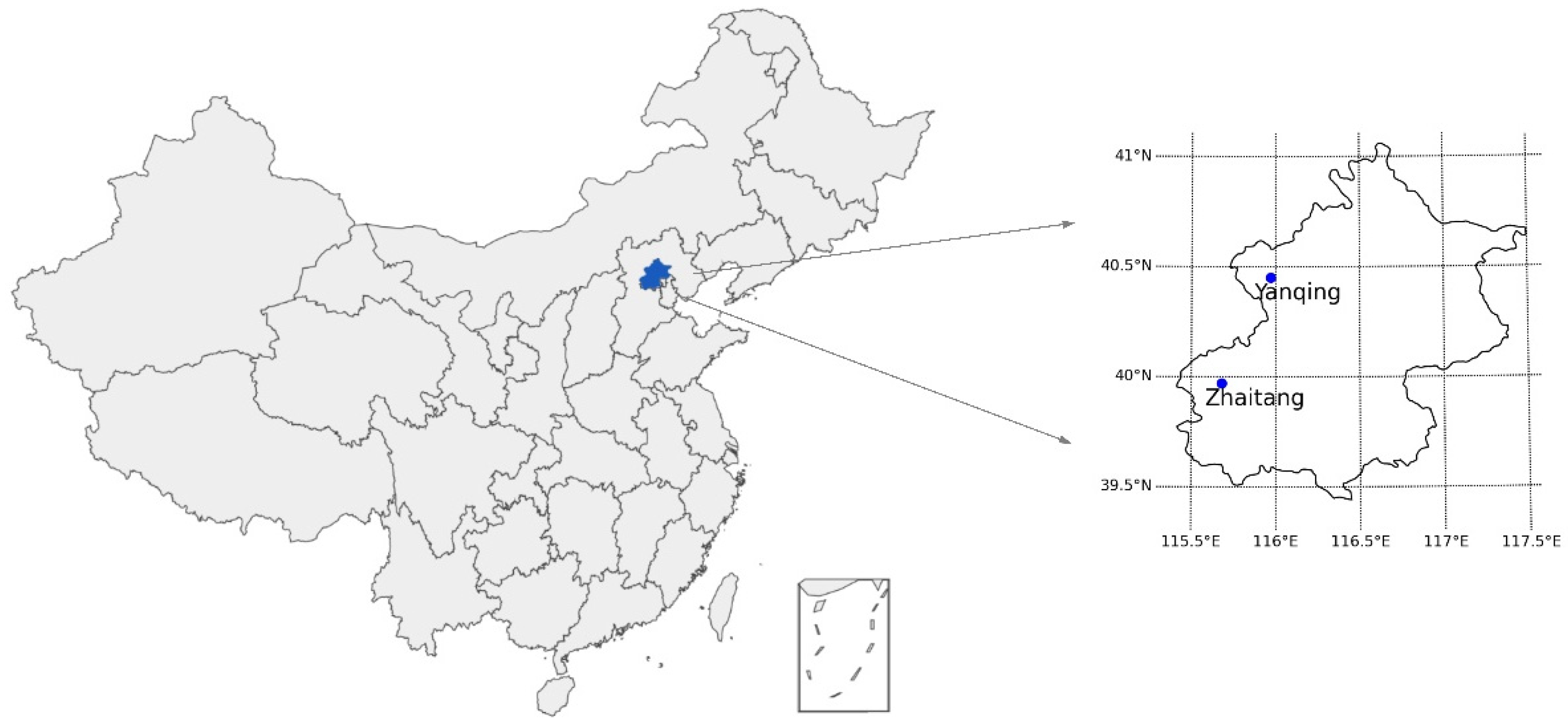
In this study, the data used in the experiments were taken from two sites—Yanqing and Zhaitang in Beijing, Northeast China—which experience a temperate continental monsoon climate. Yanqing station is located in Yanqing County, Beijing. The Yanqing Badaling Great Wall Basin is surrounded by mountains on three sides in the north and southeast, and by the Guanting Reservoir to the west—namely, the Yanhuai Basin. Yanqing is located in the east of the basin, with an average elevation of about 500 m. The area is dominated by southwestern winds in winter and southeastern winds in summer, with an average annual wind speed of 3.4 m/s at a height of 10 m above the ground, and the wind resources account for 70% of Beijing’s wind resources. Zhaitang station is located in Zhaitang Town, Beijing. Zhaitang Town is located in the middle of the Mentougou mountainous area and belongs to a warm temperate zone with a semi-humid and semi-arid monsoon climate. The area is dry and windy in spring, which has the highest wind speed throughout the year, followed by that of the winter. The locations of the stations shown in Figure 1. Table 1 presents the geographical coordinates of the two stations.
2.2. Data Description
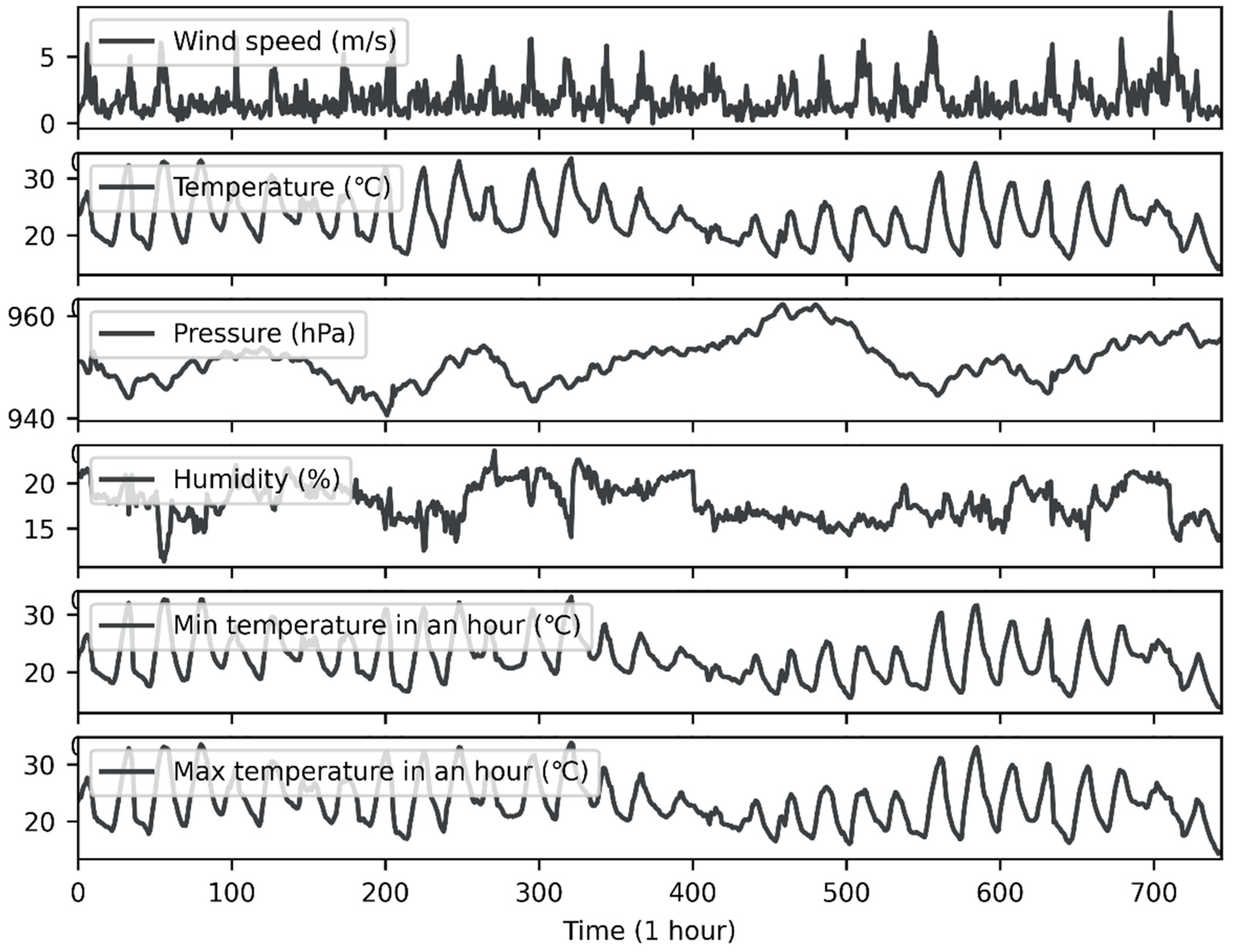
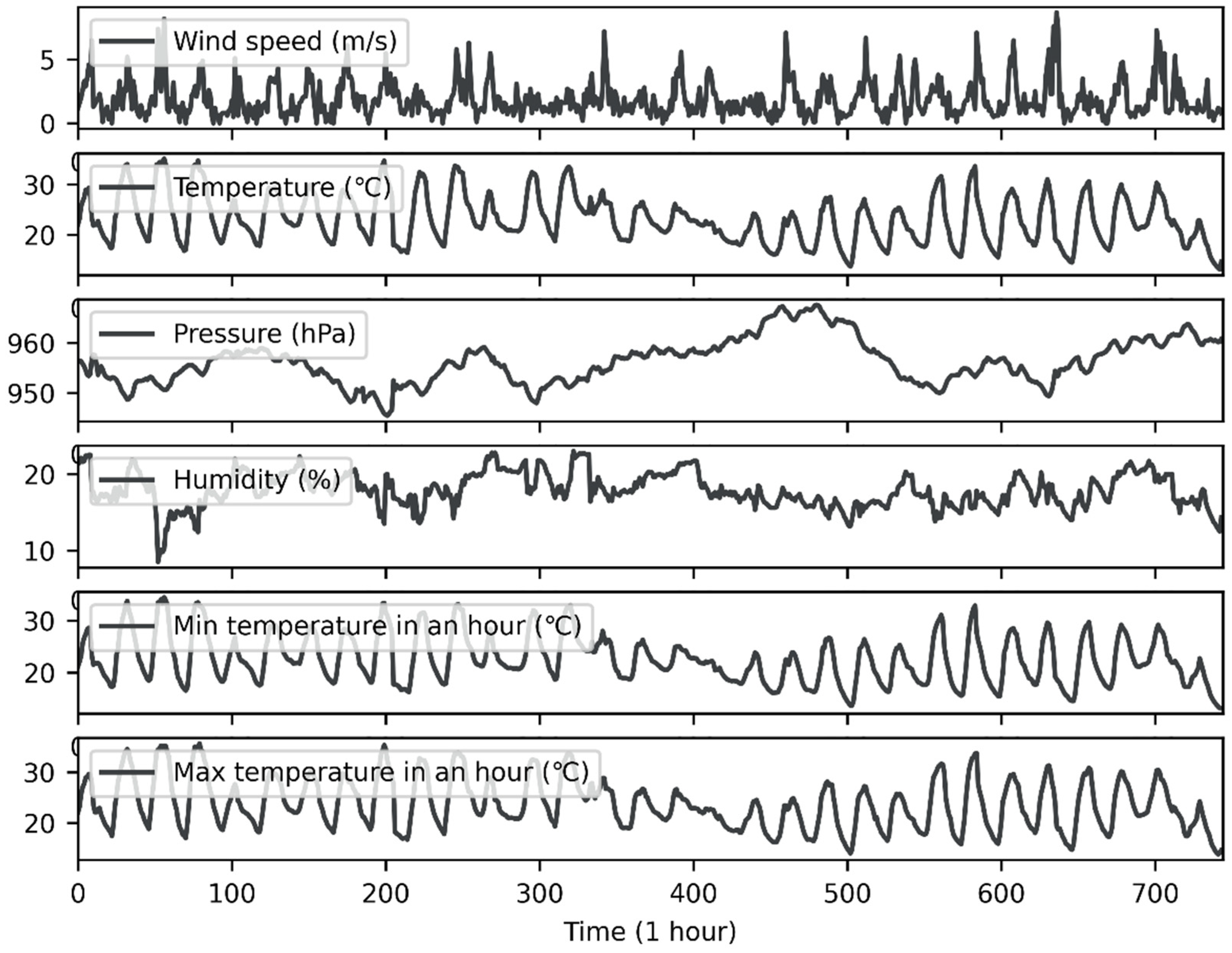
The experimental data were hourly observation data from ground observation stations (Yanqing and Zhaitang stations) provided by the China Meteorological Administration from 1 August 2020, to 31 August 2020. Figure 2 and Figure 3 show time-series diagrams of observations from the two stations. As the figures show, the data for each site included 744 samples (31 days × 24 h). In addition to the wind speed (m/s), which was measured at a height of 10 m above the ground, the meteorological elements at each point in time included surface temperature (°C), surface pressure (hPa), relative humidity (%), one-hour precipitation (Rain1h) (mm), one-hour maximum temperature (MaxT) (°C), and one-hour minimum temperature (MinT) (°C).
In this study, the time-series data for all meteorological elements were used to predict short-term wind speed one hour in advance. For each station, hourly observations between 1 August 2020 and 25 August 2020 (the top 80% of the total data; 25 days × 24 h = 600 samples of data) were used to train the model, and hourly observations between 26 August 2020 and 31 August 2020 (the bottom 20% of the total data; 6 days × 24 h = 144 samples of data) were used to test the model. To address the issue of missing values, we used the mean value of the two data points before and after the missing data point as a proxy.
2.3. Prediction Methods
To scientifically evaluate the performance of the proposed model, we selected a classical time-series model, the ARMA model (a random series model that is trained with past data to predict future data), for a control experiment. (Readers can obtain more information about ARMA by referring to [29].)
The following is an introduction to the LSTM model.
2.3.1. Long Short-Term Memory (LSTM) Networks
An LSTM network is a special recurrent neural network (RNN). Therefore, before introducing LSTM, we provide a brief introduction to RNNs. We introduce the advantages of RNNs compared to traditional neural networks in processing time-series data, and their shortcomings in respect of long-term memory (an LSTM network was proposed to solve this problem).
Recurrent Neural Networks (RNNs)
A traditional neural network is fully connected from the input layer to the hidden layers and then to the output layer; however, the neurons between each layer are not connected, which leads to large deviations in the results of traditional neural networks when processing sequence data [30]. Unlike traditional neural networks, recurrent neural networks (RNNs) can remember the previous information and apply it to the current output calculation; that is, the neurons between the hidden layers are connected, and the input of the hidden layer is composed of the output of the input layer and the output of the hidden layer at the previous moment.
Based on the characteristics of sequential data processing, a common RNN training method is the back-propagation through time (BPTT) algorithm. This algorithm is characterized by finding better points along the negative gradient direction of parameter optimization until convergence. However, in the optimization process, to solve the partial derivative of parameters at a certain moment, the information for all moments before that moment should be traced back, and the overall partial derivative function is the sum of all moments. When activation functions are added, the partial multiplications will result in multiplications of the derivatives of the activation functions, which will lead to “gradient disappearance” or “gradient explosion” [31].
Long Short-Term Memory (LSTM) Networks
To solve the problem of gradient disappearance or gradient explosion in RNNs, Horchreiter et al. [32] proposed LSTM in 1997, which combines short-term and long-term memory through gate control, thus solving the above problems to a certain extent.
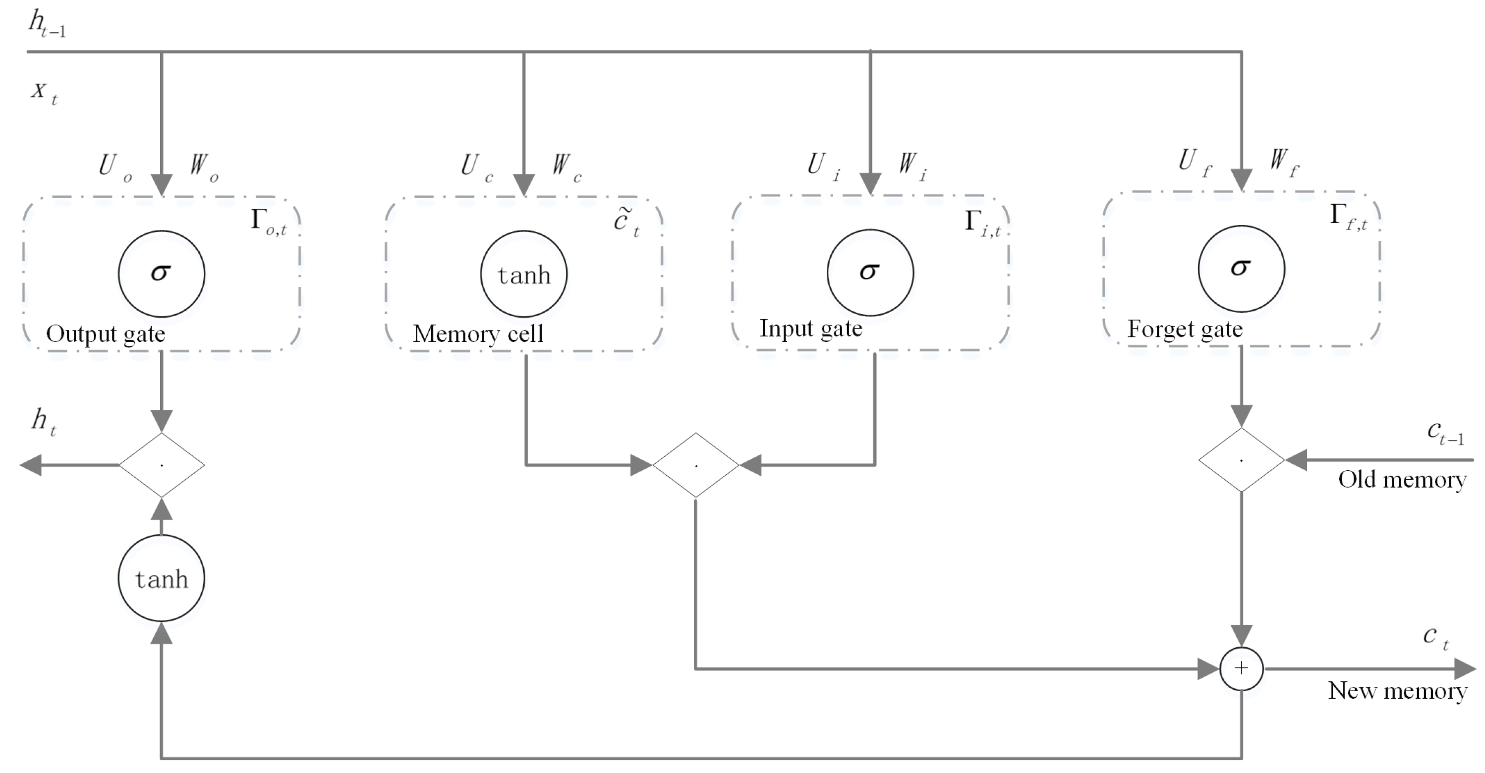
Figure 4 shows the basic structure of an LSTM cell. It has an input gate Γi an output gate Γo, a forgetting gate Γf, and a memory cell . ht is the hidden state at time point t, xt is the input of the network at time point t, and σ is the activation function (sigmoid).V, W, and U are the neurons’ shared weight coefficient matrix.
An LSTM network protects and controls information through three “gates”:
- 1.
- The forgetting gate determines what information in needs to be discarded or retained. By obtaining and , the output [0, 1] is assigned to , where 1 means completely retained and 0 means completely discarded. The output of the forgetting gate is as follows (where is the bias vector of the hidden layer element, is the bias vector, and the subscript is the corresponding element):
- 2.
- The input gate determines how much information to add to the cell and generates the information of the sigmoid and tanh by combining with the forgetting gate to update the state of the cell. The input gate steps are:
- 3.
- The output gate determines which part of the information of the current cell state is used as the output, and is still completed by the sigmoid and tanh. The output gate steps are:
According to the above steps, the LSTM model can deal with long-term and short-term time-dependent problems well.
The steps of the LSTM model method are as follows:
Step (1): Data normalization
As stated in Section 2.1, we used the first 80% of data in the time series of observation data for the training model and the last 20% of the data for the testing model. Table 2 shows the statistics for the training set and the test set.
To ensure the input wind observations shared the same structures and time scales [33], we used the maximum and minimum values in the training set to normalize the input of the model (scaling the data to 0–1), and we reverse normalized the output data (scaled the data from 0–1 back to normal data). The normalized data were computed with:
where is the normalized feature value for time . is the maximum value of the training dataset for one feature. is the real value at time . is the minimum value of the training data for one feature. The wind speed, temperature, pressure, humidity, minimum temperature, and maximum temperature were all normalized to 0–1 with the above equation.
Step (2): Data formatting
We used Keras, a third-party Python library, to set up the LSTM network. LSTM is a supervised learning model (supervised learning means that the training data used to train the model needed to contain two parts: the sample data and the corresponding labels). The LSTM model in Keras assumes that the data are divided into two parts: input X and output Y, where input X represents the sample data and Y represents the label corresponding to the sample data. For the time-series problem, the input X represents the observed data for the last several time points, and the output Y represents the predicted value of the next time point (this can be understood as follows: we input the wind speed observation values from the last several hours into the model, and the model outputs the wind speed for the next hour). Therefore, both the training and test sets need to be formatted in two parts: X and Y. Equations (7) and (8) represent the data format:
where is the time step. We set this to 8, which means that the last 8 h of wind speed observations are used to predict the next hour’s wind speed. indicates sample , indicates the label corresponding to sample and is the wind speed at time .
For the training set, according to Equation (7), 592 (n = total data size − time steps = 600 − 8 = 592) samples were input into the LSTM network, and each sample contained wind speed observation values for 8 h. According to Equation (8), the labels corresponding to the samples contain the wind speed observation values from the 9th hour to the 600th hour. For example, the first sample contains the wind speed observation values for 8 h from the first hour to the eighth hour, and its corresponding label is the wind speed observation value of the ninth hour. The sample data and corresponding labels were used together to train the model.
The test set was also labeled in the same way.
Step (3): Model training
We used the formatted training set data to train the LSTM network model. By iteratively learning the training data, the weight parameters of the network were optimized so that the model could learn the time-series characteristics of the wind speed. Table 3 shows the hyper-parameters of the LSTM network model. (We recommend that the reader obtains the specific meaning of each hyper-parameter from [34].)
According to Table 3, we divided the samples of the training set into 148 (=592/4) batches. All the batches were transmitted forward and back in the neural network for 30 epochs to train the model. In each epoch, we used MSE (the calculation is shown in Equation (9); is the prediction of wind speed at time , and is the observation of the wind speed at time ) to calculate the difference between the forward calculation result of each iteration of the neural network and the true value, and used ADAM to change each weight of parameters in the network so that the loss function was constantly reduced and the accuracy of the neural network was increased.
Step (4): Predicting the wind speed with the trained LSTM network model
The input of the model was X of the test set, which was obtained in step (2). The output of the model is shown in Equation (10):
where (or ) is the prediction of the wind speed at time .
It should be noted that the prediction is scaled in the range of 0–1, so it must be inversely normalized to obtain the wind speed prediction within the real range. Equation (11) describes how to inversely normalize the model output:
where is the wind speed prediction (within the real range) at time , is the maximum wind speed observation in the training set, and is the minimum wind speed observation in the training set. The reason for using the maximum and minimum values of the training set instead of the test set for inverse normalization is that in actual situations, we can only know the observed values of the wind speed in the past, so we can only use the past maximum and minimum wind speeds to predict the maximum and minimum wind speeds in the future.
2.3.2. Multi-Variable Long Short-Term Memory (MV-LSTM) Network
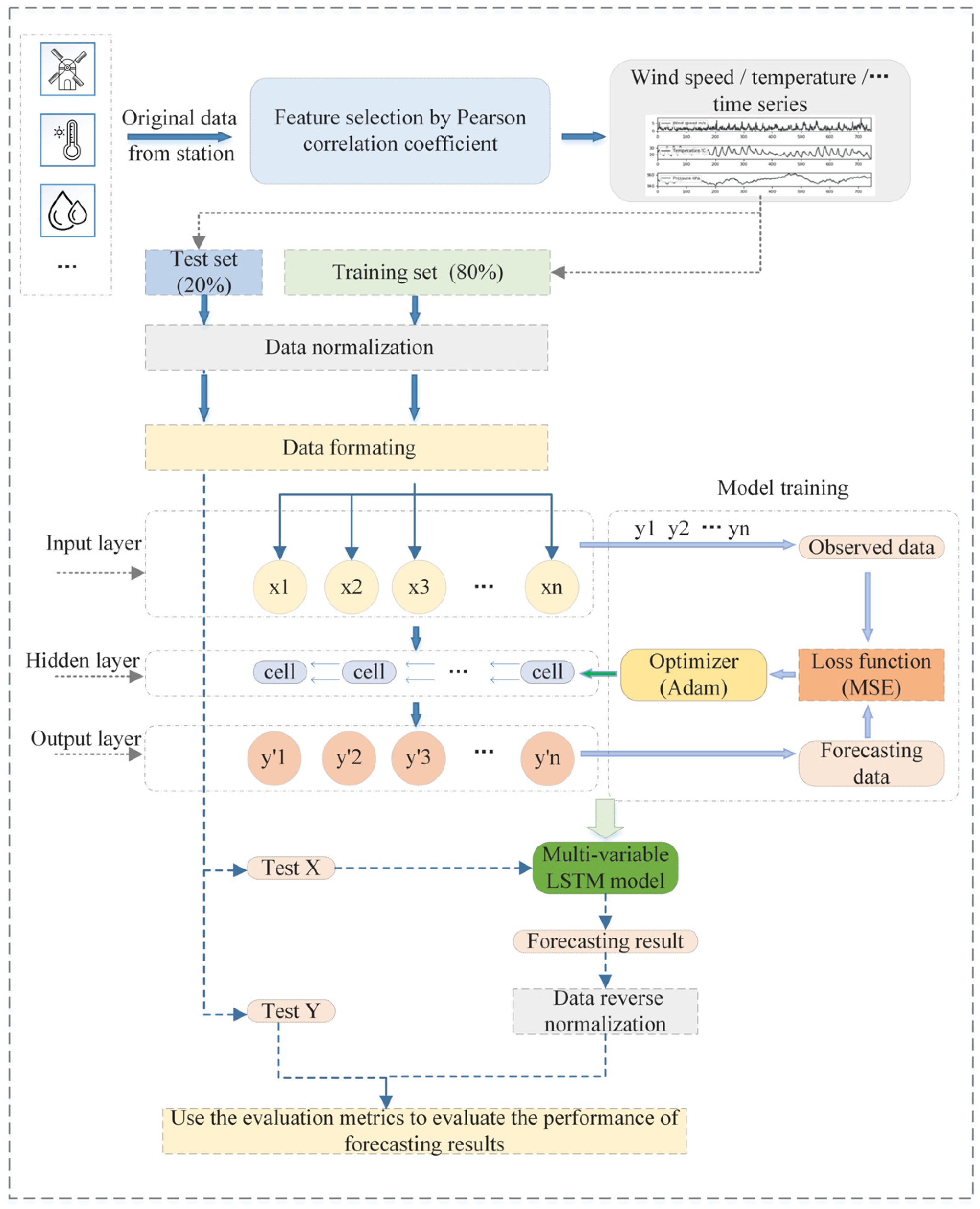
In this paper, we propose a multi-variable LSTM network model based on Pearson correlation coefficient feature selection for short-term wind speed prediction, which takes the historical data for multiple meteorological elements into account. The framework is shown in Figure 5.
The steps of the MV-LSTM network method are as follows:
Step (1): Feature selection
There is a certain correlation between different meteorological variables [35]. Therefore, we calculated the Pearson correlation coefficient between each meteorological element and the wind speed, identified several meteorological elements (features) that are significantly related to the wind speed, and used them in conjunction with the wind speed time series as the input of the model. Equation (12) describes how to calculate the Pearson correlation coefficient [36]:
where is the Pearson correlation coefficient between x and y, is the covariance between X and Y, is the standard deviation of X, and is the standard deviation of Y.
The Pearson correlation coefficient ranges from –1 to 1. When the correlation coefficient approaches 1, the two variables are positively correlated. When the correlation coefficient tends to –1, the two variables are negatively correlated [37]. The bigger the absolute value of the correlation coefficient, the stronger the correlation between the variables. However, it is not sufficient to discuss only the absolute value of the coefficient. Therefore, hypothesis testing was used in this study to discuss the correlation between each meteorological element and the wind speed:
- (1)
- We first propose the null hypothesis and the alternative hypothesis:The null hypothesis: which means that the two variables (X and Y) are linearly independent;The alternative hypothesis: , which means that the two variables are linearly dependent.
- (2)
- We calculate the probability value (p-value) of the null hypothesis being true (when the two variables are linearly independent).
- (3)
- We set the significance level: .
- (4)
- We compare the p-value to . If the p-value is less than , the null hypothesis is considered as the extreme case, thus rejecting the null hypothesis and accepting the alternative hypothesis, which means that the linear correlation between X and Y is statistically significant.
Table 4 lists the correlation between each meteorological element and the wind speed from the datasets for Yanqing Station and Zhaitang Station.
As can be seen in Table 4, when the significance level is set to 0.05, for the different stations, the meteorological elements related to wind speed were also different. Therefore, we built MV-LSTM models for Yanqing Station and Zhaitang Station separately. Both models used the same hyper-parameters (see Step (4) for details). The models for each station were trained and tested using observations from that station. In Yanqing Station, the meteorological elements, including the temperature, pressure, humidity, minimum temperature in 1 h, and maximum temperature in 1 h, were related to wind speed. Therefore, these meteorological variables and wind speed data were selected as the inputs of the MV-LSTM model for Yanqing Station. In Zhaitang Station, the meteorological elements, including the temperature, pressure, minimum temperature in 1 h, and maximum temperature in 1 h, were related to wind speed. Therefore, these meteorological variables and wind speed data were selected as the inputs of the MV-LSTM model for Zhaitang.
Step (2): Data normalization
Similarly to the single-variable LSTM method, to ensure the input meteorological variables share the same structures and time scales, the selected meteorological elements and wind speed sequences must be normalized. Step (1) in Section 2.3.2 describes how the wind speed sequence was normalized. For the MV-LSTM model, not only the wind speed, but also the meteorological elements selected by features, should be normalized. As an example, Equation (13) shows normalization of temperature:
where is the normalized temerature at time , is the temperature observation at time , is the minimum temperature of the training set, and is the maximum temperature of the training set. The segmentation method for the training set and test set was the same as that of the single-variable LSTM method (the first 80% of the data of each site were used as the training set, and the last 20% were used as the test set.).
Step (3): Data formatting
Similarly to the single-variable LSTM method, the datasets need to be transformed into a format for supervised learning. However, there is a difference between the single-variable LSTM method and MV-LSTM method for . Unlike in the single-variable LSTM method, which contains 8 h of wind speed observations (from the time i to the time i+7), in MV-LSTM contains 8 h of observations of several meteorological elements (including the wind speed and other meteorological elements selected as features). Equation (14) describes the data format of in MV-LSTM:
where is sample , and is the observations of the meteorological elements at time i. For Yanqing Station, , where , , , and are the temperature observation, the pressure observation, the humidity observation, the minimum temperature in the last hour at time and the maximum temperature in the last hour at time , respectively. For Zhaitang Station, .
Step (4): Model training
From step (3), for the training set and test set of each station, we obtained the corresponding and . We used and of each station’s training set to train the model for that station.
The hyper-parameters of the MV-LSTM network model are the same as that of the LSTM network.
in the training set enters the hidden layer through the input layer of the model, which has several cells. The meteorological element data for each moment () propagate among the cells, and the data for the past moment affect the output of the cell at the next moment through the gate control mechanism. When all samples in have propagated an epoch in the hidden layer, the model will output the predicted value of this epoch through the output layer. The difference between the predicted value and the observed value is calculated with the loss function. Then, the optimizer is used to make the model update the connection weight of each neuron in the hidden layer in the direction of the decreasing value of the loss function.
After 30 epochs, the trained MV-LSTM network model was obtained.
Step (5): Predicting the wind speed with the trained MV-LSTM network model
in the test set (obtained with step (3)) was used as the input of the model, and the trained model would output the predicted value (see Equation (10) in Section 2.3.2 for details). Similarly to the single-variable LSTM method, we need the value of predicted with inverse normalization to obtain the predicted wind speed value Y’ within the real range (see Equation (11) in Section 2.3.2 for details on inverse normalization).
Finally, we evaluated the difference between the predicted value Y’ of the test set and the observed value Y of the test set so as to evaluate the performance of the model (see Section 2.4 for the evaluation metrics).
2.4. Evaluation Metrics
To evaluate the performance of the prediction methods, we employed four commonly used quantitative metrics, namely the root-mean-square error (RMSE), mean absolute error (MAE), mean bias error (MBE), and mean absolute percentage error (MAPE). More specifically, the RMSE, MAE, MBE, and MAPE are defined as follows [38,39]:
where is the wind speed observation at time and is the wind speed prediction at time .
3. Results and Discussion
The prediction results of the ARMA, LSTM, and MV-LSTM methods are shown as the values of evaluation metrics in Table 5 and Table 6, where the best performance is highlighted in bold. The values of RMSE show that the MV-LSTM model performs better than the ARMA model and the LSTM model for both stations. In particular, compared with the ARMA method, the accuracy of the MV-LSTM method is significantly improved. The values of evaluation metrics also show that the performance of the MV-LSTM method is different for two stations. For Yanqing Station, the values of four evaluation metrics (RMSE, MAE, MBE, and MAPE) show that the MV-LSTM model outperforms the other two models. However, for Zhaitang station, compared with the LSTM model, the MV-LSTM has lower values of RMSE and MBE, but higher values of MAE and MAPE, which means that the LSTM method has a larger residual error at some data points, and the MV-LSTM method can handle these data points well. In addition, the values of MBE show that the results of the MV-LSTM method for both stations are generally overpredicted.
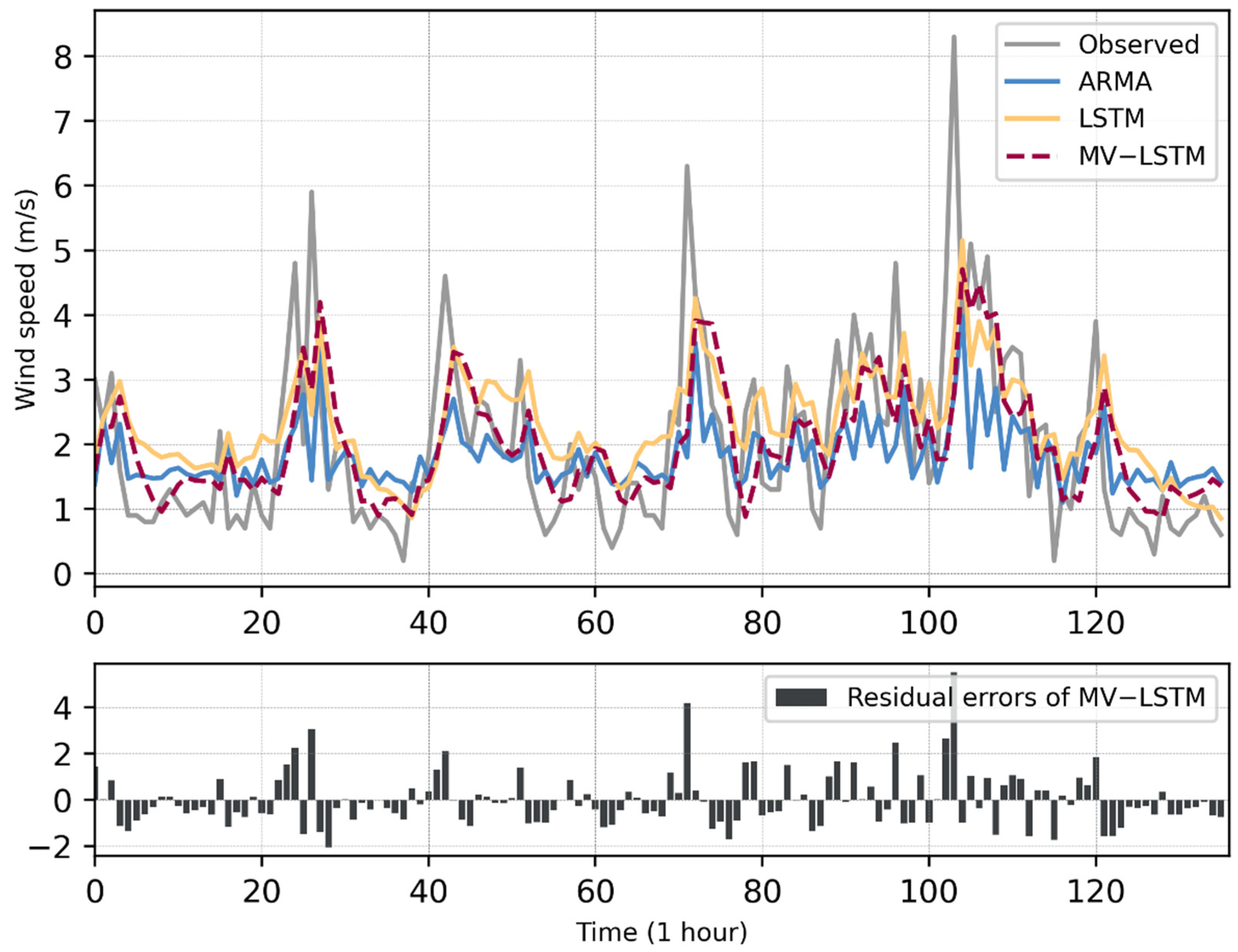
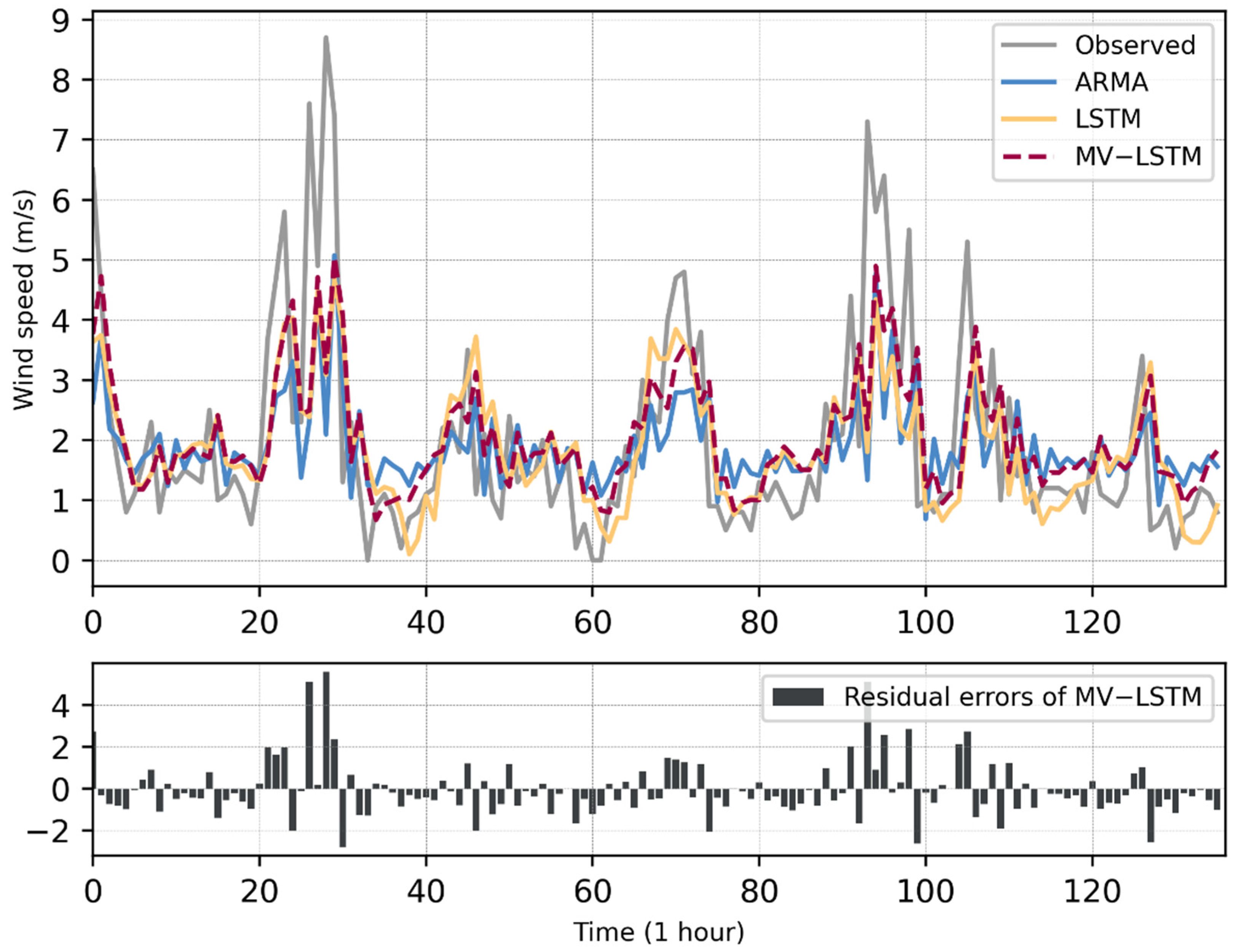
Figure 6 and Figure 7 show the wind speed observations from the test sets of the two stations and the prediction results of the three models. As can be seen in Figure 6, for the data of Yanqing Station, the MV-LSTM model could better predict the minimum value of the wind speed than the LSTM, and could fit the general variation trend of the wind speed better. In Figure 6 and Figure 7, when a wind ramp occurs (which is shown in the figures, the wind speed rises sharply within a short period of time), the prediction residual of the model also increases, which means that the MV-LSTM does not perform well on the maximum point of the wind speed series. In addition, Figure 6 and Figure 7 show that the prediction curves of ARMA, LSTM, and MV-LSTM all have certain hysteresis when compared with the observed data curves. Among these, the sequence of the LSTM method shows obvious hysteresis. The MV-LSTM model could obtain the historical parameters of multiple meteorological elements to represent the wind speed series data in a more complex manner. Therefore, the MV-LSTM model represents an improvement for this problem, but still shows some lag when the wind speed changes sharply.
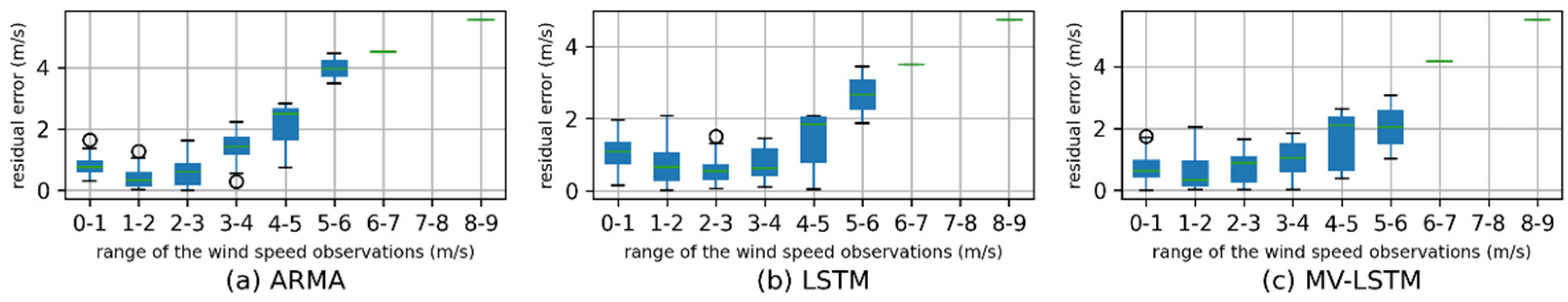
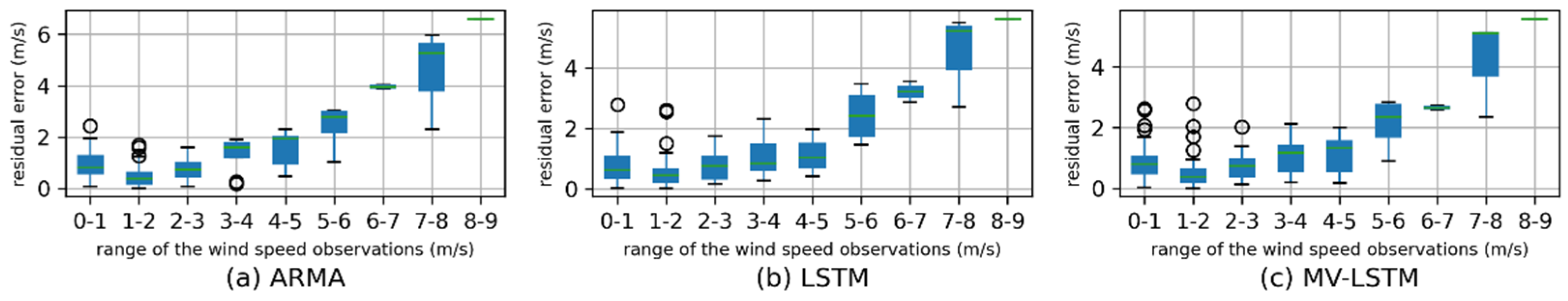
Figure 8 and Figure 9 show residual errors’ distribution of each method in different wind speed observation ranges. The x-axis represents the range of the wind speed observations, and each sub-graph displays the residual error distribution of one method. For each method, the residual error increases as the wind speed increases, which means the prediction performance of each method decreased with the increase in the wind speed. For each station, compared with the other two methods, the predicted residual increase range of the MV-LSTM model is the smallest. For Yanqing Station, when the wind speed is in the range 0–5 m/s, the residual errors of the MV-LSTM method are mostly kept below 2 m/s, which could not be achieved by the other two methods.
4. Conclusions
In this paper, we proposed a multi-variable long short-term memory (MV-LSTM) network model for predicting short-term wind speed. The model can combine the historical data of several meteorological elements to forecast the short-term wind speed. The feasibility of this method was verified on an hourly observation dataset taken from observation stations in Yanqing and Zhaitang from 1 August 2020 to 31 August 2020. The experimental results proved that the prediction performance of the MV-LSTM model is superior to that of the traditional ARMA method and the single-variable LSTM network method based on only historical wind speed data. The experimental results also shows that the performance of the proposed model is different for different datasets and the predicted data curve lags behind the observed data curve at the maximum values of wind speed. Based on this, we will consider optimizing the learning ability of the model by in-creasing its complexity, such as by adding network layers and combining other neural networks, thus improving the model’s prediction accuracy for wind speeds with larger instability and volatility.
Author Contributions
Conceptualization, A.X., H.Y., and J.C.; methodology, A.X. and H.Y.; software, A.X.; supervision, H.Y.; validation, L.S.; writing—original draft, A.X.; writing—review and editing, A.X. and Q.Z. All authors have read and agreed to the published version of the manuscript.
Funding
This work was sponsored by the Sichuan Science and Technology Program (2020YFS0355 and 2020YFG0479).
Data Availability Statement
The data presented in this study are available on request from the corresponding author.
Acknowledgments
Special thanks and appreciation are extended to Fajing Chen for his assistance in the Numerical Weather Prediction Center (NWPC) of the CMA.
Conflicts of Interest
The authors declare that they have no conflict of interest to report regarding the present study.
References
- Burton, T. Wind Energy Handbook; Wiley: Hoboken, NJ, USA, 2011. [Google Scholar]
- Hu, Y.L.; Liang, C. A nonlinear hybrid wind speed forecasting model using LSTM network, hysteretic ELM and Differential Evolution algorithm. Energy Conv. Manag. 2018, 173, 123–142. [Google Scholar] [CrossRef]
- Würth, I.; Valldecabres, L.; Simon, E.; Möhrlen, C.; Uzunoğlu, B.; Gilbert, C.; Giebel, G.; Schlipf, D.; Kaifel, A. Minute-Scale Forecasting of Wind Power—Results from the Collaborative Workshop of IEA Wind Task 32 and 36. Energies 2019, 12, 712. [Google Scholar] [CrossRef] [Green Version]
- Wang, J.; Zhang, W.; Wang, J.; Han, T.; Kong, L. A novel hybrid approach for wind speed prediction. Inf. Sci. 2014, 273, 304–318. [Google Scholar] [CrossRef]
- Giebel, G.; Brownsword, R.; Kariniotakis, G.; Denhard, M.; Draxl, C. The State of the Art in Short-Term Prediction of Wind Power A Literature Overview; Technical Report; Technical University of Denmark (DTU): Roskilde, Denmark, 2011. [Google Scholar] [CrossRef]
- Wang, J.; Zhang, W.; Li, Y.; Wang, J.; Dang, Z. Forecasting wind speed using empirical mode decomposition and Elman neural network. Appl. Soft Comput. 2014, 23, 452–459. [Google Scholar] [CrossRef]
- Chen, D.H.; Xue, J.S. Present situation and prospect of numerical weather forecast business model. Acta Meteorol. Sin. 2004, 623–633. [Google Scholar] [CrossRef]
- Liao, D.X. Design of Atmospheric Numerical Models; China Meteorological Press: Beijing, China, 1999. [Google Scholar]
- Han, X.; Chen, F.; Cao, H.; Li, X.; Zhang, X. Short-term wind speed prediction based on LS-SVM. In Proceedings of the 10th World Congress on Intelligent Control and Automation, Beijing, China, 6–8 July 2012; pp. 3200–3204. [Google Scholar]
- Poggi, P.; Muselli, M.; Notton, G.; Cristofari, C.; Louche, A. Forecasting and simulating wind speed in Corsica by using an autoregressive model. Energy Convers. Manag. 2003, 44, 3177–3196. [Google Scholar] [CrossRef]
- Kavasseri, R.G.; Seetharaman, K. Day-ahead wind speed forecasting using f-ARIMA models. Renew Energy 2009, 34, 1388–1393. [Google Scholar] [CrossRef]
- Lydia, M.; Kumar, S.S.; Selvakumar, A.I.; Kumar, G.E.P. Linear and non-linear autoregressive models for short-term wind speed forecasting. Energy Convers. Manag. 2016, 112, 115–124. [Google Scholar] [CrossRef]
- Du, P.; Wang, J.; Guo, Z.; Yang, W. Research and application of a novel hybrid forecasting system based on multi-objective optimization for wind speed forecasting. Energy Convers. Manag. 2017, 150, 90–107. [Google Scholar] [CrossRef]
- Würth, I.; Ellinghaus, S.; Wigger, M.; Niemeier, M.J.; Clifton, A.; Cheng, P.W. Forecasting wind ramps: Can long-range lidar increase accuracy? J. Physics Conf. Ser. 2018, 1102, 012013. [Google Scholar] [CrossRef] [Green Version]
- Valldecabres, L.; Peña, A.; Courtney, M.; Von Bremen, L.; Kuhn, M. Very short-term forecast of near-coastal flow using scanning lidars. Wind. Energy Sci. 2018, 3, 313–327. [Google Scholar] [CrossRef] [Green Version]
- Ren, C.; An, N.; Wang, J.; Li, L.; Hu, B.; Shang, D. Optimal parameters selection for BP neural network based on particle swarm optimization: A case study of wind speed forecasting. Knowledge-Based Syst. 2014, 56, 226–239. [Google Scholar] [CrossRef]
- Baran, S. Probabilistic wind speed forecasting using Bayesian model averaging with truncated normal components. Comput. Stat. Data Anal. 2014, 75, 227–238. [Google Scholar] [CrossRef] [Green Version]
- Santhosh, M.; Venkaiah, C.; Kumar, D.V. Ensemble empirical mode decomposition based adaptive wavelet neural network method for wind speed prediction. Energy Convers. Manag. 2018, 168, 482–493. [Google Scholar] [CrossRef]
- Zhang, C.; Zhou, J.; Li, C.; Fu, W.; Peng, T. A compound structure of ELM based on feature selection and parameter optimization using hybrid backtracking search algorithm for wind speed forecasting. Energy Convers. Manag. 2017, 143, 360–376. [Google Scholar] [CrossRef]
- Cao, Q.; Ewing, B.T.; Thompson, M.A. Forecasting wind speed with recurrent neural networks. Eur. J. Oper. Res. 2012, 221, 148–154. [Google Scholar] [CrossRef]
- Chen, N.; Xialihaer, N.; Kong, W.; Ren, J. Research on Prediction Methods of Energy Consumption Data. J. New Media 2020, 2, 99–109. [Google Scholar] [CrossRef]
- Zhou, H.; Chen, Y.; Zhang, S. Ship Trajectory Prediction Based on BP Neural Network. J. Artif. Intell. 2019, 1, 29–36. [Google Scholar] [CrossRef]
- Guo, Z.; Zhang, L.; Hu, X.; Chen, H. Wind Speed Prediction Modeling Based on the Wavelet Neural Network. Intell. Autom. Soft Comput. 2020, 26, 625–630. [Google Scholar] [CrossRef]
- Chen, M.-R.; Zeng, G.-Q.; Lu, K.-D.; Weng, J. A Two-Layer Nonlinear Combination Method for Short-Term Wind Speed Prediction Based on ELM, ENN, and LSTM. IEEE Internet Things J. 2019, 6, 6997–7010. [Google Scholar] [CrossRef]
- Fang, W.; Zhang, F.; Ding, Y.; Sheng, J. A new Sequential Image Prediction Method Based on LSTM and DCGAN. Comput. Mater. Contin. 2020, 64, 217–231. [Google Scholar] [CrossRef]
- Yan, B.; Tang, X.; Wang, J.; Zhou, Y.; Zheng, G.; Zou, Q.; Lu, Y.; Liu, B.; Tu, W.; Xiong, N. An Improved Method for the Fitting and Prediction of the Number of COVID-19 Confirmed Cases Based on LSTM. Comput. Mater. Contin. 2020, 64, 1473–1490. [Google Scholar] [CrossRef]
- Liu, H.; Mi, X.; Li, Y. Smart multi-step deep learning model for wind speed forecasting based on variational mode decomposition, singular spectrum analysis, LSTM network and ELM. Energy Convers. Manag. 2018, 159, 54–64. [Google Scholar] [CrossRef]
- Chen, J.; Zeng, G.-Q.; Zhou, W.; Du, W.; Lu, K. Wind speed forecasting using nonlinear-learning ensemble of deep learning time series prediction and extremal optimization. Energy Convers. Manag. 2018, 165, 681–695. [Google Scholar] [CrossRef]
- Nerlove, M.; Diebold, F.X. Autoregressive and Moving-average Time-series Processes. In Time Series and Statistics; Eatwell, J., Milgate, M., Newman, P., Eds.; Palgrave Macmillan UK: London, UK, 1990; pp. 25–35. [Google Scholar]
- Yan, B.Z.; Sun, J.; Wang, X.Z.; Han, N.; Liu, B. Groundwater level prediction based on multivariable LSTM neural network. J. Jilin Univ. 2020, 50, 1. [Google Scholar]
- Ma, X.; Tao, Z.; Wang, Y.; Yu, H.; Wang, Y. Long short-term memory neural network for traffic speed prediction using remote microwave sensor data. Transp. Res. Part. C Emerg. Technol. 2015, 54, 187–197. [Google Scholar] [CrossRef]
- Hochreiter, S.; Schmidhuber, J. Long short-term memory. Neural Comput. 1997, 9, 1735–1780. [Google Scholar] [CrossRef]
- Liang, S.; Nguyen, L.; Jin, F. A Multi-variable Stacked Long-Short Term Memory Network for Wind Speed Forecasting. IEEE Int. Conf. Big Data 2018, 4561–4564. [Google Scholar] [CrossRef] [Green Version]
- Zhou, Z.H. Machine Learning; Tsinghua University Press: Beijing, China, 2016. [Google Scholar]
- Lange, M.; Waldl, H.P. Assessing the uncertainty of wind power predictions with regard to specific weather situations. In Proceedings of the European Wind Energy Conference, Copenhagen, Denmark, 2–6 July 2001; pp. 695–698. [Google Scholar]
- Pearson, K. Notes on the History of Correlation. Biometrika 1920, 13, 25. [Google Scholar] [CrossRef]
- Stigler, S.M. Francis Galton’s Account of the Invention of Correlation. Stat. Sci. 1989, 4, 73–79. [Google Scholar] [CrossRef]
- Song, Z.; Jiang, Y.; Zhang, Z. Short-term wind speed forecasting with Markov-switching model. Appl. Energy 2014, 130, 103–112. [Google Scholar] [CrossRef]
- Li, G.; Shi, J. On comparing three artificial neural networks for wind speed forecasting. Appl. Energy 2010, 87, 2313–2320. [Google Scholar] [CrossRef]
Figure 1.
Geographical location of the stations in Beijing, Northeast China.

Figure 2.
Real meteorological data from Yanqing station.

Figure 3.
Real meteorological data from Zhaitang station.

Figure 4.
LSTM cell structure.

Figure 5.
The framework of the proposed multi-variable LSTM network method for wind speed forecasting.
Figure 5.
The framework of the proposed multi-variable LSTM network method for wind speed forecasting.

Figure 6.
The wind speed forecasting results obtained by the different models on the dataset of Yanqing Station. In the top sub-figure, the x-axis is the wind speed value (unit: m/s), and the y-axis is the time of the data points (time interval: 1 h); in the bottom sub-figure, the x-axis is the residual errors of the MV-LSTM method (unit: m/s), and the y-axis is the same as it in the top sub-figure.

Figure 7.
The wind speed forecasting results obtained by the different models on the dataset of Zhaitang Station. In the top sub-figure, the x-axis is the wind speed value (unit: m/s), and the y-axis is the time of the data points (time interval: 1 h); in the bottom sub-figure, the x-axis is the residual errors of the MV-LSTM method (unit: m/s), and the y-axis is the same as it in the top sub-figure.

Figure 8.
Boxplot of the residual errors of each method with different ranges of the wind speed on the test set of Yanqing Station.
Figure 8.
Boxplot of the residual errors of each method with different ranges of the wind speed on the test set of Yanqing Station.

Figure 9.
Boxplot of the residual errors of each method with different ranges of the wind speed on the test set of Zhaitang Station.
Figure 9.
Boxplot of the residual errors of each method with different ranges of the wind speed on the test set of Zhaitang Station.


Table 1.
Geographical coordinates of the stations.
| Station | Station ID | Longitude (°E) | Latitude (°N) | Altitude(m) |
|---|---|---|---|---|
| Yanqing | 54406 | 115.97 | 40.45 | 487.9 |
| Zhaitang | 54501 | 115.68 | 39.97 | 440.3 |
Table 2.
The statistical wind speed information for the dataset from Yanqing station and Zhaitang station.
Table 2.
The statistical wind speed information for the dataset from Yanqing station and Zhaitang station.
| Station | Dataset | Max | Median | Min | Mean | Standard Deviation |
|---|---|---|---|---|---|---|
| Yanqing | Entire dataset | 8.30 | 1.35 | 0.00 | 1.75 | 1.24 |
| Training dataset | 7.00 | 1.30 | 0.00 | 1.72 | 1.20 | |
| Test dataset | 8.30 | 1.40 | 0.20 | 1.92 | 1.36 | |
| Zhaitang | Entire dataset | 8.70 | 1.50 | 0.00 | 1.87 | 1.42 |
| Training dataset | 8.20 | 1.50 | 0.00 | 1.83 | 1.33 | |
| Test dataset | 8.70 | 1.30 | 0.00 | 2.02 | 1.71 |
Table 3.
The hyper-parameters of the LSTM network model (with one hidden layer).
| Parameter | Value |
|---|---|
| epoch size | 30 |
| batch size | 4 |
| neuron size | 6 |
| loss function | mean squared error (MSE) |
| optimizer | adaptive moment estimation (ADAM) |
Table 4.
Correlation of variables with wind speed (* indicates that the meteorological element is related to wind speed with a p-value of less than 5%).
Table 4.
Correlation of variables with wind speed (* indicates that the meteorological element is related to wind speed with a p-value of less than 5%).
| Yanqing Station | Zhaitang Station | |||
|---|---|---|---|---|
| Correlation | p-Value | Correlation | p-Value | |
| Temperature | 0.37 * | 0.00 | 0.50 * | 0.00 |
| Pressure | −0.08 * | 0.03 | −0.14 * | 0.00 |
| Humidity | −0.09 * | 0.02 | 0.01 | 0.78 |
| Min T | 0.37 * | 0.00 | 0.51 * | 0.00 |
| Max T | 0.39 * | 0.00 | 0.52 * | 0.00 |
| Precipitation in One Hour | 0.01 | 0.70 | −0.00 | 0.99 |
Table 5.
The evaluation metric values for three models on the test set of Yanqing Station.
| Method | RMSE (m/s) | MAE (m/s) | MBE (m/s) | MAPE (%) |
|---|---|---|---|---|
| ARMA | 1.2287 | 0.8853 | −0.1548 | 0.6615 |
| LSTM | 1.1477 | 0.9132 | 0.3170 | 0.7910 |
| MV-LSTM | 1.1460 | 0.8468 | 0.0276 | 0.6412 |
Table 6.
The evaluation metric values for three models on the test set of Zhaitang Station.
| Method | RMSE (m/s) | MAE (m/s) | MBE (m/s) | MAPE (%) |
|---|---|---|---|---|
| ARMA | 1.4638 | 1.0277 | −0.0764 | 0.73611 |
| LSTM | 1.3622 | 0.9343 | −0.1040 | 0.65081 |
| MV-LSTM | 1.3270 | 0.9375 | 0.0602 | 0.68880 |
Publisher’s Note: MDPI stays neutral with regard to jurisdictional claims in published maps and institutional affiliations. |
© 2021 by the authors. Licensee MDPI, Basel, Switzerland. This article is an open access article distributed under the terms and conditions of the Creative Commons Attribution (CC BY) license (https://creativecommons.org/licenses/by/4.0/).
Share and Cite
MDPI and ACS Style
Xie, A.; Yang, H.; Chen, J.; Sheng, L.; Zhang, Q. A Short-Term Wind Speed Forecasting Model Based on a Multi-Variable Long Short-Term Memory Network. Atmosphere 2021, 12, 651. https://0-doi-org.brum.beds.ac.uk/10.3390/atmos12050651
AMA Style
Xie A, Yang H, Chen J, Sheng L, Zhang Q. A Short-Term Wind Speed Forecasting Model Based on a Multi-Variable Long Short-Term Memory Network. Atmosphere. 2021; 12(5):651. https://0-doi-org.brum.beds.ac.uk/10.3390/atmos12050651
Chicago/Turabian StyleXie, Anqi, Hao Yang, Jing Chen, Li Sheng, and Qian Zhang. 2021. "A Short-Term Wind Speed Forecasting Model Based on a Multi-Variable Long Short-Term Memory Network" Atmosphere 12, no. 5: 651. https://0-doi-org.brum.beds.ac.uk/10.3390/atmos12050651
Note that from the first issue of 2016, this journal uses article numbers instead of page numbers. See further details here.