
Atmospheric Wind Field Modelling with OpenFOAM for Near-Ground Gas Dispersion

1
Bundesanstalt für Materialforschung und—Prüfung (BAM), 12205 Berlin, Germany
2
Fakultät für Mathematik, Informatik und Naturwissenschaften, Meteorologisches Institut, Universität Hamburg, 20146 Hamburg, Germany
*
Author to whom correspondence should be addressed.
Atmosphere 2021, 12(8), 933; https://0-doi-org.brum.beds.ac.uk/10.3390/atmos12080933
Submission received: 2 July 2021
/
Revised: 14 July 2021
/
Accepted: 15 July 2021
/
Published: 21 July 2021
(This article belongs to the Special Issue High Performance Computing Serving Atmospheric Transport & Dispersion Modelling)
Abstract
:CFD simulations of near-ground gas dispersion depend significantly on the accuracy of the wind field. When simulating wind fields with conventional RANS turbulence models, the velocity and turbulence profiles specified as inlet boundary conditions change rapidly in the approach flow region. As a result, when hazardous materials are released, the extent of hazardous areas is calculated based on an approach flow that differs significantly from the boundary conditions defined. To solve this problem, a turbulence model with consistent boundary conditions was developed to ensure a horizontally homogeneous approach flow. Instead of the logarithmic vertical velocity profile, a power law is used to overcome the problem that with the logarithmic profile, negative velocities would be calculated for heights within the roughness length. With this, the problem that the distance of the wall-adjacent cell midpoint has to be higher than the roughness length is solved, so that a high grid resolution can be ensured even in the near-ground region which is required to simulate gas dispersion. The evaluation of the developed CFD model using the German guideline VDI 3783/9 and wind tunnel experiments with realistic obstacle configurations showed a good agreement between the calculated and the measured values and the ability to achieve a horizontally homogenous approach flow.
1. Introduction
When assessing hazards from industrial plant applications, calculating the gas dispersion is one of the main tasks for determining safety distances. Simple models for calculating the gas dispersion are generally not able to account for obstacles such as buildings or the topography of the dispersion area. To simulate dispersion scenarios in complex areas, computational fluid dynamics (CFD) codes can be used. By solving the full Navier–Stokes equations, CFD codes can simultaneously model the wind field and the dispersion of pollutants, taking into account obstacles, topography, and thermal stratification, as well as the type of release (with or without momentum). Simulating gas dispersion is mainly influenced by the wind field. The main problem when using CFD codes is the cost–benefit ratio, as the computational time is exceedingly high compared to simpler models. To reduce the computational time, relying on RANS (Reynolds-averaged Navier–Stokes) equations is a common practice. To close the RANS equations, the - turbulence model is used in a wide number of publications for calculating the atmospheric wind field.
When simulating near-ground atmospheric boundary layer phenomena, fully developed wind and turbulence profiles are specified as inlet boundary conditions. Due to numerical reasons, every CFD simulation requires a computational domain of spatial extensions much above the dimensions of the area of interest. Therefore, an obstacle free approach flow region is required between the inlet and the first obstacle [1]. To ensure that the posed inlet boundary conditions reach the area of interest, where the release and dispersion occurs, a CFD model should be chosen that is able to conserve the inlet conditions in the approach flow region, resulting in a horizontally homogenous boundary layer flow. Otherwise, the turbulence model of the CFD code will modify the approach flow depending on the domain length and grid resolution, resulting in different extents of hazardous areas for the same release scenario [2].
Several publications [3,4,5,6] state that reaching a horizontally homogenous boundary layer flow with RANS CFD models is not evident. Richards and Hoxey [7] state that a horizontally homogenous boundary layer flow can only be reached if there is a consistency between the turbulence model and the boundary conditions, such as the atmospheric inlet condition and wall functions. They propose inlet conditions on the basis of a logarithmic wind profile, as well as necessary modifications to the - turbulence model. Several other authors [8,9,10] present comparable solutions for the problem of horizontal homogeneity. Whilst all aforementioned publications try to achieve a solution by modifying the constants of the - model, [11] they achieved the horizontal homogeneity by introducing an additional source term to the dissipation equation [12] and by introducing it in the turbulent kinetic energy equation.
To reduce the computational cost, wall functions are used for describing the near wall area using a roughness factor, to avoid modelling even the smallest details (e.g., vegetation, fences, cars). Different types of roughness parameters and their suitability for modelling horizontally homogenous boundary layer flows were discussed [13,14,15]. However, for all it was stated that the general formulations of wall functions for rough walls (based on the equivalent sand grain roughness or the roughness length ) introduce a dependency of the wall-adjacent cell size from the defined roughness value. This results in wall-adjacent cell sizes that are much too big for simulating near-ground or near-obstacle effects with acceptable accuracy. If a near-wall cell size smaller than the requirements due to the defined roughness is chosen, the simulation will not result in a horizontally homogenous boundary layer flow [13].
For near-ground gas dispersion scenarios, a coarse wall-adjacent mesh will lead to an unrealistic prediction of the gas cloud sizes, as the concentration gradients near ground cannot be resolved with sufficient accuracy.
In this work, a CFD model based on the open source CFD code OpenFOAM is presented, which was developed with the aim to compute a horizontally homogenous boundary layer flow and to overcome the wall resolution restrictions due to wall roughness. In this model the wind profile is described by a power law instead of a log wind profile. The used flow solver is a transient, compressible flow solver, to also be able to simulate in the future gas dispersion, gas cloud explosions, or gas cloud combustion. In this work we will focus on the wind field modelling. The model will be evaluated systematically using the German Guideline VDI 3783/9 [16,17]. This guideline provides test cases in which generic obstacle configurations are investigated and objective evaluation criteria are provided. To evaluate the model performance for a more realistic obstacle configuration comparable to an industrial area, wind tunnel measurements are used. In opposite to free field trials, they show a high reproducibility, and the average boundary conditions can be kept constant over a long time period to produce a statistically sound database. The wind tunnel data used were generated at the University of Hamburg in the context of an actual research project. The quality of the presented model to simulate a horizontally homogenous boundary layer approach flow and the flow around obstacles will be demonstrated and evaluated with the VDI Guideline 3783/9 and the aforementioned wind tunnel experiments.
2. Turbulence Model and Boundary Conditions for Neutral Stratification
The presented CFD model is based on the transient and compressible solver rhoReactingBuoyantFoam [18,19], as well as on the --turbulence model of Launder and Spalding [20] and El Tahry [21], implemented in OpenFOAM 5.0. The differential equations describing the turbulent kinetic energy (1) and the dissipation (2) are coupled to the Navier–Stokes equations through the turbulent viscosity (3):
The values of the model constants , , , and in Equations (1)–(3) are based on [22]. The variable is the density of the fluid and is the velocity vector, describes the production of the turbulent kinetic energy and is an additional source term, which will be derived in the following.
With the idealized assumption of a horizontally homogenous boundary layer flow and with the additional assumptions that:
- -
- the flow is stationary,
- -
- the flow fields are free of horizontal gradients,
- -
- the vertical velocity is zero,
Equations (1) and (2) can be simplified to:
The dynamic viscosity is assumed to be negligible ( ).
Assuming a two-dimensional horizontally homogenous boundary layer flow, the turbulence production is defined as
Based on Equations (4) to (6), models have been developed to achieve a horizontally homogenous boundary layer solution (e.g., [7,10,12]). All these models are based on a logarithmic wind velocity profile. This assumption leads to a dependency of the grid resolution near ground from the roughness length [13]. To overcome this restriction, in this work a power-law wind profile is used as inlet boundary condition
The value of the exponent m of the wind profile is set in accordance to the roughness length z0, which is now only indirectly linked to the governing model equations, allowing us to choose the grid resolution independently of the ground roughness.
The vertical profile of the turbulent kinetic energy of the incident flow, as described by, e.g., Richards and Hoxey [7], is dependent on the wall shear stress velocity which can be defined as nearly constant with height for a neutrally layered atmosphere
To achieve a horizontally homogenous atmospheric boundary layer flow, it is mandatory that the flow profiles at the inlet boundary satisfy the equations of the turbulence model. This is achieved for the turbulent kinetic energy Equation (4) with the condition that for
From Equations (3), (6)–(8), and (10), the vertical profile of the turbulent dissipation ε at the inlet boundary is
The inlet boundary conditions (7), (8), and (11) only satisfy the equation for the turbulent dissipation (5) with
With this modification, horizontally homogenous boundary layer flows can be simulated for near-ground grid resolutions that are not dependent on the roughness length. This source term is evaluated solely based on the vertical inlet profiles at the beginning of the simulation and is therefore time independent. As this source term is relevant and designed to achieve a horizontally homogenous flow without obstacles, this term is only active in the upstream region when simulating obstacles in the domain. In the vicinity of obstacles, the turbulence model (Equations (1)–(3)) is used with . The term compensates the expected dissipation of turbulent kinetic energy with the standard k-ϵ-model in an obstacle-free flow domain.
Besides the described modifications to the turbulence model, the simulation of a horizontally homogenous boundary layer flow also requires a formulation for wall functions consistent to the modifications made. Wall functions available in OpenFOAM describe the turbulent energy dissipation and production for hydraulically smooth walls (epsilonWallFunction), as well as the turbulent viscosity based on the roughness length (nutkAtmRoughWallFunction). To avoid reintroducing here the dependency of the possible grid resolution on the roughness length, and at the same time to satisfy Equation (11), the turbulent dissipation at the wall-adjacent cell center is defined as
Coupling of the wall function with the flow field occurs in analogy to the OpenFOAM epsilonWallFunction [18], by replacing the friction velocity by the wall adjacent turbulent kinetic energy through Equation (8)
In accordance with Equation (6), the turbulence production in the wall adjacent cell is
In analogy to the OpenFOAM nutkAtmRoughWallFunction [18], one of the two velocity gradients of the wall function is replaced by the analytical derivative of the power law profile and the other by its spatial discretization. Thus, the turbulence production can be rewritten as
The wall sheer stress , considered as constant within the Prandtl layer, is
and by integration with respect to the height and assuming a no slip wall, Equation (17) becomes
resulting in the wall function for the turbulent viscosity, by substituting up with Equation (7):
For the turbulent kinetic energy, a zero gradient is specified at the wall, in accordance with the inlet boundary condition.
Studies [13,23] observed that choosing fixed shear stress as a boundary condition on the top of the domain instead of a symmetry boundary condition leads to a less inhomogeneous horizontal boundary layer. This was also confirmed by [24] who noticed a better agreement with experimental values when setting a fixed shear stress as the top boundary condition. Therefore, in the presented model, constant values for the wind speed and the turbulent values based on Equations (7)–(9) are set as the top boundary conditions. All other values are set to zero gradient.
3. Results
Several investigations have been carried out to assess the accuracy of the presented model. Beginning with a study of the horizontal homogeneity of the boundary layer flow when using the original and the modified code over a benchmark with the VDI 3783/9 [16,17], to a comparison with wind tunnel experiments for complex terrain, the quality of the new model is shown.
3.1. Horizontally Homogeneous Boundary Layer
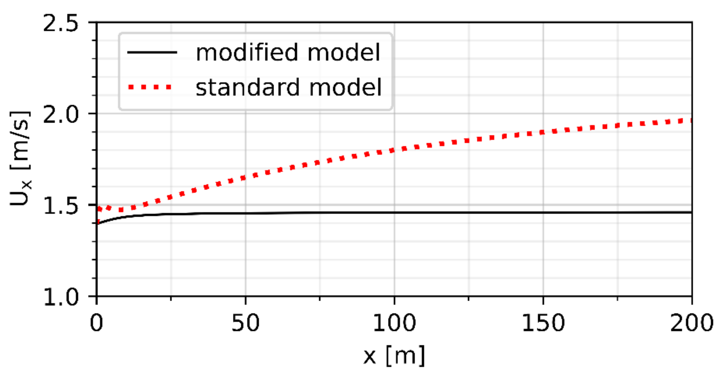
By using a power law to describe the vertical velocity profile and introducing the additional source term , it should be possible to simulate a horizontally homogenous boundary layer flow with a grid resolution not depending on the roughness length. Figure 1 shows the wind velocity in the main direction calculated by the - turbulence model without modification (standard model) and with the model presented here (modified model) at a height of 1 m above the ground from the inlet up to a distance of 200 m. A power law with a reference velocity of 3 m/s at a reference height of 10 m was specified as the inlet boundary condition and a roughness length of 1.2 m was assumed. For the standard model, a wall function based on the roughness length is chosen (OpenFOAM nutkAtmRoughWallFunction), whilst the roughness length is approximated by the exponent of the power law in the modified model. The simulations were carried out in a 400 m × 8 m × 100 m (l × w × h) pseudo 2D domain without obstacles. In Figure 1, it can be clearly seen that the standard model, as expected, does not conserve the wind profile over the distance, whereas the modified model shows insignificant deviations from the given inlet velocity.
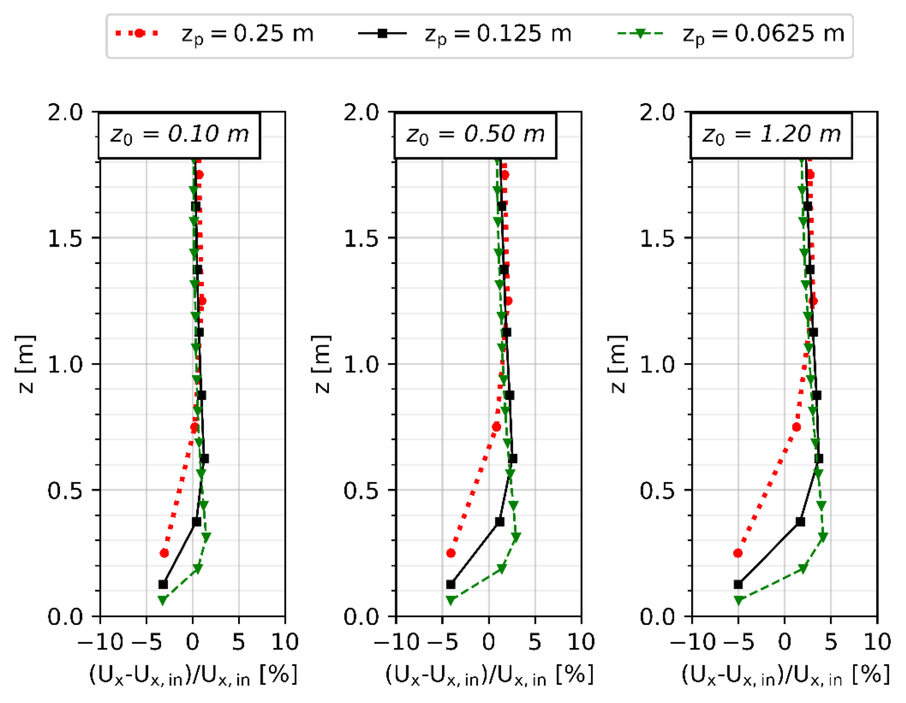
To ensure the presented model being able to carry out simulations of a horizontally homogenous boundary layer flow where the grid resolution can be chosen independently of the surface roughness, which is not possible for standard turbulence models in CFD [13], further simulations were carried out in the same domain. In these simulations, the wind speed at 10 m in height over the ground was varied in a range of 1 m/s up to 5 m/s, and for wind profiles corresponding to roughness lengths between 0.1 m and 1.2 m, covering a typical range for hazard assessment scenarios. The wind profiles were investigated after a distance of 300 m, a typical distance from the inlet according to the best practice guidelines [1], where distances from the inlet of two to eight times the obstacle height are recommended as the approach flow distance. The grid resolution ranged from 0.5 m down to 0.125 m for the wall-adjacent cell, corresponding to cell midpoint heights of 0.25 m down to 0.0625 m.
Figure 2 shows the relative deviation between the calculated vertical wind profile in the main direction () and the inlet boundary condition. As no significant changes were observed over the range of wind speeds, the figure shows exemplarily the results for a wind speed of 3 m/s at 10 m over the ground. The wind profiles after the investigated distance of 300 m do not differ from the inlet profile by more than +/−5% close to the ground. At a height of 1 m or more from the ground, the deviation between the inlet profile and the computed values is negligible. Similar observations can be made for the eddy viscosity profiles (Figure 3). The maximum deviation reached is around +/−10%, which seems small enough to be qualified as acceptable.
As these observations for the wind velocity and eddy viscosity profiles are valid for any of the investigated combinations of roughness length and grid resolution, it can be concluded that the modified turbulence model and wall functions presented here are able to simulate a horizontally homogenous boundary layer flow for near-wall grid resolutions that can be chosen independently to the roughness length.
3.2. VDI 3783/9 Benchmark
The German Guideline VDI 3783/9 [16,17] is used to evaluate the quality of wind field models for a built-up environment. In the guideline, a number of test cases are defined to evaluate different characteristics of the wind field model. In some test cases, comparisons of the model have to be performed with wind tunnel experiments that were carried out for generic obstacle configurations (scale 1:200) by the meteorological institute of the University of Hamburg [25]. As the aim of this work is to provide a wind field model for, e.g., dispersion scenarios in built up environment, the evaluation of the model presented here is carried out with these test cases.
The evaluation method of the guideline VDI 3783/9 gives a quantitative estimate of the model quality by determining a hit ratio
It indicates in percent the proportion of the total of correctly predicted values in the total number of comparison values N. For successful validation in comparison with wind tunnel experiments, it is required that > 66%. The number of correctly predicted values results from the comparison of the normalized results and the normalized comparison values [17]:
In Equation (22), W is the absolute permitted difference and D the permitted difference, which are defined separately for each case in [16,17].
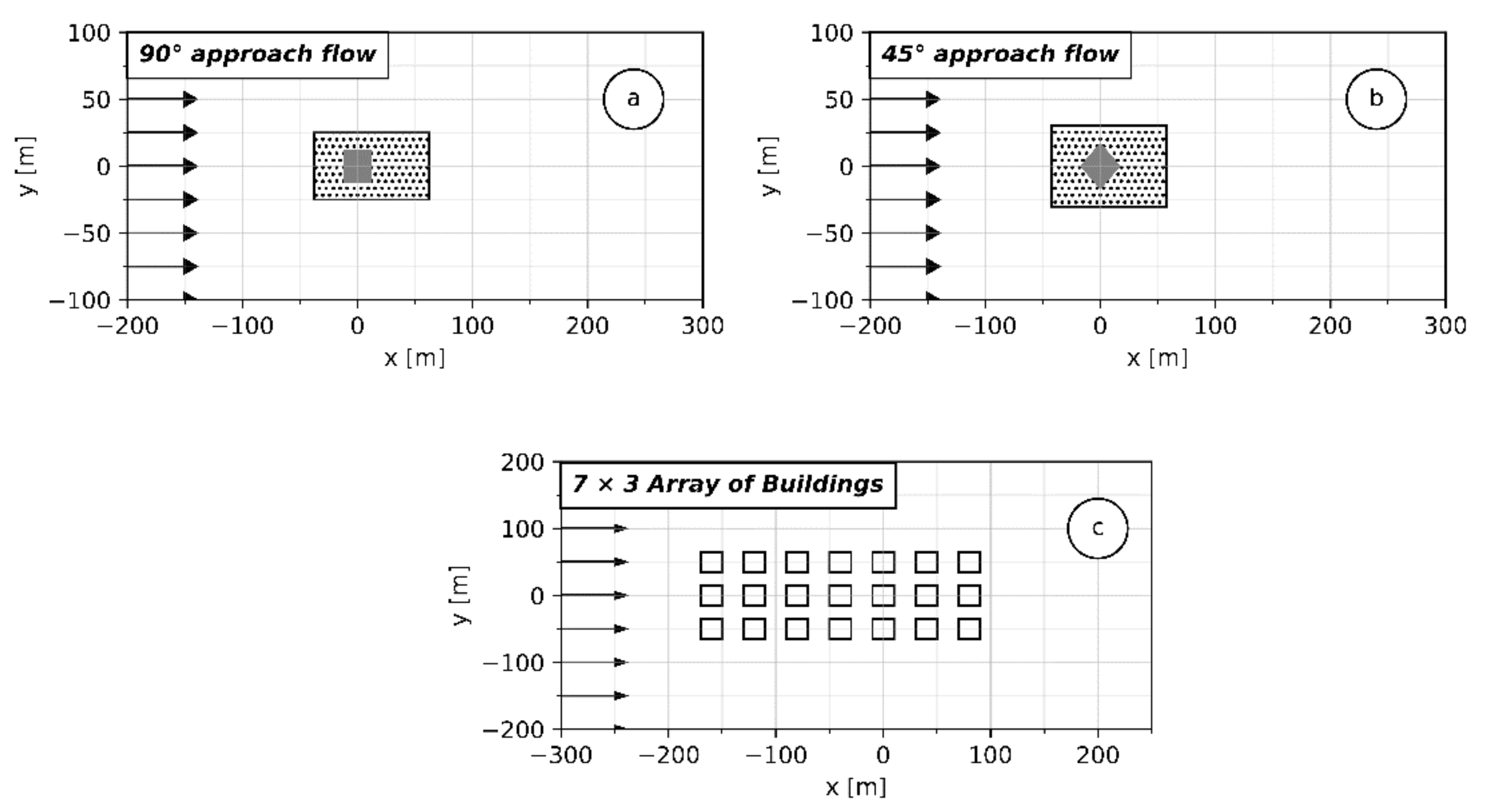
The focus is laid on the test cases c3, c4 and c6 of the 2005 version of the guideline [16], as a simple generic case for a multiple building scenario (test case c6) is available. Figure 4 shows the geometrical representation of the test cases, and the corresponding parameters are given in Table 1. Parameters of each test case. For the test cases c3 and c4 (single obstacle), the guideline requires evaluating the wind field in the near field (grey dotted region in Figure 4a,b), as well as in the whole computational domain. For test case c6, only the whole domain has to be considered.
During a grid sensitivity study, the grid was refined from near-wall mesh sizes of 1.0 m down to 0.25 m, showing that the hit ratio is not very sensitive to the grid refinement, as only negligible differences for all refinements can be observed. In the following, only results for a mesh with a near-wall mesh size of 0.5 m will be discussed, although the observations made are also valid for all investigated meshes.
Table 2 Hit ratio in % for all three test cases. shows the hit ratio for all three test cases, subdivided into hit ratios for —corresponding to the main wind direction, —the crosswind direction, and —the vertical to the main wind direction. For all test cases and all three wind direction components, the required minimum hit ratio of 66% is reached or exceeded when evaluating the whole computational domain.
While the near-field values for test case c3 meet the requirements of the guideline, test case c4 does not reach the required minimum value for the hit ratio for some velocity components. Due to the high velocity gradients occurring at obstacles where a flow detachment or recirculation can be observed, the choice of the turbulence model has a significant influence on the quality of the result, whilst, in general, a higher deviation between computed values and experimental data is to be expected in these cases. Although the minimum criterion for the hit ratio is reached for test case c3, in test case c4 with a 45° approach flow, this can only be achieved for the hit ratio of the main wind direction component. Study [26] stated that the approach flow in the experiments for test case c4 was not exactly 45° but showed a slight deviation of 2°. It is still to be examined whether correcting the simulation values for the 2° deviation might lead to better hit ratios.
3.3. Wind Tunnel Experiments
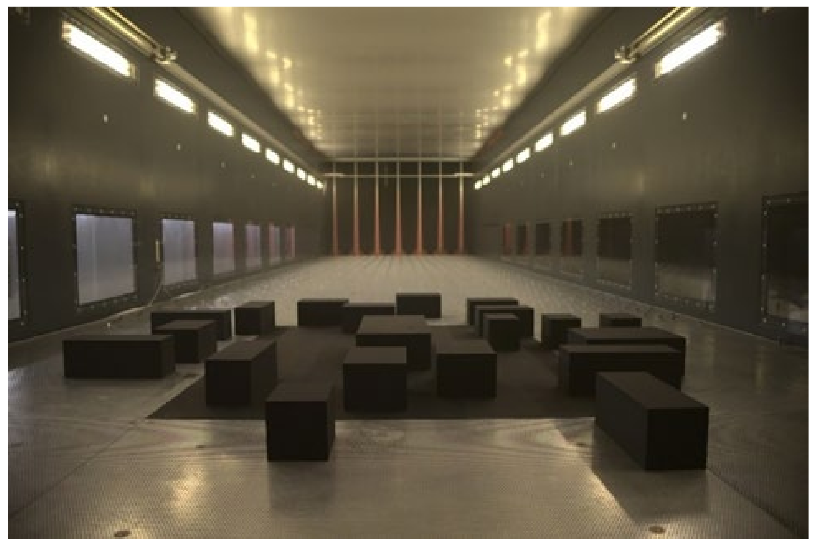
After having compared the model results to such generic cases as the ones defined in [16,17], the model is still to be validated for a more realistic obstacle configuration. Due to the high reproducibility and to a lack of field experiments, wind tunnel data generated at the University of Hamburg in the context of an actual research project are used. The experiments were carried out at the EWTL large boundary layer wind tunnel of the University of Hamburg in a scale of 1:100. The 25 m long wind tunnel has an 18 m long, 4 m wide and approx. 3 m high test section. The investigated model area (Figure 5) was planned with aerial photos and building data from real industrial areas. In real scale, it covers about 300 m × 300 m. The model consists of 20 cuboid shaped buildings which have varying side lengths of 20 m to 40 m. Each building has a height of 15 m. The spaces between the buildings range between 10 m and 80 m. In the middle of the model area, a large building is located. This main building has a base area of 30 m × 60 m. The main building has three openings on the sides and one opening on the roof with a size of 4 m × 4 m. In the future, it is planned to carry out gas dispersion experiments with this setup where the mentioned openings on the buildings will be used as gas inlets.
Flow measurements were performed with Laser-Doppler Anemometry (LDA). The LDA measures two components of the turbulent wind vector simultaneously with a spatial resolution of approx. 110 mm in full scale. To receive statistical representative time series in a turbulent flow, measurements are performed for several minutes. In real scale, this represents a measurement taken for 30 h under stationary meteorological conditions.
Two different boundary layer approach flows are modelled at a scale of 1:100 to investigate the influence of the flow on the measurements inside the model area. One boundary layer flow represents the conditions of a “moderately rough” boundary layer. This type of boundary layer flow develops over grasslands or farmlands. The second wind boundary layer represents a flow that develops over suburban area and is described by the definition of a “rough” boundary layer. The roughness classes are defined by VDI 3783/12 [27]. The similarity between wind tunnel experiments and real scale has been ensured by checking that the turbulence intensity, the wind profiles, the spectral distribution of turbulent energy and the lateral homogeneity are similar to nature-given profiles and distributions. In addition, the functional relationship between the roughness length and the wind profile exponent m has been checked, according to [28].
In the following, the simulated wind fields are compared to the profiles measured in the wind tunnel for the “moderately rough” case. For the considered case, the roughness length for the “moderately rough” case is = 0.06 m, corresponding to an exponent of the wind profile power law of = 0.17. The same approach flow (Figure 6a) was used for two different wind directions, case M1 and case M2 (with respect to the obstacles, Figure 6b). The horizontal flow components (, ) were measured around the obstacles at 327 positions for the direction M1 and at 383 positions for M2, at a height over the ground varying from 2 m up to 20 m. Figure 6a shows a good agreement of the measured and calculated normalized vertical wind velocity profile of the approach flow. For each horizontal, homogeneity was verified.
For the following investigations of the model performance, an objective evaluation method comparable to the VDI Guideline 3783/9 is desirable. In the VDI Guideline 3783/9, in the 2017 version [17], a test case is defined for a real built-up area. The evaluation criteria for this case ( = 25% and = 0.08, threshold for = 66%) are applied to the cases investigated here, as they also represent realistic topographies. It should be noted that the evaluation criteria of the VDI Guideline are defined as case-specific and therefore might not be fully adapted to the cases M1 and M2. Nevertheless, as the permitted differences ( and ) and the hit ratio do not change significantly for all cases of the guideline, this approach appears to be permissible.
For the cases M1 and M2, grid refinements were carried out to investigate if the hit ratio might be independent of the resolution, as this was the case in Section 3.2. For both cases, it is noticed that, with each refinement of the grid, the hit ratio increased up to a point where a grid resolution of 0.25 m adjacent to the obstacles finally led to a successful “validation” in terms of reaching the hit ratio threshold. These simulations already showed a total number of cells > 20 Mio. As further refinement would have led to domains with at least 80 Mio. cells, no further refinement was investigated due to the resulting extremely long simulation time.
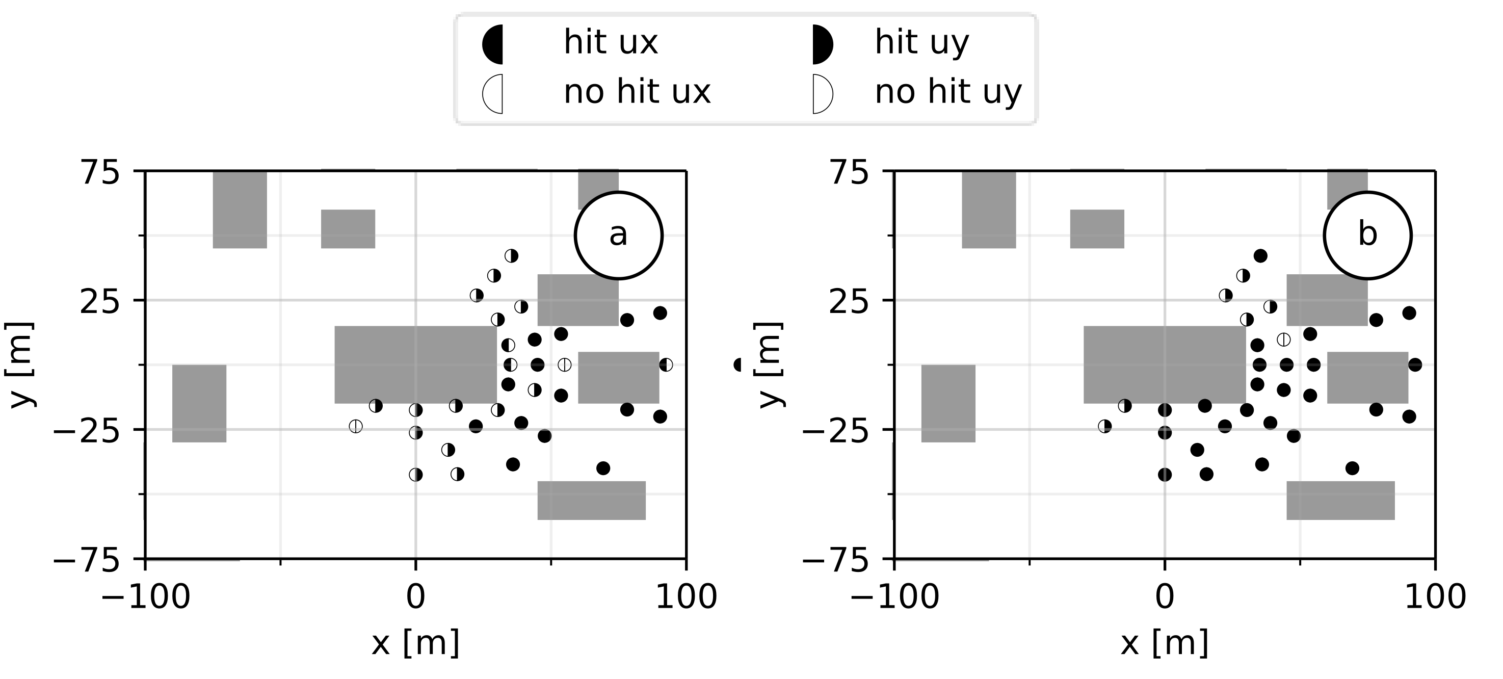
Figure 7 and Figure 8 show the repartition of the measuring points at heights of 2 m (Figure 7a and Figure 8a) and 8 m over the ground (Figure 7b and Figure 8b), respectively, for cases M1 and M2. Whilst in the VDI Guideline the experimental data used to define the thresholds are evenly spread over the whole domain, the measuring points in cases M1 and M2 are concentrated around buildings and close to the ground, making it harder to reach the threshold. Both figures represent the investigated area in such way that the approach flow is oriented parallel to the x-axis coming from the left. Full black bullets show a point where the calculated hit ratios and reach values higher than the threshold of 66%, half-filled bullets show points where the hit ratio of one velocity component did not reach the threshold, and for the blank bullets, no component of the horizontal velocity reached the threshold.
With increasing height over the ground, the number of points which show a hit ratio higher than the threshold increases in both cases. This is due to the fact that the closer to the ground, the more complex the turbulence-influenced effects are on the flow. To resolve these effects in a satisfactory manner, at least a LES (Large-Eddy Simulation) would be required. Table 3 Hit ratio for the whole domain of case M1 and M2. shows that the hit ratio for the whole domain exceeds the threshold value of 66% for both cases. For the aim of providing an adequate wind field for hazard assessment purposes, the reached accuracy is therefore sufficient.
4. Discussion
The transient, compressible flow solver rhoReactingBuoyantFoam of OpenFOAM 5.0 in combination with the standard k-ε turbulence model is promising for simulating the dispersion process of pollutants in the atmosphere. Due to inconsistencies between the required boundary conditions for modelling atmospheric boundary layer flow and the formulation of the turbulence model, simulating a horizontally homogenous boundary layer flow is not possible.
As the horizontally homogenous approach flow is mandatory for reliable estimations of the safety distances for hazard assessment purposes, when a pollutant is released near ground in the atmosphere, a modification to the turbulence model has been made and was presented in this work. Introducing an additional source term in the equation for the turbulent dissipation and replacing the log law profile by a power law profile for the wind field, in combination with a new formulation of the wall functions, showed the ability to simulate a horizontally homogenous boundary layer flow. Additionally, the grid resolution adjacent to the walls can now be chosen independently of the roughness length defined on the ground. For gas dispersion purposes in a built-up domain, the grid resolution in the vicinity of buildings is crucial to achieve a satisfactory resolution of the concentration gradients, leading to a reliable and reproducible prediction of the safety distances. The model’s performance for this application is currently under investigation.
The evaluation of the presented model occurred in three steps. In the first step, it was checked against the original model formulation for its performance to produce horizontally homogenous wind and turbulence profiles, and showed a clear advantage compared to the original formulation by achieving the homogeneity. In the second step, the model was evaluated considering the rules defined by the VDI Guideline 3783/9 [16] where generic obstacle configurations are presented, and an objective statistical method for evaluation using a so-called hit ratio is defined. The model was evaluated against three test cases of the guideline with a single cube in a 90° approach flow and a 45° approach flow, as well as for an array of 7 × 3 obstacles. Considering the whole domain, the model performed well in all cases and reached hit ratios clearly fulfilling the defined threshold. For the two single cube cases, an evaluation of the “near-field” had to be carried out. The hit ratio showed lower values than for the whole domain, due to restrictions of the - turbulence model in the vicinity of obstacles. The third evaluation step consisted of comparing the presented model to wind tunnel measurements and using the evaluation criteria of the VDI Guideline 3783/9 [17] to obtain an objective measure of the performance, even though the criteria might not fully match the considered case. Nevertheless, the presented model showed again a good performance by reaching the required thresholds.
Author Contributions
Conceptualization, S.S. and A.H.; model development and validation, S.S.; wind tunnel measurements, S.M.; All authors were actively involved in writing and revising the manuscript. All authors have read and agreed to the published version of the manuscript.
Funding
The IGF-Project No.: 20719 BG of the Research Association Society for Chemical Engineering and Biotechnology (DECHEMA), Theodor-Heuss-Allee 25, 60486 Frankfurt am Main, was funded by the German Federation of Industrial Research Associations (AiF) within the framework of the Industrial Collective Research (IGF) support program by the Federal Ministry for Economic Affairs and Energy due to a decision of the German Bundestag.
Institutional Review Board Statement
Not applicable.
Informed Consent Statement
Not applicable.
Conflicts of Interest
The authors declare no conflict of interest.
References
- Franke, J.; Hellsten, A.; Schlünzen, H.; Carissimo, B. Best Practice Guideline for the CFD Simulation of Flows in the Urban Environment: COST Action 732 Quality Assurance and Improvement of Microscale Meteorological Models; Meteorological Institute University of Hamburg: Hamburg, Germany, 2007. [Google Scholar]
- Batt, R.; Gant, S.E.; Lacome, J.-M.; Truchot, B. Modelling of stably-stratified atmospheric boundary layers with commercial CFD software for use in risk assessment. Chem. Engineer. Trans. 2016, 48, 61–66. [Google Scholar]
- Richards, P.; Younis, B. Comments on “prediction of the wind-generated pressure distribution around buildings” by E.H. Mathews. J. Wind. Eng. Ind. Aerodyn. 1990, 34, 107–110. [Google Scholar] [CrossRef]
- Quinn, A.D.; Wilson, M.; Reynolds, A.M.; Couling, S.B.; Hoxey, R.P. Modelling the dispersion of aerial pollutants from agricul-tural buildings—An evaluation of computational fluid dynamics (CFD). Comput. Electron. Agric. 2001, 30, 219–235. [Google Scholar] [CrossRef]
- Zhang, C.X. Numerical predictions of turbulent recirculating flows with a k–ε model. J. Wind. Eng. Ind. Aerod. 1994, 51, 177–201. [Google Scholar] [CrossRef]
- Riddle, A.; Carruthers, D.; Sharpe, A.; McHugh, C.; Stocker, J. Comparisons between FLUENT and ADMS for atmospheric dispersion modelling. Atmos. Environ. 2004, 38, 1029–1038. [Google Scholar] [CrossRef]
- Richards, P.J.; Hoxey, R.P. Appropriate boundary conditions for computational wind engineering models using the k-ε mod-el. J. Wind. Eng. Ind. Aerod. 1993, 46–47, 145–153. [Google Scholar] [CrossRef]
- Alinot, C.; Masson, C. k–ε model for the atmospheric boundary layer under various thermal stratifications. J. Sol. Energy Eng. 2005, 127, 438–443. [Google Scholar] [CrossRef]
- Yang, W.; Quan, Y.; Jin, X.; Tamura, Y.; Gu, M. Influences of equilibrium atmosphere boundary layer and turbulence param-eter on wind loads of low-rise buildings. J. Wind. Eng. Ind. Aerodyn. 2008, 96, 2080–2092. [Google Scholar] [CrossRef]
- Yang, Y.; Gu, M.; Chen, S.; Jin, X. New inflow boundary conditions for modelling the neutral equilibrium atmospheric boundary layer in computational wind engineering. J. Wind. Eng. Ind. Aerodyn. 2009, 97, 88–95. [Google Scholar] [CrossRef]
- Pontiggia, M.; Derudi, M.; Busini, V.; Rota, R. Hazardous gas dispersion: A CFD model accounting for atmospheric stability classes. J. Hazard. Mater. 2009, 171, 739–747. [Google Scholar] [CrossRef] [PubMed]
- Van Der Laan, M.P.; Kelly, M.C.; Sørensen, N.N. A new k-epsilon model consistent with Monin-Obukhov similarity theory. Wind. Energy 2016, 20, 479–489. [Google Scholar] [CrossRef] [Green Version]
- Blocken, B.; Stathopoulos, T.; Carmeliet, J. CFD simulation of the atmospheric boundary layer: Wall function problems. Atmos. Environ. 2007, 41, 238–252. [Google Scholar] [CrossRef]
- Zhang, X. CFD Simulation of Neutral ABL Flows; Danmarks Tekniske Universitet, Risø Nationallaboratoriet for Bæredygtig Energi: Kongens Lyngby, Denmark, 2009. [Google Scholar]
- Parente, A.; Gorlé, C.; van Beeck, J.; Benocci, C. Improved k-ε model and wall function formulation for the RANS simula-tion of ABL flows. J. Wind. Eng. Ind. Aerodyn. 2011, 34, 107–110. [Google Scholar]
- Environmental Meteorology—Prognostic Microscale Windfield Models—Evaluation for Flow around Buildings and Obstacles; VDI Guideline 3783, Part 9; Beuth Verlag: Berlin, Germany, 2005.
- Environmental Meteorology—Prognostic Microscale Windfield Models—Evaluation for Flow around Buildings and Obstacles; VDI Guideline 3783, Part 9; Beuth Verlag: Berlin, Germany, 2017.
- OpenFOAM. User Guide. Version 7. OpenFOAM—The OpenFOAM Foundation. 2019. Available online: https://openfoam.org (accessed on 24 July 2020).
- Weller, H.G.; Tabor, G.; Jasak, H.; Fureby, C. A tensorial approach to computational continuum mechanics using ob-ject-oriented techniques. Comput. Phys. 1998, 12, 620–631. [Google Scholar] [CrossRef]
- Launder, B.E.; Spalding, D.B. The numerical computation of turbulent flows. Comput. Method Appl. Mech. Eng. 1974, 3, 269–289. [Google Scholar] [CrossRef]
- El Tahry, S.H. k-epsilon equation for compressible reciprocating engine flows. J. Energy 1983, 7, 345–353. [Google Scholar] [CrossRef]
- Jones, W.; Launder, B. The prediction of laminarization with a two-equation model of turbulence. Int. J. Heat Mass Transf. 1972, 15, 301–314. [Google Scholar] [CrossRef]
- Hargreaves, D.; Wright, N. On the use of the k–ε model in commercial CFD software to model the neutral atmospheric boundary layer. J. Wind. Eng. Ind. Aerodyn. 2007, 95, 355–369. [Google Scholar] [CrossRef]
- Franke, J.; Sturm, M.; Kalmbach, C. Validation of OpenFOAM 1.6.x with the German VDI guideline for obstacle resolving micro-scale models. J. Wind. Eng. Ind. Aerodyn. 2012, 104–106, 350–359. [Google Scholar] [CrossRef]
- Leitl, B. Compilation of Experimental Data for Validation of Micro Scale Dispersion Models (CEDVAL). Available online: https://mi-pub.cen.uni-hamburg.de/index.php?id=433 (accessed on 1 May 2021).
- Eichhorn, J. MISKAM Version 5.02—Evaluierung nach VDI-RL 3783/9. Available online: http://www.lohmeyer.de/ (accessed on 1 May 2021).
- Environmental Meteorology—Physical Modelling of Flow and Dispersion Processes in the Atmospheric Boundary Layer—Application of Wind Tunnels; VDI Guideline 3783, Part 12; Beuth Verlag: Düsselsdorf, Germany, 2000.
- Counihan, J. Adiabatic atmospheric boundary layers: A review and analysis of data from the period 1880–1972. Atmos. Environ. 1975, 9, 871–905. [Google Scholar] [CrossRef]
Figure 1.
Development of the boundary layer for the standard model and the model presented.

Figure 2.
Wind profiles at 300 m distance from the inlet for varying surface roughness and grid resolution.
Figure 2.
Wind profiles at 300 m distance from the inlet for varying surface roughness and grid resolution.

Figure 3.
Eddy viscosity profiles at 300 m distance from the inlet for varying surface roughness and grid resolution.
Figure 3.
Eddy viscosity profiles at 300 m distance from the inlet for varying surface roughness and grid resolution.

Figure 4.
Geometrical representation of the test cases (a) test case c3 cube with 90° approach flow, (b) test case c4 cube with 270° approach flow, (c) test case c6 7 × 3 array of buildings.
Figure 4.
Geometrical representation of the test cases (a) test case c3 cube with 90° approach flow, (b) test case c4 cube with 270° approach flow, (c) test case c6 7 × 3 array of buildings.

Figure 5.
Wind tunnel and obstacle configuration.

Figure 6.
(a) Comparison of the boundary layer flow measured in the wind tunnel and calculated with the presented model; (b) schematic representation of the obstacle configuration and the approach flows M1 and M2.
Figure 6.
(a) Comparison of the boundary layer flow measured in the wind tunnel and calculated with the presented model; (b) schematic representation of the obstacle configuration and the approach flows M1 and M2.

Figure 7.
Illustration of the hit ratio for case M1 (a) at 2 m height over ground, (b) at 8 m height over ground.
Figure 7.
Illustration of the hit ratio for case M1 (a) at 2 m height over ground, (b) at 8 m height over ground.

Figure 8.
Illustration of the hit ratio for case M2 (a) at 2 m height over ground, (b) at 8 m height over ground.
Figure 8.
Illustration of the hit ratio for case M2 (a) at 2 m height over ground, (b) at 8 m height over ground.


Table 1.
Parameters of each test case.
| Test Case C3 | Test Case C4 | Test Case C6 | |
|---|---|---|---|
| Domain in m (l × w × h) | 500 × 200 × 200 | 500 × 200 × 200 | 520 × 400 × 200 |
| Nr. of Buildings Building Size in m (l × w × h) | 1 Building 25 × 25 × 25 | 1 Building 25 × 25 × 25 | 3 × 7 Buildings 30 × 20 × 25 |
| Mesh size | 1.60 Mio cells | 1.80 Mio cells | 7.30 Mio cells |
| Atmospheric Inlet Conditions | = 0.10 m = 0.22 = 5.04 m/s = 75 m = 0.31 m/s | = 0.10 m = 0.21 = 4.43 m/s = 75 m = 0.27 m/s | = 0.10 m = 0.21 = 6.30 m/s = 132 m = 0.36 m/s |
| Definition of near fields | upwind of the building: 25 m downwind of the building: 50 m each side transverse to the direction of flow: 12.5 m above the building: 12.5 m | - | |
| Permitted difference D | 25% | 25% | 25% |
| Absolute permitted difference W | 0.06 | 0.06 | 0.10 |
Table 2.
Hit ratio in % for all three test cases.
| Whole Domain | Near Field | Whole Domain | Near Field | Whole Domain | Near Field | |
|---|---|---|---|---|---|---|
| Test case c3 | 83 | 72 | 92 | 88 | 91 | 85 |
| Test case c4 | 81 | 70 | 69 | 62 | 77 | 61 |
| Test case c6 | 78 | - | 87 | - | 80 | - |
Table 3.
Hit ratio for the whole domain of case M1 and M2.
| M1 | 71 | 89 |
| M2 | 67 | 82 |
Publisher’s Note: MDPI stays neutral with regard to jurisdictional claims in published maps and institutional affiliations. |
© 2021 by the authors. Licensee MDPI, Basel, Switzerland. This article is an open access article distributed under the terms and conditions of the Creative Commons Attribution (CC BY) license (https://creativecommons.org/licenses/by/4.0/).
Share and Cite
MDPI and ACS Style
Schalau, S.; Habib, A.; Michel, S. Atmospheric Wind Field Modelling with OpenFOAM for Near-Ground Gas Dispersion. Atmosphere 2021, 12, 933. https://0-doi-org.brum.beds.ac.uk/10.3390/atmos12080933
AMA Style
Schalau S, Habib A, Michel S. Atmospheric Wind Field Modelling with OpenFOAM for Near-Ground Gas Dispersion. Atmosphere. 2021; 12(8):933. https://0-doi-org.brum.beds.ac.uk/10.3390/atmos12080933
Chicago/Turabian StyleSchalau, Sebastian, Abdelkarim Habib, and Simon Michel. 2021. "Atmospheric Wind Field Modelling with OpenFOAM for Near-Ground Gas Dispersion" Atmosphere 12, no. 8: 933. https://0-doi-org.brum.beds.ac.uk/10.3390/atmos12080933
Note that from the first issue of 2016, this journal uses article numbers instead of page numbers. See further details here.