1. Introduction
The reflectance of the ground surface is one of the main surface parameters reconstructed from satellite data. It is widely used for the monitoring of the vegetative cover of the ground surface, the state of water reservoirs, and other objects. A number of algorithms for reconstructing the ground surface reflectance from satellite data have been developed for cloudless situations [
1,
2,
3,
4,
5]. However, if the ground surface is covered by low-lying clouds, the reflectance cannot be reconstructed from satellite measurements. In addition, images of cloudless areas are also significantly affected by the cloud adjacency effect. In this regard, the problem arises of estimating the radius of the cloud adjacency effect for which the atmosphere can be considered cloudless, and the clear sky algorithms [
1,
2,
3,
4,
5] can be used for reconstruction of the ground surface reflectance.
This problem was studied in a number of works (e.g., [
6,
7,
8,
9,
10,
11,
12]). Cahalan et al. [
6] estimated the influence of a single cloud shaped as a parallelepiped on the results of reconstruction of the reflectance of a cloudless area on the ground surface. It was shown that for observations in the nadir in the Landsat B1 channel for the aerosol optical depth (AOD) of the cloudless atmosphere equal to 0.2 and the optical thickness of cloudiness equal to 20, this effect increased the reflectance
by 0.015 on the sunward side of the principal plane and decreased
by 0.03 on the antisun side of the principal plane. Away from the cloud, its influence on
decreased and reached positive asymptotic values less than 0.005 at a distance of 2–3 km. In the B7 Landsat channel for the AOD of the cloudless atmosphere equal to 0 and the cloud optical thickness equal to 20, this influence increased
by 0.004 on the sunward side of the principal plane and reduced
by 0.048 on the antisun side of the principal plane. Away from the cloud, its influence on
decreased and vanished at a distance of 3 km. The main disadvantage of this approach is that the estimate did not take into account the interaction of clouds in cloud fields.
Nikolaeva et al. [
7] considered continuous half-plane cloudiness. It was shown that in some situations, the effect of cloudiness on the accuracy of reconstruction of the ground surface reflectance could not be neglected at distances from neighboring clouds no less than 25 km. However, the cloud field is broken in most real situations, and the radius of the cloud adjacency effect can differ significantly.
Wen et al. [
8] studied two test scenes with pixels screened by broken cloudiness. For a deterministic cloudiness model, the dependence of the reflectance on the radius of the cloud adjacency effect was calculated by the Monte Carlo method for particular arrangements of clouds and optical and geometrical conditions of observations. It was found that for scene 1, at a distance of 4 km from cloudiness, the reflectance increased by around 0.01 at a wavelength of 0.47
m and by around 0.003 at a wavelength of 0.66
m. For scene 2 at a distance of 8 km, it increased by around 0.006 at a wavelength of 0.47
m and by around 0.004 at a wavelength of 0.66
m. Statistical simulation of the radiation propagation in complex three-dimensional media by the Monte Carlo method (analogous to [
8]) for real-time solution of the inverse problems of passive ground surface sensing from space is inexpedient because it is very labor-intensive and the results obtained cannot characterize all possible situations due to their peculiarities.
Va’rnai et al. [
9] used statistical analysis of images of the northern region of the Atlantic Ocean obtained with the MODIS spectroradiometer in 2000–2007 to study the adjacency effect. Average reflectance was obtained in five MODIS channels as functions of the adjacency effect radius and their increments
were estimated. On average, the adjacency effect was observed for radii up to 15 km. The effect of cloudiness on the ground surface reflectance reconstructed near sunlit and shadowy sides of clouds differed significantly for radii up to 4 km. For larger distances, the reflectance weakly depended on the cloud arrangement. This approach has the following restrictions: (1) large variance of the results obtained caused by wide variability of the optical and geometrical conditions; (2) results were obtained only for the ground surface covered with water, and their extrapolation to the land surface was complicated by high horizontal surface inhomogeneity.
Marshak et al. [
10] considered a uniform model stochastic field of parallelepiped clouds with identical sizes for the nonreflecting ground surface. The cloud adjacency effect averaged over the cloud field was estimated. It was reported that for the nonreflecting surface, the result obtained weakly depended on the cloud size but strongly depended on the cloud cover index
. The effect of cloudiness on images of cloudless areas was estimated as a function of the optical cloud thickness and the cloud cover index. It was demonstrated that the reflectance can increase by
0.1 for high cloud cover indices (
1) and optical cloud thicknesses (
50).
Marshak et al. [
11] showed that for weakly reflecting surfaces (with the reflectance close to 0), the adjacency effect decreases linearly with increasing wavelength in the visible range; therefore, in these situations, it was sufficient to consider the smallest radiation wavelength. The algorithm was constructed as follows:
The reflectance for a cloudless area () was determined at the smallest wavelength ( m) under the assumption that only molecular scattering occurs beyond the cloudiness.
The parameters a and b that relate the reflectance of areas strongly affected by cloudiness at the wavelengths = 466 nm and = 855 nm () were determined from measurements in the 20 × 20 pixel window.
The reflectance of the area shadowed by cloudiness at the wavelength
was corrected for the average adjacency effect at the wavelength
obtained by multiplication of the average adjacency effect at the wavelength
to the constant
a, i.e.,
where
is the ground surface reflectance at the wavelength
changed in the presence of cloudiness, and
is the increment of the reflectance in the presence of cloudiness at the wavelength
averaged over the cloudy field.
In the above paper [
11], the possibility of application of this approach was shown for a wide range of model optical and geometrical conditions. However, the approaches developed in papers [
10,
11] can be inapplicable if the surface is not weakly reflecting.
In our work [
12], a model of continuous cloudiness with a deterministic cylindrical gap and the ground surface reflectance changing from 0 to 1 was considered. Results of our calculations showed that when the gap radius R increased from 4 to 15 km, the recorded radiation intensity changed by less than 10% of its value under conditions of clear sky depending on the cloudiness. In the present work, the problem formulation [
12] discussed above is used, but under conditions of broken cloudiness.
The key to solving this problem is the choice of a cloud field model. For these purposes, continuous [
7,
12], deterministic [
8,
11], Gaussian [
13,
14,
15], and Poisson models of cloudiness can potentially be used with parallelepiped [
10,
13,
16] or paraboloid clouds [
13,
14]. Below, we use the Poisson models of broken cloudiness with paraboloid clouds. The reason is that these models fit well for statistical simulation of radiative transfer in broken cumulus cloudiness and do not require large computational time for the generation of individual realizations of cloud fields. In the present article, we deliberately do not consider the deterministic models of cloud fields because, in this case, the results obtained will be rigidly adhered to a specific realization of the cloud field.
Radiation transfer in the broken cloud field can potentially be studied by the following methods. In papers by Wen et al. [
8] and Varnai et al. [
9], the Monte Carlo method was used for statistical simulation of radiation transfer in a three-dimensional inhomogeneous deterministic medium. Some authors [
10,
14,
15,
16,
17] have used the Monte Carlo method with averaging of the results over an ensemble of realizations of a cloudy field for statistical simulation of radiation transfer in broken cloudiness. Zuev and Titov [
13] and Titov et al. [
18] used the closed-form equation method, according to which the problem was solved for the effective horizontally homogeneous medium such that the received radiation intensity coincided with the radiation intensity averaged over an ensemble of realizations of the cloud field. This method is most effective from the viewpoint of the computing time. However, as shown in papers [
13,
19], the closed-form equation method has restrictions on the solar zenith angles and the satellite zenith angle. Below, we use the Monte Carlo method with averaging over the ensemble of cloud field realizations.
Our approach presented below is free of all the above-enumerated disadvantages of the alternative approaches.
2. Problem Formulation and Solution Method
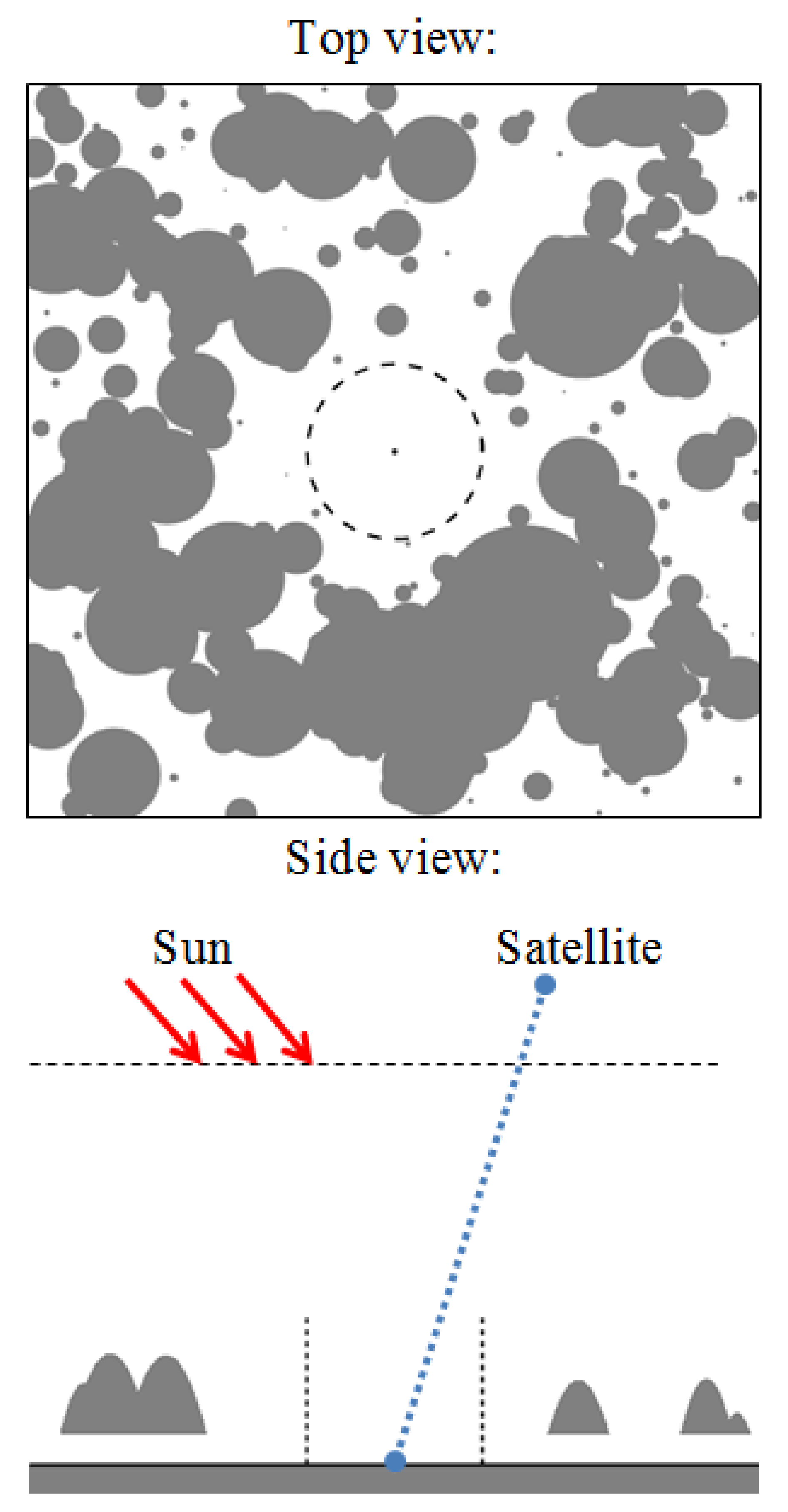
The problem is formulated as follows (
Figure 1).
Let there be the flat atmosphere—the ground surface system. The parallel solar radiation flux is incident on the upper boundary of the atmosphere at the angles
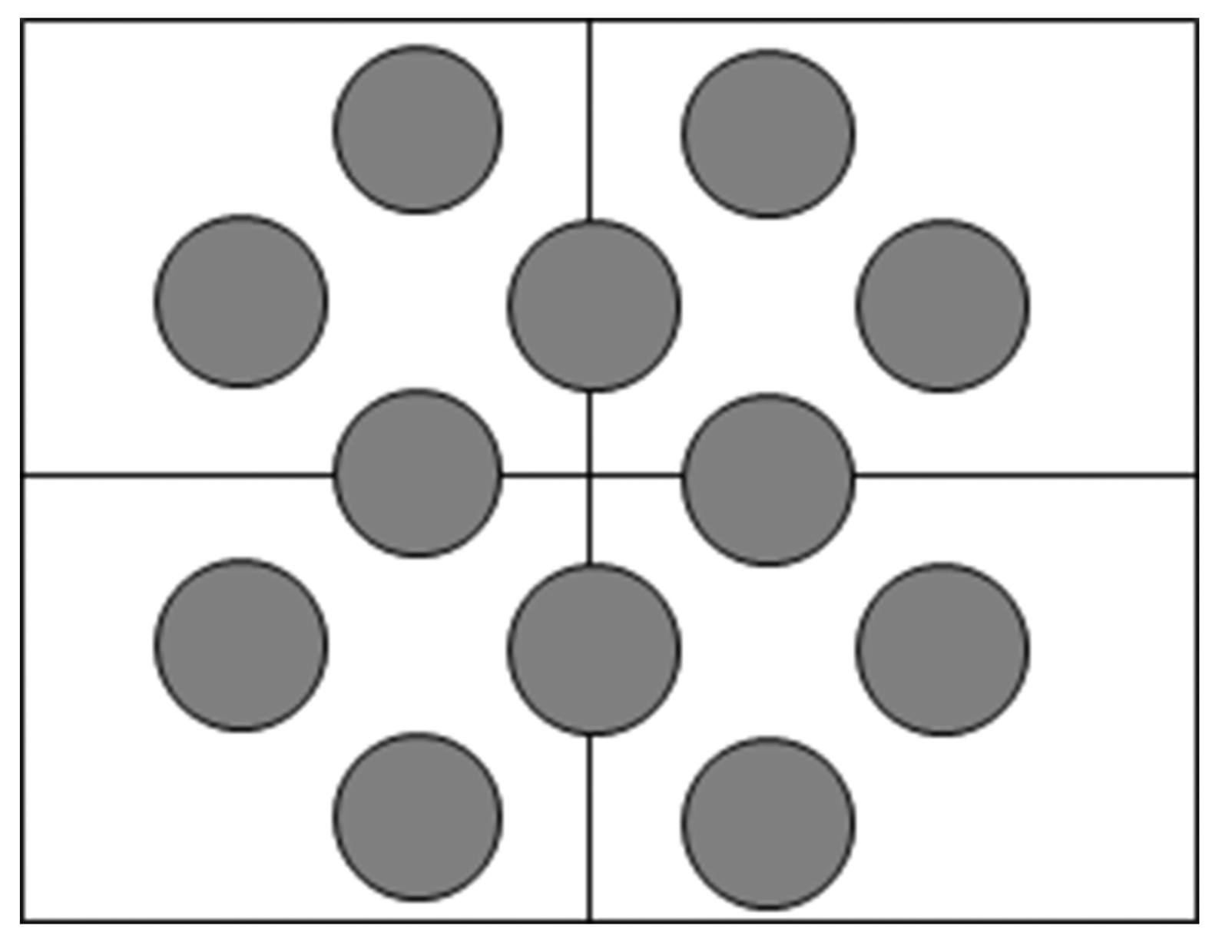
. Let the statistically homogeneous Poisson cloud field consist of paraboloids. The algorithm of constructing the Poisson fields of paraboloids described in [
13] was used for simulation. The number of clouds was random and obeyed the Poisson distribution with mathematical expectation presented in [
13] (pp. 119–125). The positions of cloud centers were random and uniformly distributed in the horizontal plane. The cloud shapes were similar, and their sizes were random and obeyed the exponential distribution [
13] (pp. 119–125) with the mathematical expectation equal to the average horizontal cloud size
. The deterministic cylindrical gap of radius
R was simulated within the cloud layer. The lower boundary of cloudiness was fixed and equal to
. The thickness of a separate cloud was random, but the average thickness was equal to
.
Let the cloud cover index be equal to
. The aerosol optical characteristics were homogeneous within the cloud medium and were determined by extinction and scattering coefficients and a scattering phase function. The optical model of cloudiness was constructed based on the OPAC cumulus cloud model [
20]. The optical characteristics of the cloudless atmosphere were described by the LOWTRAN-7 model [
21]. The homogeneous Lambert ground surface with the reflectance
was considered. The satellite sensing system was placed at the altitude
. Its optical axis was directed toward the point on the ground surface located in the center of the projection of the gap in the cloud field onto it. Radiation at the wavelength
was received at this point. The satellite zenith angle was
, and the azimuthal angle between the directions toward the receiver and the Sun from the observation point on the ground surface was equal to
.
It was necessary to estimate the gap radius for which the neglect of the cloud adjacency effect will introduce the error in the reconstructed reflectance less than 0.005 and will allow the mask of pixels to be constructed for which the reconstruction error will exceed 0.005.
The problem is solved in several steps:
- (1)
From the MODIS data, the cloudiness mask (MOD06L2 data), the AOD of cloudless areas (MOD04L2), the upper cloud boundaries (MOD06L2), the AOD of cloudiness (MOD06L2), the solar zenith angles , and the satellite zenith angle and the azimuth angle of the receiving system (MOD03L2) are determined.
- (2)
The AOD value averaged over clear sky pixels is determined.
- (3)
Among the LOWTRAN-7 cloudless models, the model is selected with the AOD value closest to that of the MODIS channel.
- (4)
From the MOD09L2 data, the average reflectance of cloudless areas is determined.
- (5)
From the AOD of cloudiness and the altitude of the upper cloud boundary , the cloud extinction coefficient is determined. The cloud medium is considered homogeneous. The quantum survival probability and the normalized cloud scattering phase function are selected from the LOWTRAN-7 models.
- (6)
The molecular scattering coefficient is selected from the mid-latitude summer LOWTRAN-7 models.
- (7)
The radiation intensities received by the satellite system and averaged over an ensemble of realizations of the cloud field for the examined optical and geometrical conditions, the preset average reflectance , are calculated by the Monte Carlo method depending on the gap radii R.
- (8)
The cloud adjacency effect on the reconstructed ground surface reflectance is estimated based on the expression for the total radiation intensity received by the satellite system in the cloudless case for the homogeneous ground surface (in the independent pixel approximation):
where
is the radiation intensity scattered in the atmosphere and not interacted with the ground surface for the cloudless atmosphere;
is the sun irradiance of the ground surface disregarding reflected radiation for the cloudless atmosphere;
is the atmospheric albedo (contribution of singly reflected radiation to the ground surface illumination in the cloudless atmosphere);
is the intensity of radiation reflected from the ground surface and recorded with the receiving system for the unit ground surface luminosity of the cloudless atmosphere.
From Formula (2), we obtain the expression for the reflectance
:
where
If we neglect the cloud adjacency effect at the point on the ground surface corresponding to the projection of the center in the gap of the cloudy field, we obtain the approximate value of the reflectance
:
where
is the total radiation received for satellite observations of the point on the ground surface located in the center of the deterministic gap with radius R.
Then, the gap radius
for which the neglect of the cloud adjacency effect introduces the reflectance reconstruction error
less than 0.005 is defined as the least radius
for which the condition
is satisfied.
- (9)
Proceeding from the radii , the mask of pixels is constructed for which the cloud adjacency effect is significant.
The radiation intensity
received by the satellite system and averaged over an ensemble of realizations of the cloud field was simulated by the backward Monte Carlo method [
22]. The trajectories were subdivided into
P packages, and each package comprised
N trajectories. The mean free path length beyond the cloud layer was simulated by the standard algorithm [
22] (p. 11). For the photon trajectories passing through the cloud layer
, the maximum cross-section method [
22] (p. 12) is widely used to simulate the mean free path length. However, our estimations have shown that the standard algorithm [
22] (p. 11) adapted by us for computations in a three-dimensional inhomogeneous medium is more economic from the viewpoint of the computational time. The scattering and absorption of photons in the medium was simulated by standard algorithms [
22] (p. 10). When a photon collided with the ground surface, its reflection was simulated, and its weight decreased by the probability of radiation absorption by the surface. At each collision point of the photon trajectory in the medium and collision with the ground surface, the local estimate of radiation coming at the upper boundary of the atmosphere in the direction toward the Sun was calculated from the formulas:
For the atmosphere
and for the ground surface
where
is the estimated intensity of radiation coming at the upper boundary of the atmosphere from the
kth collision point of the
nth trajectory from the
pth package;
is the energy (weight) of the photon at the collision point;
is the solar constant,
is the aerosol scattering coefficient,
is the molecular scattering coefficient, and
is the extinction coefficient at the collision point,
is the phase function of aerosol scattering at the angle
,
is the molecular scattering phase function, and
is the optical thickness of the layer from the collision point to the upper boundary of the atmosphere in the direction opposite to the direction of radiation incidence at the upper boundary of the atmosphere.
If the photon interacted with the medium within the cloud layer, the cloud optical aerosol characteristics were considered in Formulas (8) and (9), and if beyond the cloud layer, the aerosol characteristics of the cloudless layer were considered. It is difficult to calculate from Formulas (8) and (9), because the collision point can lie below, within, or above the cloud layer; the ray trajectory from the collision point toward the Sun can intersect the deterministic gap of the cloud field; and it also can intersect cloud boundaries or clouds can partially overlap each other.
Then, the total radiation intensity is calculated from the formula:
where
P is the number of trajectory packages,
N is the number of photon trajectories in one package (
trajectories altogether),
is the number of collisions for the
nth trajectory from the
pth package. The error of estimate (10) is calculated from the formula:
4. Interpolation Formula for Estimating
Using the developed program of the Monte Carlo method, we calculated values for five MODIS channels and a wide range of optical and geometrical conditions. Calculations were carried out for the following conditions:
5 MODIS channels ( = 0.41, 0.47, 0.55, 0.68, and 0.86 m);
Cloud layer thicknesses = 0.5, 1.5, 4, and 6 km;
Cloud cover indices = 0.05, 0.15, 0.3, and 0.5;
Solar zenith angles = 0, 30, 45, and 60;
Zenith angles of the receiving system = 0, 30, 45, and 60;
Azimuthal angle ;
Ground surface reflectances = 0, 0.1, 0.3, 0.5, and 1;
Midlatitude summer model;
Aerosol optical depth of the cloudless atmosphere = 0, 0.09, 0.3, and 0.89;
Cloud extinction coefficients = 10, 20, 30, and 40 km.
Calculations were carried out only for one azimuthal angle because our estimations showed that the cloud adjacency effect is maximal at = 0. Calculations were carried out for 102,400 computational grid nodes.
Based on the results of calculations, the program was developed that allowed the radius of the cloud adjacency effect to be estimated, obviating the necessity of simulation of radiation transfer in an atmospheric layer. The program is given in [
23]. In the program, generalization of bilinear interpolation over the seven-dimensional grid of values is used:
where
,
, ⋯,
are constants adjusted so that the interpolation formula yielded results coinciding in the computational grid nodes with the calculated ones;
is the AOD of the cloudless atmosphere for the corresponding channel.
To estimate the possibilities of the interpolation formula, two series of comparisons were performed for the following optical and geometrical conditions: (1)
= 0.41, 0.55, and 0.86
m,
= 0.09,
= 0–0.5,
= 1.5 km,
,
,
= 20 km
, and
= 0.1; (2)
= 0.41, 0.55, 0.86
m,
= 0.09,
= 0.3,
= 1.5 km,
,
,
= 20 km
, and
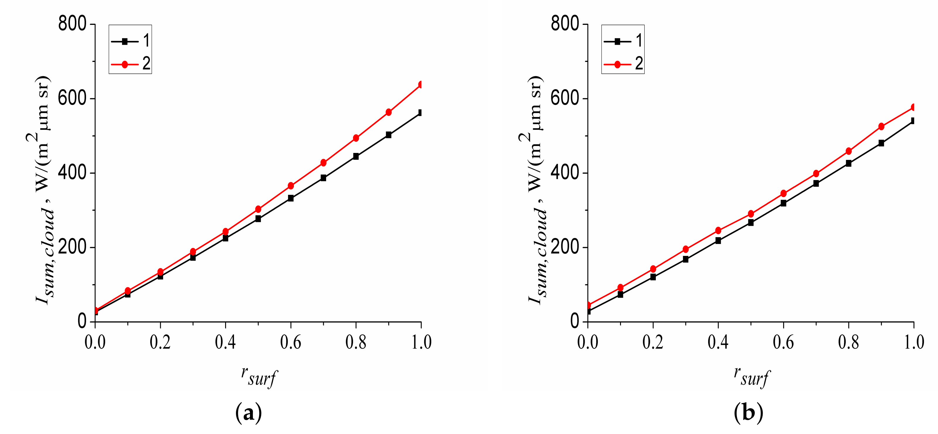
= 0–1. Results of comparison of the calculated and interpolated data are shown in
Figure 4. From
Figure 4, it can be seen that the calculated and interpolated data coincide at the nodal points. The average difference between the results of calculations and interpolations in
Figure 4a was
= 2.9 km at
= 0.41
m,
= 1.5 km at
= 0.55
m, and
= 0.4 km at
= 0.86
m. The average differences between the calculated and interpolated results shown in
Figure 4b was
= 0.4 km at
= 0.41
m,
= 0.1 km at
= 0.55
m, and
= 0.05 km at
= 0.86
m. The reason for the differences between the calculated and interpolated values at intermediate grid nodes is the following. The values of
,
,
,
, and
were calculated by the Monte Carlo method with a statistical error of less than 0.01%. However, for
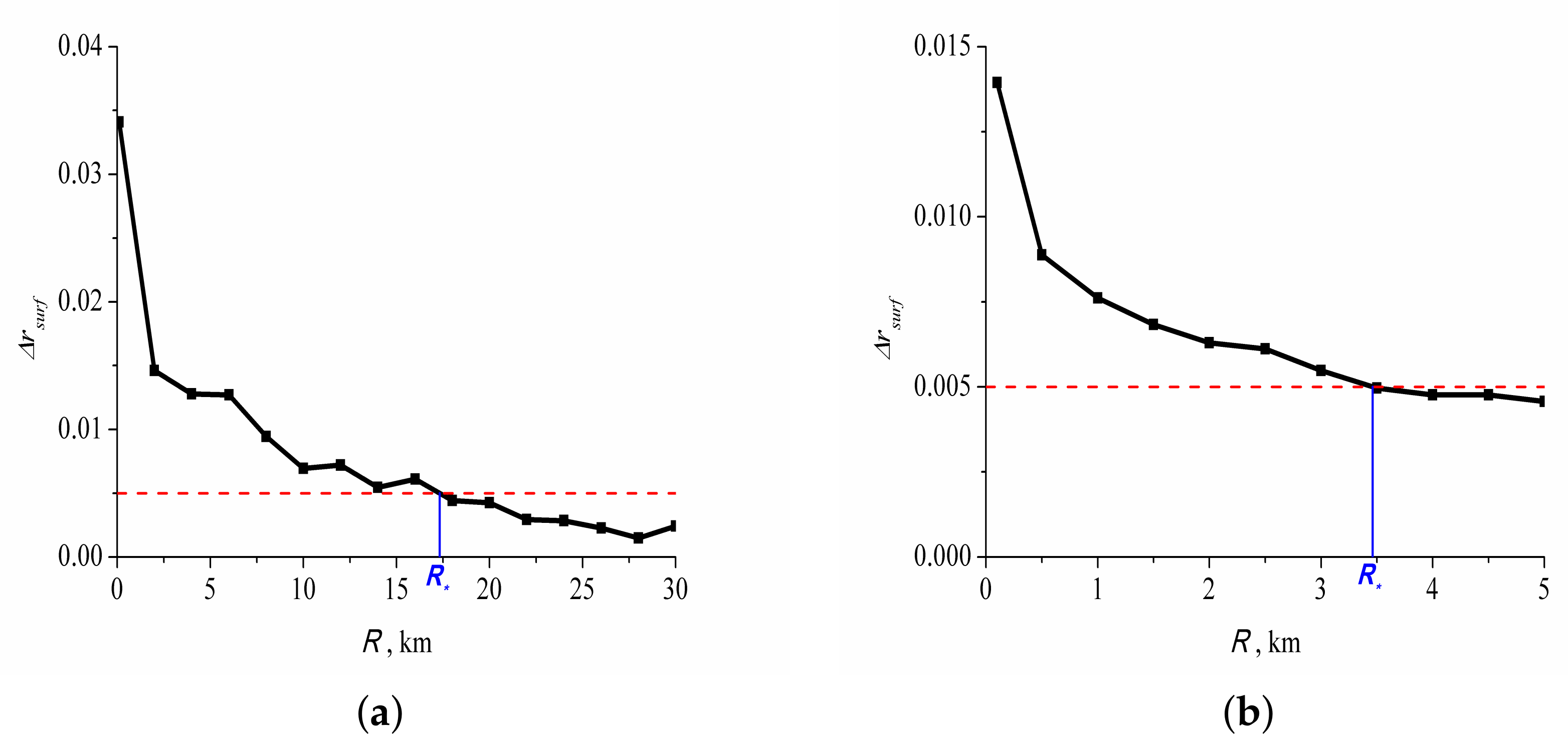
values close to 0.005, the derivative
is small; therefore, the computing error of the Monte Carlo method introduces a significant error in the definition of
. In particular, this error is the main reason for the observed discrepancy between the calculations and interpolation in
Figure 4. The special feature in the behavior of
is clearly shown in
Figure 5a. An analogous special feature in the behavior of
can also be seen in Figure 11 of the work [
6] for distances from the cloud greater than 2–3 km.
From
Figure 4b, it can be seen that with increasing
, the
values for some situations decrease, and for others increase. The reason is that, on the one hand, with increasing
, the relative contribution of
= 0.005 to the
value decreases, and on the other hand,
increases with
. On the whole, from
Figure 4, it can be seen that the proposed interpolation formula solves well the problem of determining the
value. The proposed approximation formula can be used for five MODIS channels (Nos. 1–4 and 8) under the following observation conditions: presence of cumulus cloudiness, cloud cover indices
from 0 to 0.5, ground surface reflectances
from 0 to 1, aerosol optical depths of the cloudless atmosphere
from 0 to 0.89, cloud extinction coefficients in the range from 10 to 40 km
, solar zenith angles and zenith angles of the receiving system from 0 to 60
, and azimuthal angle
from 0 to 180
. Calculations were carried out for cloudless midlatitude summer LOWTRAN-7 models. As shown by the preliminary estimates, the difference between the results obtained can reach 10–20% for different models of the cloudless atmosphere, but the same AOD. In future, we plan to expand the possibilities of the algorithm for a wider set of models of cloudiness and cloudless atmosphere.
5. Approbation Method
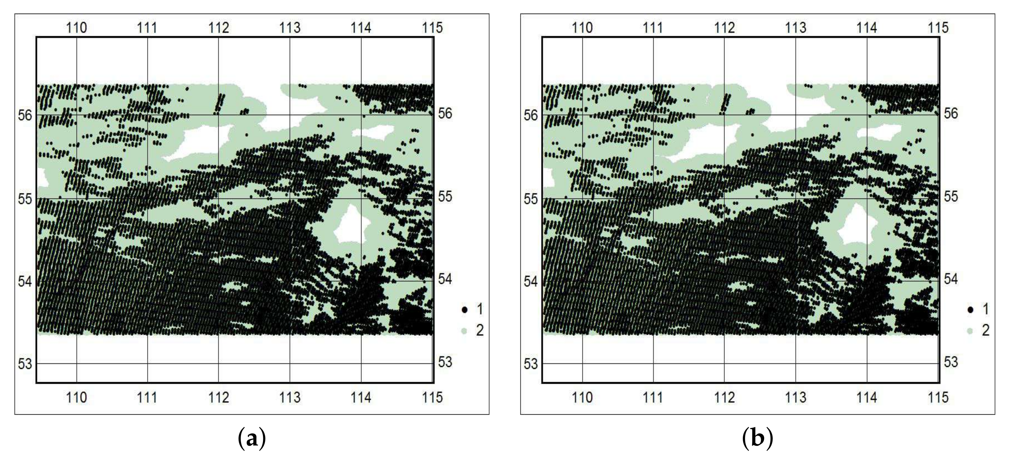
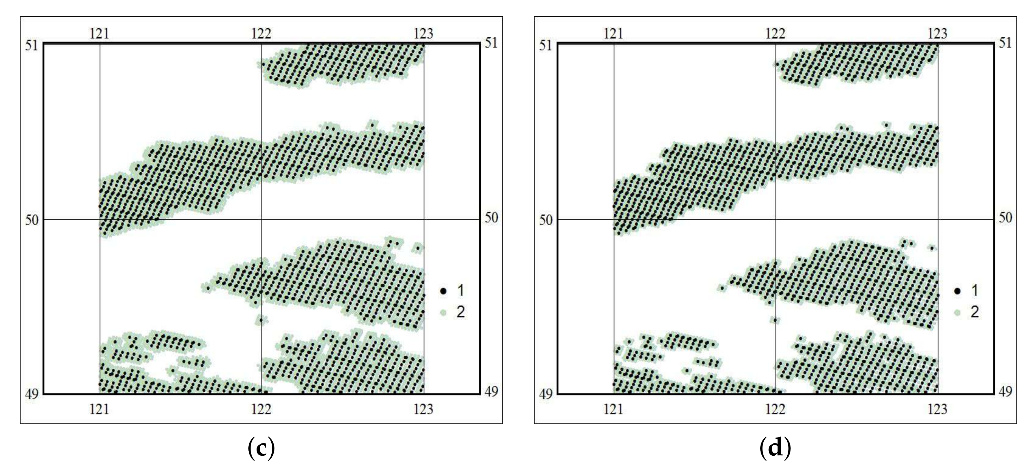
For approbation of the interpolation formulas, two fragments of the MODIS image MOD021KM.A2017172.0325.006.2017172133827.hdf recorded on June 21, 2017 were analyzed. These two fragments were chosen because the average AOD of cloudless areas was significant for the first fragment, whereas for the second fragment, it was much smaller. Calculations were carried out for the fourth MODIS channel (centered at
= 0.55
m). The average values used in calculations of the fragments and the fragment boundaries are presented in
Table 1. The average cloud size was
= 1 km, and the lower cloud boundary was at the altitude
= 1 km. In this case,
entering into Formula (6) was calculated for
P = 300 and
N = 5000. For all results obtained,
0.01.
The
values calculated from Formula (7) are shown in
Figure 5.
Based on the results shown in
Figure 5 and the interpolation formula (12), the
values were calculated. The results obtained are presented in
Table 2. The mask of pixels located at distances
and less from the boundaries of the cloud projections onto the ground surface is shown in
Figure 6. The comparison of the calculated and interpolated
values differed by 2 km for fragment 1 and by 1.5 km for fragment 2. Thus, the interpolation allows one to estimate the radius of the cloud adjacency effect. Moreover, the computational time for the interpolation was, on average, 750 times less than with the application of the Monte Carlo method. This allows one to use the proposed method for problem solving in real time.
6. Conclusions
In this work, the method of estimating the cloud adjacency effect on the accuracy of the reconstructed reflectance of the ground surface areas non-shadowed by clouds based on calculation of the cloud field intensity averaged over an ensemble of realizations in the center of the entrance pupil of the receiving system has been proposed. The approbation of the method for two test fragments of the MODIS image MOD021KM.A2017172.0325.006. 2017172133827.hdf recorded in the fourth MODIS channel shows that the proposed interpolation formula allows the radius of the adjacency effect to be estimated. The difference between the values of the gap radius calculated by the Monte Carlo method and obtained by interpolation did not exceed 2 km for these areas.
In this stage of investigations, the interpolation formula for has been constructed for the midlatitude summer LOWTRAN-7 model and the OPAC model of cumulus cloudiness. In future, we plan to expand the possibilities of the algorithm to include other optical models of the atmosphere and cloudiness. The reliability of the results is provided by the performed test comparisons and the use of the well-known models of the atmosphere and cloudiness.
Verification of the results of this method is planned in the next stage of our research. It is suggested to use the following approach. For verification, a series of three images of the same cloudless fragments of the ground surface will be selected. Two images should not contain cloudiness at distances less than 50 km from the examined area, and in the third image, the cloudiness should be observed near the examined area. Then, analyzing the differences between the reconstructed reflectances, the distance from the cloudiness can be determined, for which these differences would be less than 0.005.
The advantages of the proposed approach over existing methods are that it allows one to estimate the adjacency effect averaged over an ensemble of cloud field realizations (cloud arrangement) on the reconstructed reflectance of cloudless ground surface areas with preliminary consideration of a wide range of optical and geometrical conditions of observations. Consideration of the deterministic gap allows more realistic situations to be examined compared to homogeneous cloud fields without deterministic gaps. In contrast to the above-mentioned papers [
10,
11], the proposed approach has no restrictions on the ground surface reflectance.


