
Pseudo-Invariant Feature-Based Linear Regression Model (PIF-LRM): An Effective Normalization Method to Evaluate Urbanization Impacts on Land Surface Temperature Changes


Abstract
:1. Introduction
2. Study Area and Dataset
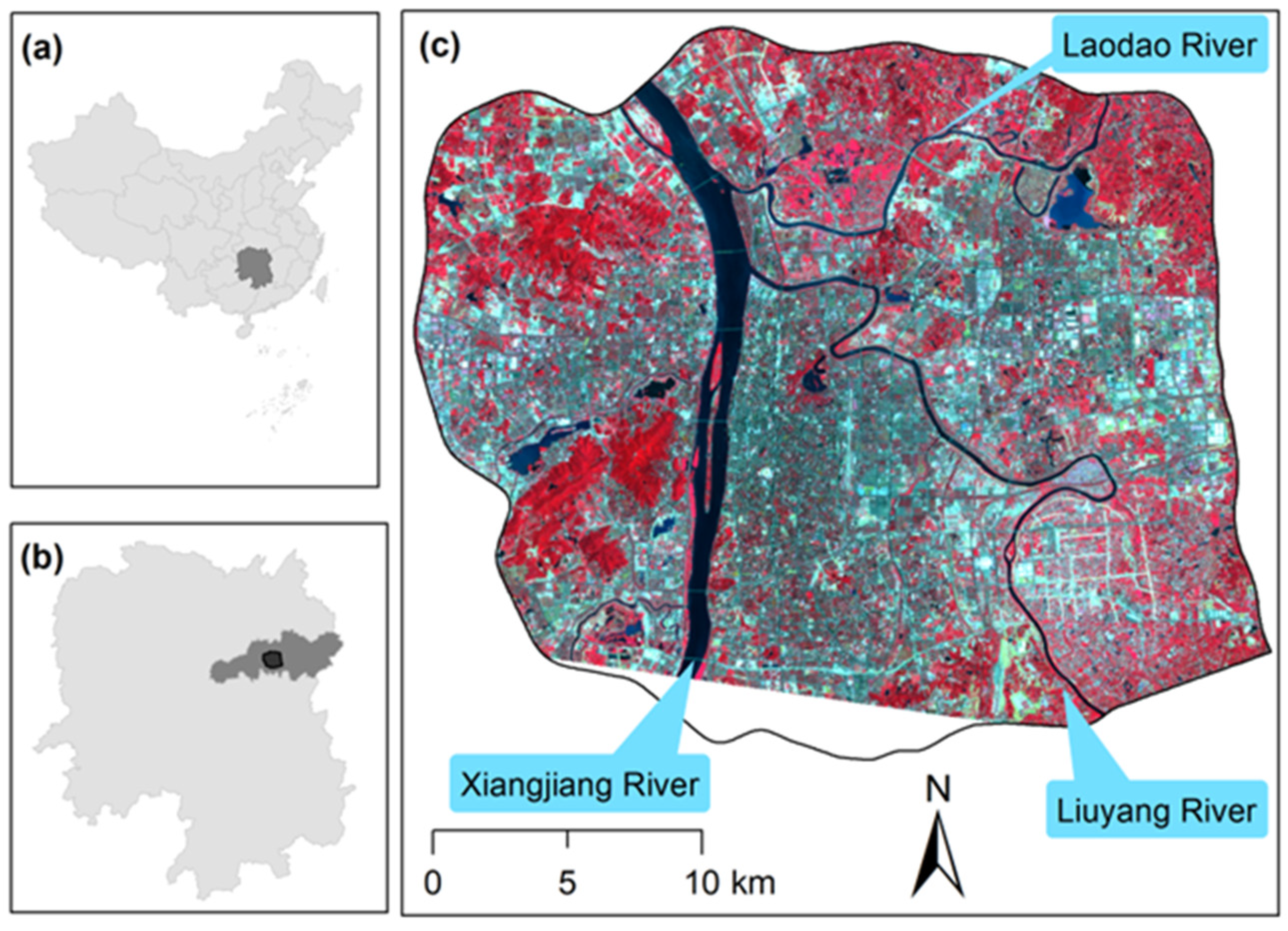
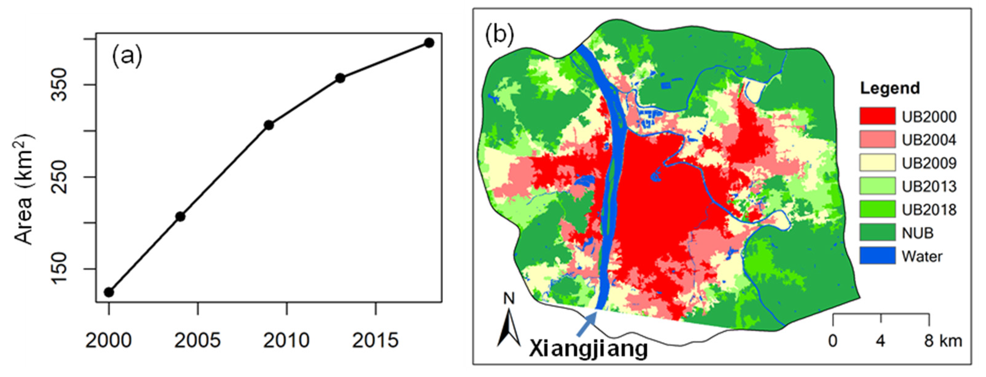
2.1. Study Area
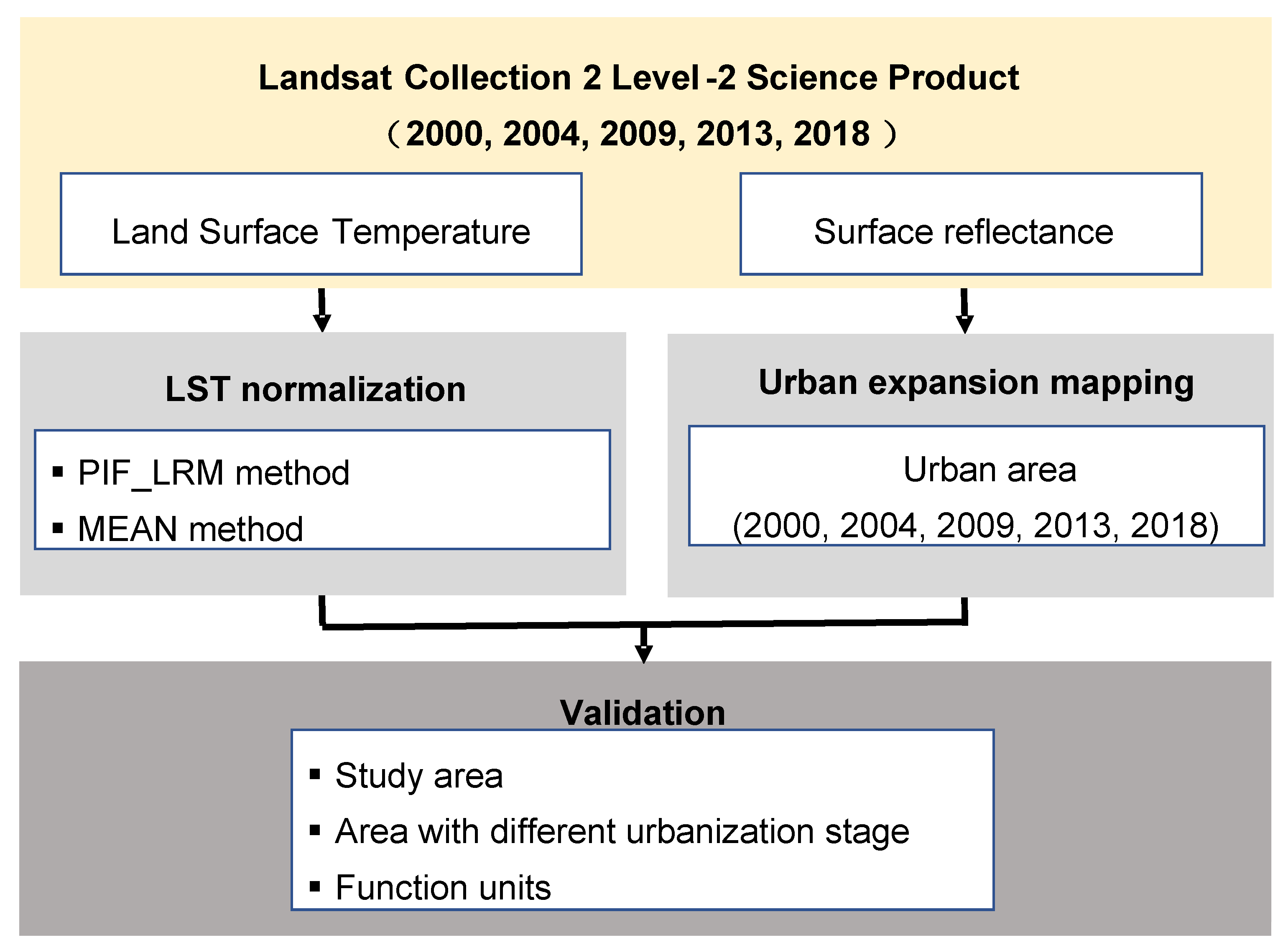
2.2. Dataset
3. Methods
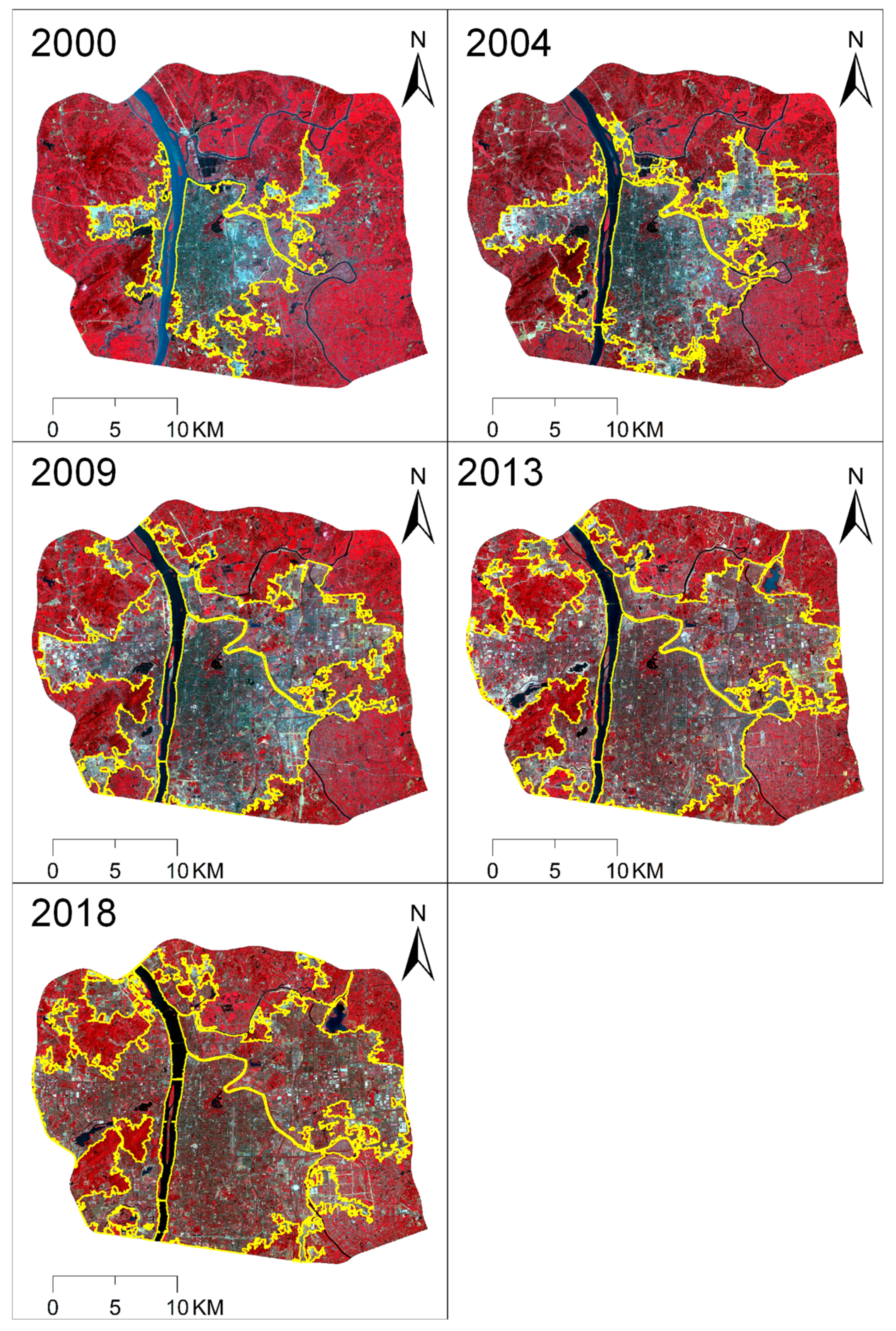
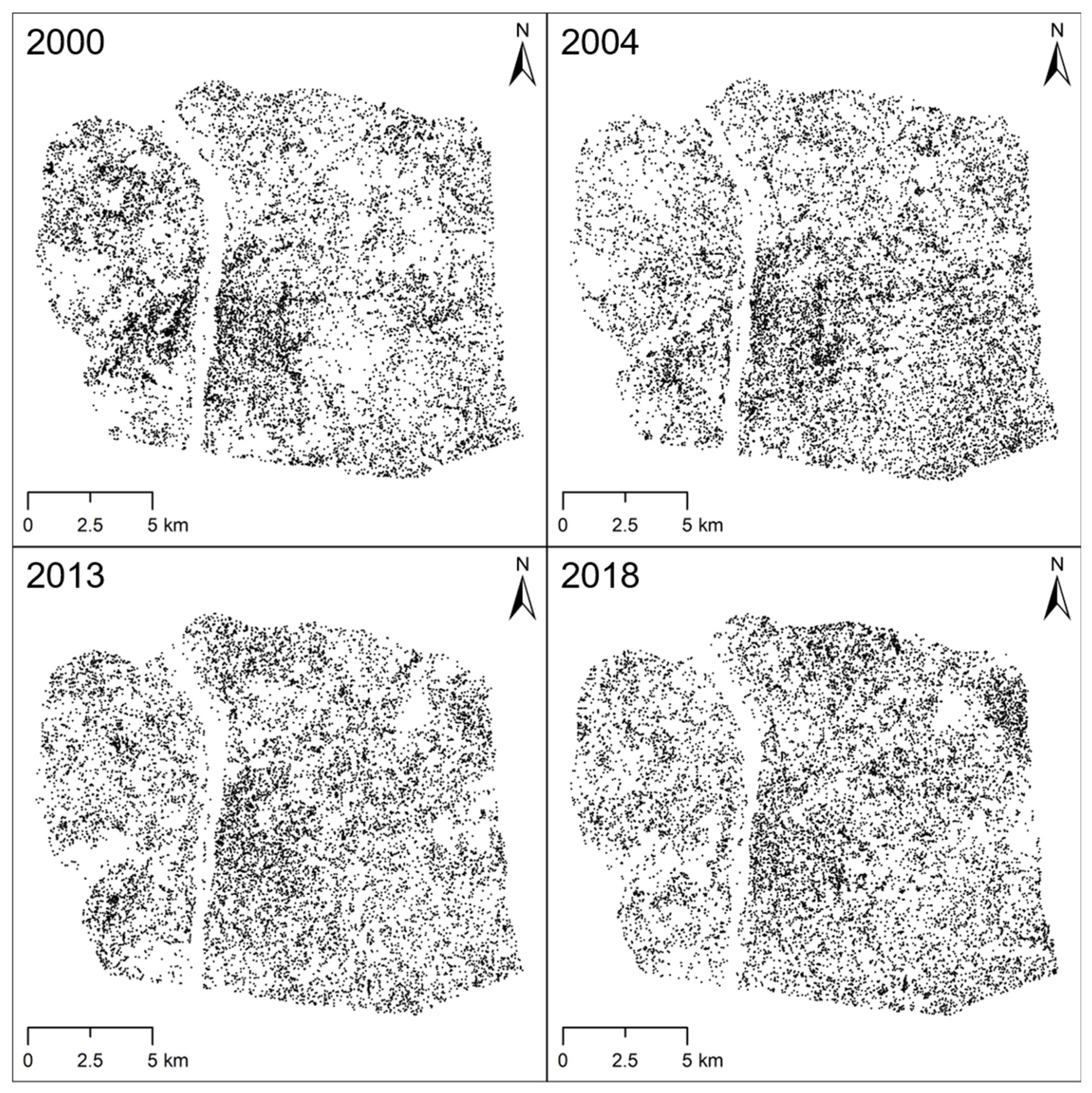
3.1. Mapping Urban Expansion
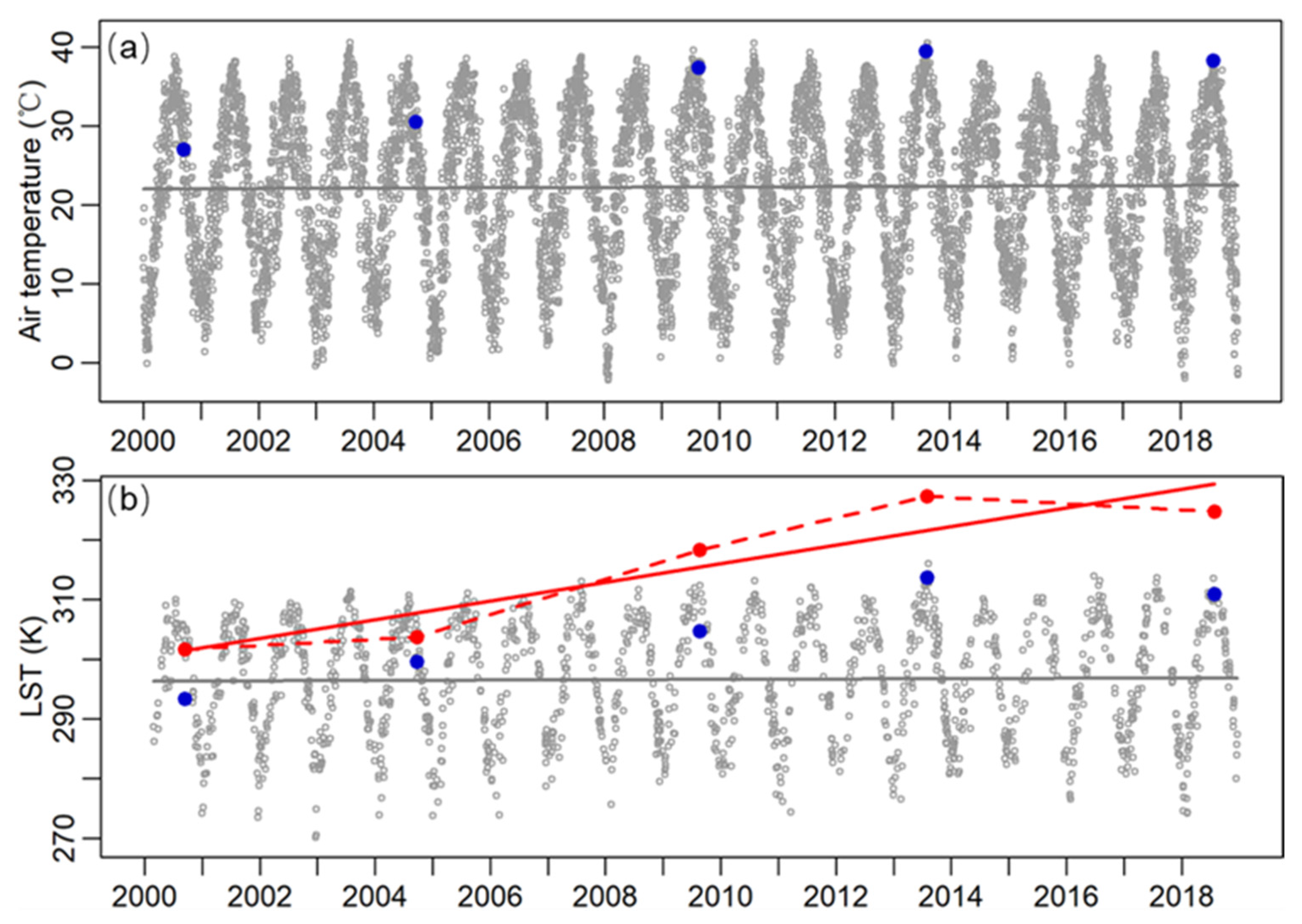
3.2. Normalizing LST Using PIF-LRM
3.3. Validation
4. Results
4.1. Urban Expansion
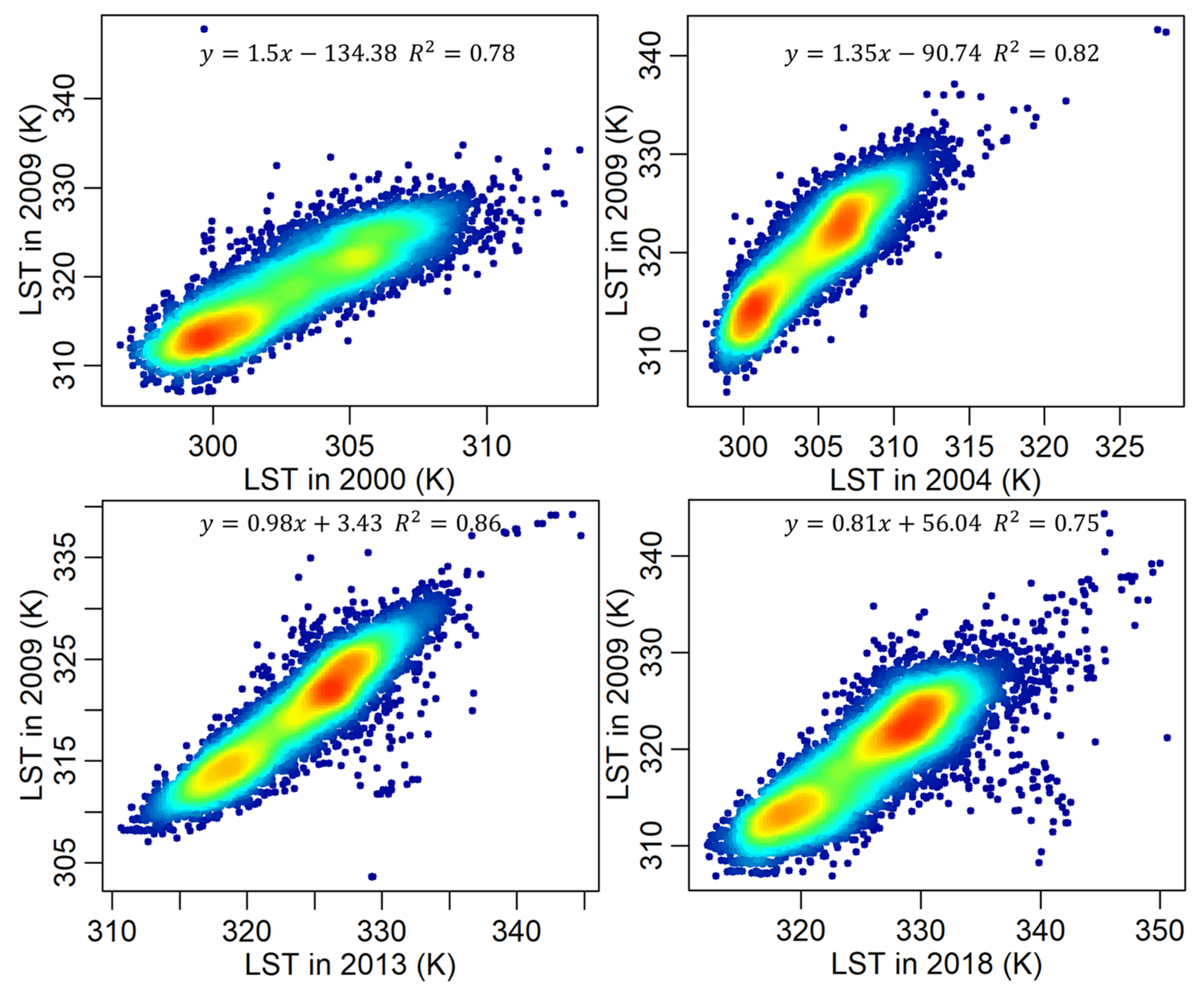
4.2. Statistical Relationship of the LST between the Reference and Target PIFs
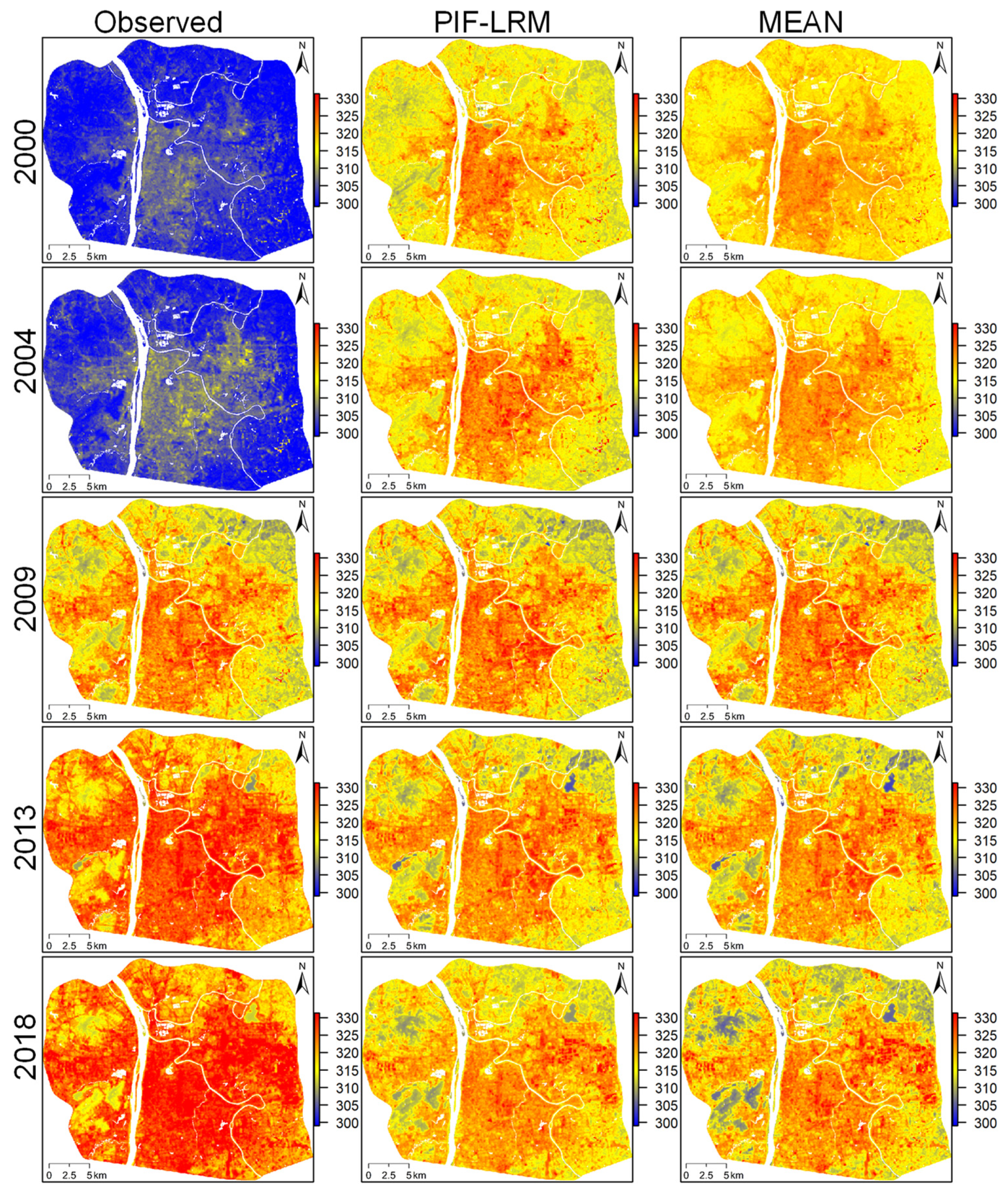
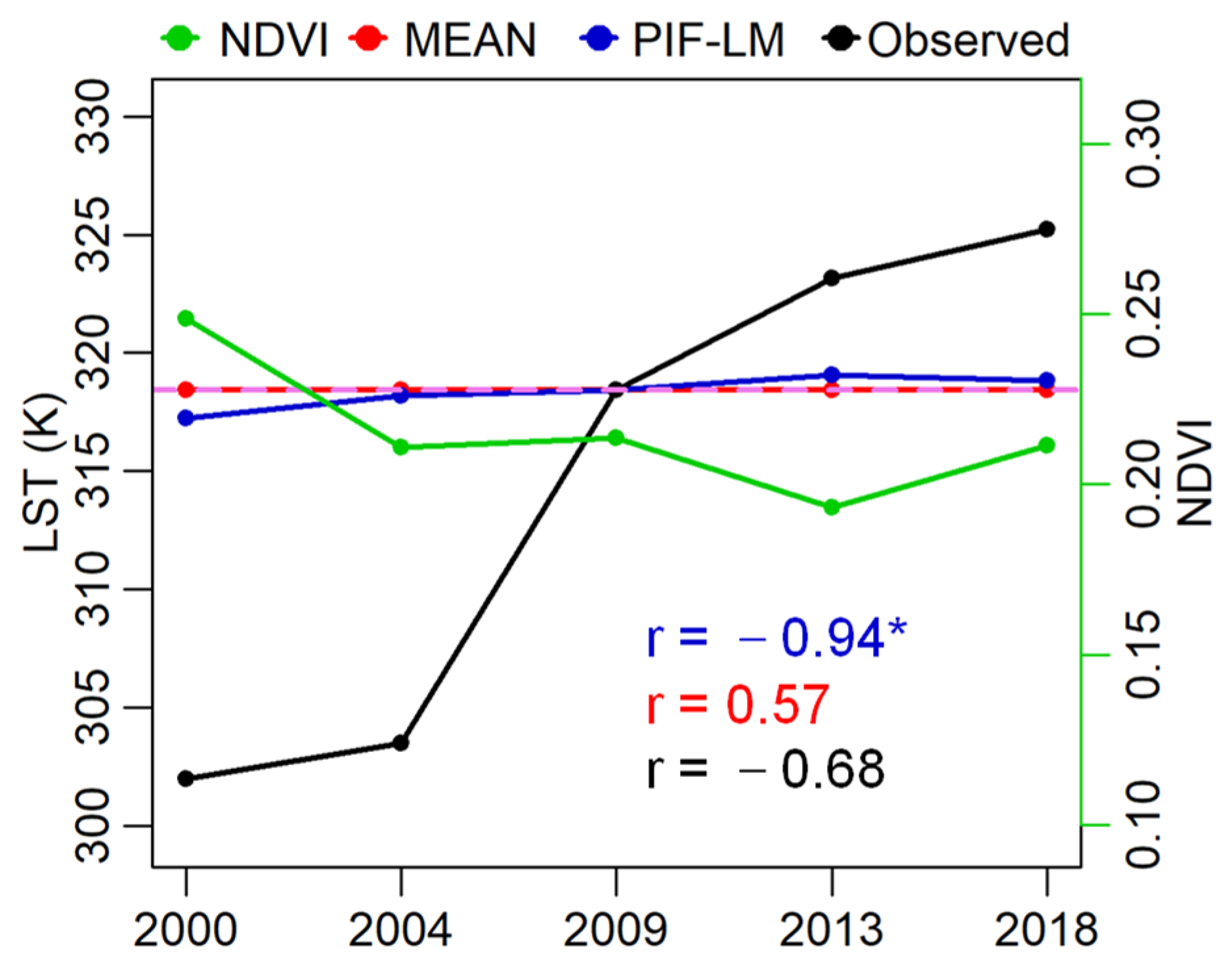
4.3. Validating the PIF-LRM at the Study Area Level
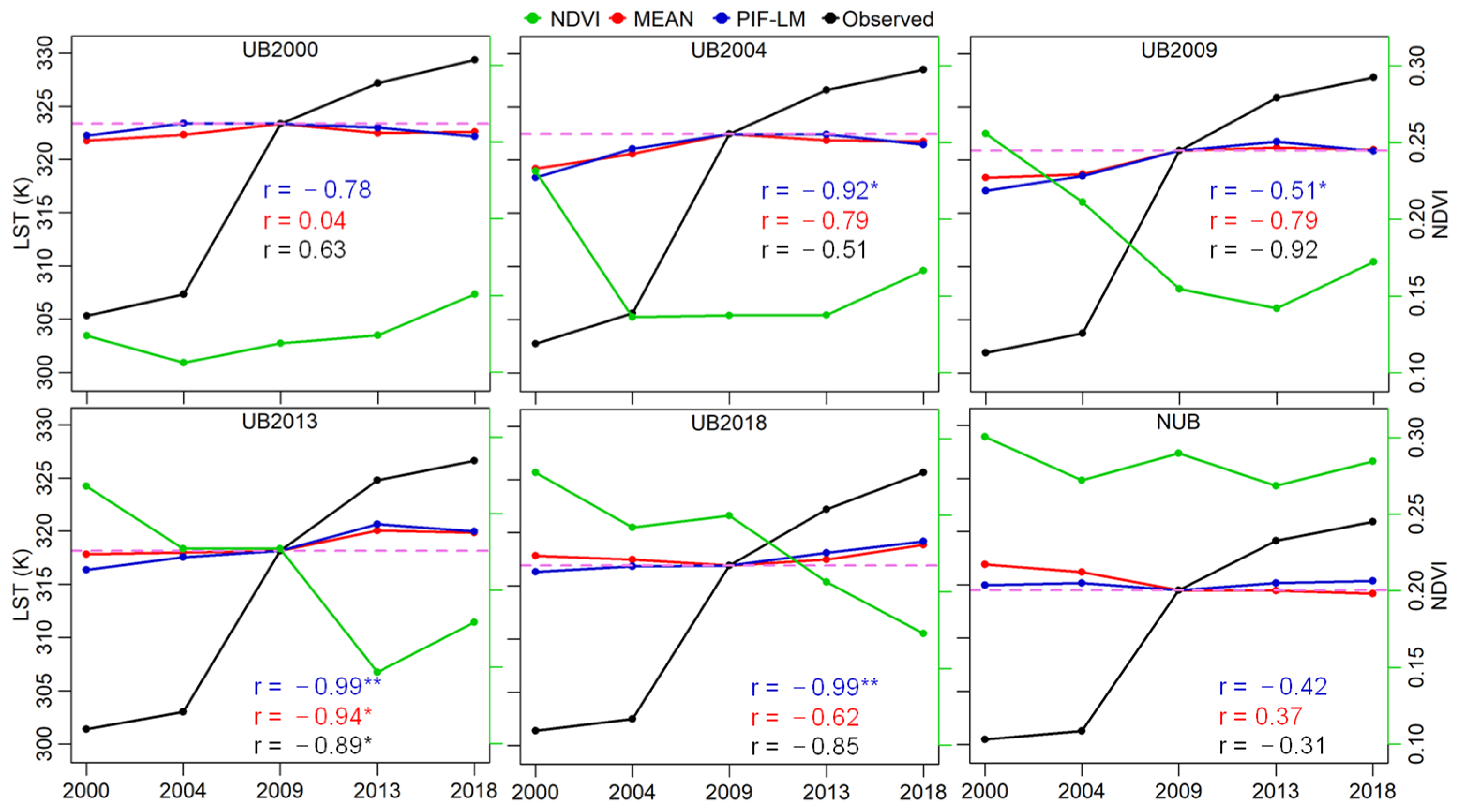
4.4. Validating PIF-LRM at the Zonal Level with Different Urbanization Stages
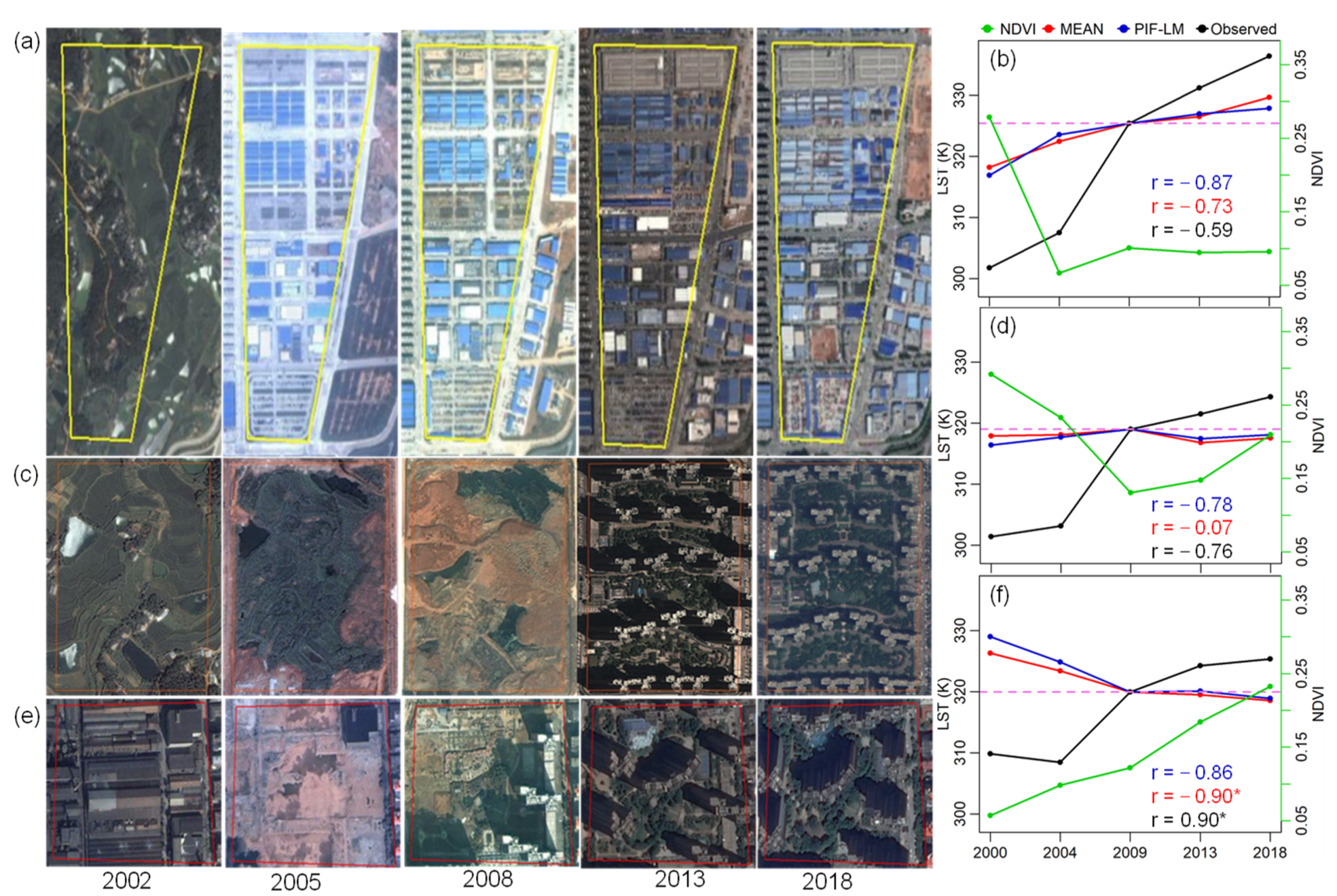
4.5. Validating PIF-LRM at the Local Level
5. Discussion
6. Conclusions
Supplementary Materials
Author Contributions
Funding
Institutional Review Board Statement
Informed Consent Statement
Data Availability Statement
Acknowledgments
Conflicts of Interest
References
- Meineke, E.; Youngsteadt, E.; Dunn, R.R.; Frank, S.D. Urban warming reduces aboveground carbon storage. Proc. R. Soc. B Biol. Sci. 2016, 283, 20161574. [Google Scholar] [CrossRef]
- Zhang, C.; Tian, H.; Pan, S.; Lockaby, G.; Chappelka, A. Multi-factor controls on terrestrial carbon dynamics in urbanised areas. Biogeosci. Discuss. 2014, 11, 17597–17631. [Google Scholar]
- Li, X.; Zhou, Y.; Yu, S.; Jia, G.; Li, H.; Li, W. Urban heat island impacts on building energy consumption: A review of approaches and findings. Energy 2019, 174, 407–419. [Google Scholar] [CrossRef]
- Azevedo, J.A.; Chapman, L.; Muller, C.L. Urban heat and residential electricity consumption: A preliminary study. Appl. Geogr. 2016, 70, 59–67. [Google Scholar] [CrossRef]
- Cao, Q.; Yu, D.; Georgescu, M.; Wu, J.; Wang, W. Impacts of future urban expansion on summer climate and heat-related human health in eastern china. Environ. Int. 2018, 112, 134–146. [Google Scholar] [CrossRef] [PubMed]
- Founda, D.; Santamouris, M. Synergies between urban heat island and heat waves in athens (greece), during an extremely hot summer (2012). Sci. Rep. 2017, 7, 10973. [Google Scholar] [CrossRef]
- Zhou, D.; Xiao, J.; Bonafoni, S.; Berger, C.; Deilami, K.; Zhou, Y.; Frolking, S.; Yao, R.; Qiao, Z.; Sobrino, J.A. Satellite remote sensing of surface urban heat islands: Progress, challenges, and perspectives. Remote Sens. 2018, 11, 48. [Google Scholar] [CrossRef]
- Waseem, S.; Khayyam, U. Loss of vegetative cover and increased land surface temperature: A case study of islamabad, pakistan. J. Clean. Prod. 2019, 234, 972–983. [Google Scholar] [CrossRef]
- Grigoraș, G.; Urițescu, B. Land use/land cover changes dynamics and their effects on surface urban heat island in bucharest, romania. Int. J. Appl. Earth Obs. Geoinf. 2019, 80, 115–126. [Google Scholar] [CrossRef]
- Peng, J.; Xie, P.; Liu, Y.; Ma, J. Urban thermal environment dynamics and associated landscape pattern factors: A case study in the beijing metropolitan region. Remote Sens. Environ. 2016, 173, 145–155. [Google Scholar] [CrossRef]
- Wang, J.; Huang, B.; Fu, D.; Atkinson, P.M.; Zhang, X. Response of urban heat island to future urban expansion over the beijing–tianjin–hebei metropolitan area. Appl. Geogr. 2016, 70, 26–36. [Google Scholar] [CrossRef]
- Zhou, W.; Wang, J.; Qian, Y.; Pickett, S.T.A.; Li, W.; Han, L. The rapid but “invisible” changes in urban greenspace: A comparative study of nine chinese cities. Sci. Total Environ. 2018, 627, 1572–1584. [Google Scholar] [CrossRef]
- Sun, R.; Chen, L.; Braat, L.C. Effects of green space dynamics on urban heat islands: Mitigation and diversification. Ecosyst. Serv. 2017, 23, 38–46. [Google Scholar] [CrossRef]
- Yu, Z.; Yao, Y.; Yang, G.; Wang, X.; Vejre, H. Spatiotemporal patterns and characteristics of remotely sensed region heat islands during the rapid urbanization (1995–2015) of southern china. Sci. Total Environ. 2019, 674, 242–254. [Google Scholar] [CrossRef]
- Peres, L.D.F.; Lucena, A.J.D.; Rotunno Filho, O.C.; França, J.R.D.A. The urban heat island in Rio de Janeiro, Brazil, in the last 30 years using remote sensing data. Int. J. Appl. Earth Obs. Geoinf. 2018, 64, 104–116. [Google Scholar] [CrossRef]
- Estoque, R.C.; Murayama, Y.; Myint, S.W. Effects of landscape composition and pattern on land surface temperature: An urban heat island study in the megacities of southeast asia. Sci. Total Environ. 2017, 577, 349–359. [Google Scholar] [CrossRef]
- Estoque, R.C.; Murayama, Y. Monitoring surface urban heat island formation in a tropical mountain city using landsat data (1987–2015). Isprs J. Photogramm. Remote Sens. 2017, 133, 18–29. [Google Scholar] [CrossRef]
- Masoudi, M.; Tan, P.Y.; Fadaei, M. The effects of land use on spatial pattern of urban green spaces and their cooling ability. Urban Clim. 2021, 35, 100743. [Google Scholar] [CrossRef]
- Zhang, H.; Li, T.-T.; Han, J.-J. Quantifying the relationship between land use features and intra-surface urban heat island effect: Study on downtown shanghai. Appl. Geogr. 2020, 125, 102305. [Google Scholar] [CrossRef]
- Dutta, I.; Das, A. Exploring the spatio-temporal pattern of regional heat island (rhi) in an urban agglomeration of secondary cities in eastern india. Urban Clim. 2020, 34, 100679. [Google Scholar] [CrossRef]
- Rahman, M.M.; Hay, G.J.; Couloigner, I.; Hemachandran, B.; Bailin, J. A comparison of four relative radiometric normalization (rrn) techniques for mosaicing h-res multi-temporal thermal infrared (tir) flight-lines of a complex urban scene. ISPRS J. Photogramm. Remote Sens. 2015, 106, 82–94. [Google Scholar] [CrossRef]
- Yue, W.; Qiu, S.; Xu, H.; Xu, L.; Zhang, L. Polycentric urban development and urban thermal environment: A case of hangzhou, china. Landsc. Urban Plan. 2019, 189, 58–70. [Google Scholar] [CrossRef]
- Schott, J.R.; Salvaggio, C.; Volchok, W.J. Radiometric scene normalization using pseudoinvariant features. Remote Sens. Environ. 1988, 26, 1–16. [Google Scholar] [CrossRef]
- Du, Y.; Teillet, P.M.; Cihlar, J. Radiometric normalization of multitemporal high-resolution satellite images with quality control for land cover change detection. Remote Sens. Environ. 2000, 82, 123–134. [Google Scholar] [CrossRef]
- Syariz, M.A.; Lin, B.-Y.; Denaro, L.G.; Jaelani, L.M.; Van Nguyen, M.; Lin, C.-H. Spectral-consistent relative radiometric normalization for multitemporal landsat 8 imagery. ISPRS J. Photogramm. Remote Sens. 2019, 147, 56–64. [Google Scholar] [CrossRef]
- Chen, X.; Vierling, L.; Deering, D. A simple and effective radiometric correction method to improve landscape change detection across sensors and across time. Remote Sens. Environ. 2005, 98, 63–79. [Google Scholar] [CrossRef]
- Wei, Y.; Liu, H.; Song, W.; Yu, B.; Xiu, C. Normalization of time series dmsp-ols nighttime light images for urban growth analysis with pseudo invariant features. Landsc. Urban Plan. 2014, 128, 1–13. [Google Scholar] [CrossRef]
- Rajasekar, U.; Weng, Q. Spatio-temporal modelling and analysis of urban heat islands by using landsat tm and etm+ imagery. Int. J. Remote Sens. 2009, 30, 3531–3548. [Google Scholar] [CrossRef]
- Hunan Daily. Urbanlization Level Increased from 20.5% to 77.6% in Changsha for the Past 40 Years (1978–2017). 2018. Available online: https://m.voc.com.cn/wxhn/article/201810/201810210851314915.html (accessed on 21 November 2021).
- Morning Hunan. Urban Heat Island in Changsha-Zhuzhou-Xiangtan in the Past 20 Years: Increased from 3 °C to 7 3 °C. 2016. Available online: http://www.xxcb.cn/event/hunan/2016-06-23/9059122.html (accessed on 21 November 2021).
- Li, C.; Li, J.; Wu, J. Quantifying the speed, growth modes, and landscape pattern changes of urbanization: A hierarchical patch dynamics approach. Landsc. Ecol. 2013, 28, 1875–1888. [Google Scholar] [CrossRef]
- Xu, H. Modification of normalised difference water index (ndwi) to enhance open water features in remotely sensed imagery. Int. J. Remote Sens. 2006, 27, 3025–3033. [Google Scholar] [CrossRef]
- Li, X.; Zhou, W. Optimizing urban greenspace spatial pattern to mitigate urban heat island effects: Extending understanding from local to the city scale. Urban For. Urban Green. 2019, 41, 255–263. [Google Scholar] [CrossRef]
- Zhou, D.; Zhao, S.; Liu, S.; Zhang, L.; Zhu, C. Surface urban heat island in china’s 32 major cities: Spatial patterns and drivers. Remote Sens. Environ. 2014, 152, 51–61. [Google Scholar] [CrossRef]
- Zhou, D.; Bonafoni, S.; Zhang, L.; Wang, R. Remote sensing of the urban heat island effect in a highly populated urban agglomeration area in east china. Sci. Total Environ. 2018, 628–629, 415–429. [Google Scholar] [CrossRef]
- Peng, J.; Ma, J.; Liu, Q.; Liu, Y.; Hu, Y.N.; Li, Y.; Yue, Y. Spatial-temporal change of land surface temperature across 285 cities in china: An urban-rural contrast perspective. Sci. Total Environ. 2018, 635, 487–497. [Google Scholar] [CrossRef]
- Halder, B.; Bandyopadhyay, J.; Banik, P. Monitoring the effect of urban development on urban heat island based on remote sensing and geo-spatial approach in kolkata and adjacent areas, india. Sustain. Cities Soc. 2021, 74, 103186. [Google Scholar] [CrossRef]
- Zhou, D.; Zhang, L.; Hao, L.; Sun, G.; Liu, Y.; Zhu, C. Spatiotemporal trends of urban heat island effect along the urban development intensity gradient in china. Sci. Total Environ. 2016, 544, 617–626. [Google Scholar] [CrossRef] [PubMed]
- Yao, R.; Wang, L.; Huang, X.; Zhang, W.; Li, J.; Niu, Z. Interannual variations in surface urban heat island intensity and associated drivers in china. J. Environ. Manag. 2018, 222, 86–94. [Google Scholar] [CrossRef]
- Xue, Y.; Lu, H.; Guan, Y.; Tian, P.; Yao, T. Impact of thermal condition on vegetation feedback under greening trend of china. Sci. Total Environ. 2021, 785, 147380. [Google Scholar] [CrossRef] [PubMed]


Publisher’s Note: MDPI stays neutral with regard to jurisdictional claims in published maps and institutional affiliations. |
© 2021 by the authors. Licensee MDPI, Basel, Switzerland. This article is an open access article distributed under the terms and conditions of the Creative Commons Attribution (CC BY) license (https://creativecommons.org/licenses/by/4.0/).
Share and Cite
Cai, Z.; Fan, C.; Chen, F.; Li, X. Pseudo-Invariant Feature-Based Linear Regression Model (PIF-LRM): An Effective Normalization Method to Evaluate Urbanization Impacts on Land Surface Temperature Changes. Atmosphere 2021, 12, 1540. https://0-doi-org.brum.beds.ac.uk/10.3390/atmos12111540
Cai Z, Fan C, Chen F, Li X. Pseudo-Invariant Feature-Based Linear Regression Model (PIF-LRM): An Effective Normalization Method to Evaluate Urbanization Impacts on Land Surface Temperature Changes. Atmosphere. 2021; 12(11):1540. https://0-doi-org.brum.beds.ac.uk/10.3390/atmos12111540
Chicago/Turabian StyleCai, Zhengwu, Chao Fan, Falin Chen, and Xiaoma Li. 2021. "Pseudo-Invariant Feature-Based Linear Regression Model (PIF-LRM): An Effective Normalization Method to Evaluate Urbanization Impacts on Land Surface Temperature Changes" Atmosphere 12, no. 11: 1540. https://0-doi-org.brum.beds.ac.uk/10.3390/atmos12111540