Sensitivity Operator Framework for Analyzing Heterogeneous Air Quality Monitoring Systems

Abstract

Air quality monitoring systems differ in composition and accuracy of observations and their temporal and spatial coverage. A monitoring system’s performance can be assessed by evaluating the accuracy of the emission sources identified by its data. In the considered inverse modeling approach, a source identification problem is transformed to a quasi-linear operator equation with the sensitivity operator. The sensitivity operator is composed of the sensitivity functions evaluated on the adjoint ensemble members. The members correspond to the measurement data element aggregates. Such ensemble construction allows working in a unified way with heterogeneous measurement data in a single-operator equation. The quasi-linear structure of the resulting operator equation allows both solving and predicting solutions of the inverse problem. Numerical experiments for the Baikal region scenario were carried out to compare different types of inverse problem solution accuracy estimates. In the considered scenario, the projection to the orthogonal complement of the sensitivity operator’s kernel allowed predicting the source identification results with the best accuracy compared to the other estimate types. Our contribution is the development and testing of a sensitivity-operator-based set of tools for analyzing heterogeneous air quality monitoring systems. We propose them for assessing and optimizing observational systems and experiments.

1. Introduction

Atmospheric air quality monitoring systems vary in their temporal and spatial coverage, the composition of the chemicals observed, and the accuracy of the data obtained. With the help of various monitoring systems, a huge amount of heterogeneous data is collected. The effective use of data is a significant scientific problem [1,2]. Moreover, new measurement systems are deployed to obtain new air-quality data, and new observational experiments are carried out. Choosing or optimizing the configuration of a monitoring system or observational experiment [3,4,5,6,7,8,9,10,11] is a multi-criteria decision-making task. It is necessary to compare the cost and accuracy of measuring equipment, maintenance costs, the goals of building such a system, its use cases, and other factors [12,13,14]. An essential criterion for choosing the configuration of the monitoring system is the value of the information content of prospective measurements. Hence, the methods of different accuracy and computational intensity for analyzing the information content of measurement data are essential. Finally, all the factors have to be compared, and a decision should be made about choosing the best variant. To choose one of the options, one can, for example, use the Multiple Criteria Decision-Making methods (see, e.g., [15]).

The joint use of process models and observational data makes it possible to solve a number of applied inverse problems, including the identification of air pollution sources and restoration of pollution fields in unobserved areas [3,4,16,17,18,19,20,21,22,23]. Data assimilation algorithms [24,25] are widely used in operative and quasi-operative air quality applications [26,27,28,29,30,31]. A data assimilation problem can be considered as the sequence of linked sources identification problems [32]. Air pollution sources pattern extracting is needed to compile emission inventories [33]. Knowing the emission sources is essential to model air quality since the emission sources largely determine the system’s behavior [34,35]. These considerations make the source identification problem’s solution accuracy a relevant instrument to measure the value of the information content of the observation data.

The methods of utilizing heterogeneous measurement data are referred to as “data fusion” [36,37,38]. Data of different sources and types can complement and cross-validate each other. In the paper, we focus on data fusion of heterogeneous measurements from the perspective of inverse modeling. In particular, previously, we considered the data obtained from the time series of concentrations at monitoring sites [39,40] and those were presented as images of concentration fields [41,42], as well as a combination of these two data types [43]. In the paper, we additionally consider Pointwise (in situ) monitoring data in space and time, which allows processing data from mobile monitoring systems mounted on ships [44], aircraft [45], unmanned aerial vehicles [46], and cars [47]. Moreover, the support for time-averaged concentration data is incorporated that allows one to include, for example, snow cover monitoring data, bio-monitoring techniques data, as well as the other, averaged data, for example, those published by Roshydromet [48].

Our approach is based on ensembles of solutions of adjoint equations and sensitivity operators. It consists of constructing families of sensitivity operators of various dimensions based on the inverse problems, linking the observed characteristics with the model’s uncertainty functions (e.g., emission sources). The approach bridges an idea proposed by G.I. Marchuk in [49], methods of sensitivity theory [50], the essence of the mollification method [51], and the “image to structure” operator concept [52]. In [49], G.I. Marchuk suggested gathering adjoint problem-based interpretations of separate measurement data elements to a single equation. In the case of many data elements (e.g., high-resolution satellite images), the straightforward application of the approach is complicated since one needs to solve a large number of adjoint problems, equal to the number of the considered data elements (e.g., pixels).

The first approach to this issue is considering a misfit cost function comparing the measured and simulated data. It dramatically decreases the ensemble of the adjoint problems to obtain the gradient of the cost function [53,54,55]. In this case, one has to solve only one adjoint problem, defined by the misfit between the measured and simulated data. This approach is widely used in the applications (see the review in [24,25]).

Another solution is to consider some arbitrary aggregates of the measurement data (which is relevant to the mollification method and the “image to structure” operator concept) and evaluate the set of adjoint problem solutions for these aggregates. The sensitivity operator is then composed of this adjoint problem solutions ensemble. Sensitivity operators allow formulating a family of quasi-linear operator equations for the inverse problem, the sets of solutions of which contain the solutions of the original problem. The quasi-linear structure of the equations provides a more straightforward way of analysis with the linear tools [39,41], compared to the case of the misfit cost function-based aggregation of the measurement data, i.e., the sensitivity operators can be used to solve and analyze the inverse problems in a unified way. Similar algorithms have been applied to the linear passive transport problem [56] and the nonlinear transport–transformation model with Pointwise sources and in situ measurements [20]. An overview of the other adjoint-ensemble-based methods can be found in [23].

Furthermore, the sensitivity of the operator-based approach allows naturally fusing various data types [57]. To do this, it is enough to construct the sensitivity operator from the adjoint problem solution ensembles corresponding to multiple data types (see Section 2.3 for more details).

The paper’s objective is to briefly describe the features of the proposed approach to solving inverse modeling problems using heterogeneous data coming from various monitoring systems. In particular, we want to study the characteristics of the sensitivity operator that can be used to predict the source identification results based on different monitoring system configurations. The ultimate goal of the study is to find a few characteristics that can be used in the observation system optimization that includes various data sources. The purpose of such optimization in the context of source identification is to reduce the source identification error by configuring the observation network. We can solve the corresponding inverse problems for different observation system configurations to measure this error, but their solution may take significant time. That is why we are looking for approximate estimates that are computationally cheaper.

The approach is tested on the air quality inverse modeling scenario for the domain containing the Baikal Natural Territory (BNT) (Figure 1). In 1996, UNESCO recognized Lake Baikal as a World Heritage Site [58]. In 1999, the Federal Law on the protection of Lake Baikal was adopted, which defined the concept of BNT, where environmental zoning was carried out, prescribing special conditions for implementing economic activities in each zone [59]. The Baikal region is located in Eastern Siberia in the belt of temperate latitudes, considerably far away from the oceans. However, the big water masses of about 23,000 km${}^3$ of fresh lake’s water leave their mark on the climate and weather in the region. The complex terrain, including high mountain ranges that frame the lake, contributes to the emergence of strong local winds, which even have unique names: Barguzin, Shelonik, Gornaya, etc. The region is exposed to various anthropogenic and natural factors. For example, it suffers from forest fires of different origins [60,61,62,63]. The industrial activity that develops in the region, mainly near urban settlements, certainly affects the quality of the environment [64,65,66].

This unique natural object, BNT, is observed by various means [44,63,67,68,69,70,71]. Hence, adequate measurement data-fusion is essential to carry out multidisciplinary studies in the region and provide the governing authorities with the necessary data to make decisions in terms of environmental protection to ensure the region’s sustainable development.

The paper is organized as follows: In Section 2.1, we state the basic source identification problem. Section 2.2 presents our sensitivity-operator-based framework. The supported measurement types are indicated in Section 2.3. Some approaches to analyze the measurement system data are considered in Section 2.4. Section 2.5 describes the inverse modeling scenario for BNT. In Section 3, we analyze the numerical results and discuss the conclusions in Section 4.

2. Materials and Methods

2.1. Chemical Transport Model

The Chemical Transport Model (CTM) for $l=1,\dots ,N_c$ reacting substances is considered in a domain ${\Omega }_T=\Omega \times (0,T)$, where $\Omega$ is a sufficiently smooth approximation of a bounded rectangular domain $[0,X]\times [0,Y]$ in ${\mathbb{R}}^2$, $T>0$. The domain ${\Omega }_T$ is bounded by $\partial {\Omega }_T=\partial \Omega \times [0,T]$.

$$\begin{array}{c}\frac{\partial {\phi }_l}{\partial t}-\nabla ·\left(\mathrm{diag}\left({\mu }_l\right)\nabla {\phi }_l-\mathbf{u}{\phi }_l\right)+P_l(t,\mathbf{\phi }){\phi }_l={\Pi }_l(t,\mathbf{\phi })+f_l+r_l,(\mathbf{x},t)\in {\Omega }_T,\end{array}$$

(1)

$$\begin{array}{c}\mathbf{n}·\left(\mathrm{diag}\left({\mu }_l\right)\nabla {\phi }_l\right)+{\beta }_l{\phi }_l={\alpha }_l,(\mathbf{x},t)\in {\Gamma }^{\left(out\right)}\subset \partial \Omega \times [0,T],\end{array}$$

(2)

$$\begin{array}{c}{\phi }_l={\alpha }_l,(\mathbf{x},t)\in {\Gamma }^{\left(in\right)}\subset \partial \Omega \times [0,T],\end{array}$$

(3)

$$\begin{array}{c}{\phi }_l={\phi }_l^0,\mathbf{x}\in \Omega ,t=0,\end{array}$$

(4)

where t is time and $\mathbf{x}$ is space coordinate, $N_c$ is the number of considered substances, ${\phi }_l={\phi }_l(\mathbf{x},t)$ denotes the concentration of the $l^{th}$ substance at a point $(\mathbf{x},t)\in {\Omega }_T$, $\mathbf{\phi }$ is the vector of ${\phi }_l(\mathbf{x},t)$ for $l=1,\dots ,N_c$, which is called the state function, and $L=\{1,\dots ,N_c\}$. The functions ${\mu }_l(\mathbf{x},t)\in {\mathbb{R}}^2$ correspond to the diffusion coefficients, $\mathrm{diag}\left(\mathbf{a}\right)$ is the diagonal matrix with the vector $\mathbf{a}$ on the diagonal, $\mathbf{u}(\mathbf{x},t)\in {\mathbb{R}}^2$ is the underlying wind speed. ${\Gamma }^{\left(in\right)}$ and ${\Gamma }^{\left(out\right)}$ are parts of domain boundary $\partial {\Omega }_T$ in which the vector $\mathbf{u}(\mathbf{x},t)$ points inwards the domain ${\Omega }_T$ and is zero or points outwards the domain ${\Omega }_T$, respectively, $\mathbf{n}$ is the outer normal. The functions ${\alpha }_l(\mathbf{x},t)$ and ${\phi }_l^0\left(\mathbf{x}\right)$ describe the boundary and initial conditions, respectively, ${\beta }_l$ is the boundary condition parameter, $f_l(\mathbf{x},t)$ is the a priori known source function. The transformation model defines loss and production operator elements $P_l,{\Pi }_l:[0,T]\times {\mathbb{R}}_{+}^{N_c}\to {\mathbb{R}}_{+}$. In the considered case of the chemical transformations, they are polynomials with positive time-dependent coefficients.

In our approach to inverse modeling, the model parameters are divided into “predefined parameters” $\mathbf{v}$ and “uncertainty functions” $\mathbf{q}$, belonging to some set Q. Most often, the uncertainty functions in the air quality studies are unknown sources of pollution $\mathbf{q}=\mathbf{r}$. To connect the current work with the other papers of the series, we intentionally keep a more complicated notation than it is needed to describe the considered problem. The presented approach is general and can be used as a framework for a broad spectrum of different inverse modeling problems. Let $\mathbf{r}\in Q$, where Q is the set of admissible sources, defined by a priori information:

• We suppose that only a given set of species $L_{src}$ is emitted. For the rest of species $r_l(\mathbf{x},t)=0$, $l\notin L_{src}$.
• The emission sources are supposed to be constant in time ($r_l(\mathbf{x},t)=r_l\left(\mathbf{x}\right)$).
• We do not require the emission sources to be positive since variables unconsidered in the model, chemical transformations, various land types, and meteorological conditions, such as rains and snowfalls, can act as sinks for the specific chemicals.

The rest of the parameters are considered as predefined, hence $\mathbf{v}=\left\{\mu ,\mathbf{u},\mathbf{\alpha },\mathbf{\beta },{\mathbf{\phi }}^0,\mathit{f}\right\}$. Let us define the pair of “direct” and “inverse” problems:

• In the Direct problem, $\mathbf{v}$ and $\mathbf{q}\in Q$ are given, and we find $\mathbf{\phi }$ from (1)–(4). The solution of the direct problem is denoted by $\mathbf{\phi }\left[\mathbf{q}\right]$. Let there be an “exact” uncertainty function value ${\mathbf{q}}^{(*)}={\mathbf{r}}^{(*)}$ to be found and ${\mathbf{\phi }}^{(*)}=\phi \left[{\mathbf{q}}^{(*)}\right]$ be the corresponding solution of the direct problem with the source function ${\mathbf{r}}^{(*)}$.
• In the Inverse problem, the uncertainty function ${\mathbf{q}}^{(*)}$ has to be identified from the partial information (“measurement data”) about ${\mathbf{\phi }}^{(*)}$, described in Section 2.3.

2.2. Sensitivity-Operator Based Representation of Measurement Data

We use the algorithm based on the sensitivity operators described in [39,41] to solve the source identification problem. It is based on the sensitivity relation, which links the model state function variation with that of the uncertainty function. For any ${\mathbf{q}}^{\left(2\right)},{\mathbf{q}}^{\left(1\right)}\in Q$:

$${〈S[{\mathbf{q}}^{\left(2\right)},{\mathbf{q}}^{\left(1\right)};h],{\mathbf{q}}^{\left(2\right)}-{\mathbf{q}}^{\left(1\right)}〉}_Q={〈h,\delta \phi 〉}_H.$$

(5)

Here $S[{\mathbf{q}}^{\left(2\right)},{\mathbf{q}}^{\left(1\right)};h]$ denotes the sensitivity function, which is calculated by the solution of the adjoint problem (the details can be found in [41]). The solution of the adjoint problem is determined by its source function h, which is defined by the measurement operator (see Section 2.3). Scalar products in (5) are:

$${〈a,b〉}_H=\sum _{l=1}^{N_c}{\int }_0^T{\int }_{\Omega }{a}_l(\mathbf{x},t)b_l(\mathbf{x},t)d\mathbf{x}dt,{〈a,b〉}_Q=\sum _{l=1}^{N_c}{\int }_{\Omega }{a}_l\left(\mathbf{x}\right)b_l\left(\mathbf{x}\right)d\mathbf{x}.$$

(6)

The right-hand side corresponds to an element of the measurement data.

If we consider a set of functions $U={\left\{h^{\left(\xi \right)}\right\}}_{\xi =1}^{\Xi }$, then combining the corresponding relations (5), we obtain a sensitivity operator relation

$$M_U\left[{\mathbf{q}}^{\left(2\right)},{\mathbf{q}}^{\left(1\right)}\right]\left({\mathbf{q}}^{\left(2\right)}-{\mathbf{q}}^{\left(1\right)}\right)=H_U\mathbf{\phi }\left[{\mathbf{q}}^{\left(2\right)}\right]-H_U\mathbf{\phi }\left[{\mathbf{q}}^{\left(1\right)}\right],$$

(7)

where

$$M_U\left[{\mathbf{q}}^{\left(2\right)},{\mathbf{q}}^{\left(1\right)}\right]z=\sum _{\xi =1}^{\Xi }{\mathbf{e}}^{\left(\xi \right)}{〈S[{\mathbf{q}}^{\left(2\right)},{\mathbf{q}}^{\left(1\right)};h^{\left(\xi \right)}],z〉}_Q,H_U\mathbf{\phi }=\sum _{\xi =1}^{\Xi }{\mathbf{e}}^{\left(\xi \right)}{〈h^{\left(\xi \right)},\mathbf{\phi }〉}_H.$$

Here ${\mathbf{e}}^{\left(\xi \right)}$ is the $\xi$-th element of the canonical basis in ${\mathbb{R}}^{\Xi }$. The adjoint functions corresponding to different elements of U, needed to compose the sensitivity operator, can be evaluated in parallel as an ensemble. Combining the ensembles of solutions of adjoint equations corresponding to different measurement data types into one sensitivity operator allows us to consider heterogeneous data.

If ${\mathbf{q}}^{(*)}$ is the exact solution of the source identification problem, I is the measurement data, aggregated in the state-function form (i.e., it is equal to ${\phi }^{(*)}$ in the parts of ${\Omega }_T$ where there are measurements and is zero otherwise), and $\delta I$ is its perturbation (i.e., the measurement noise), then for any U and $\mathbf{q}$ the relation holds:

$$M_U\left[{\mathbf{q}}^{(*)},\mathbf{q}\right]\left({\mathbf{q}}^{(*)}-\mathbf{q}\right)=H_{U}I+H_U\delta I-H_U\mathbf{\phi }\left[\mathbf{q}\right].$$

(8)

Quasi-linear operator Equation (8) can be solved by any appropriate operator equation solution method. In our work, we use the Newton–Kantorovich-type algorithm regularized with the truncated singular value decomposition (SVD) analogous to the algorithms in [41,42]. We present the algorithm in Appendix A. In this modification, we enforce the monotonic decrease of the discrepancy function with the iterations by choosing the appropriate step sizes.

2.3. Measurement Data Types

To use the approach, we have to present the measurement data in the form of a scalar product of the model state function with some projection functions. To define the measurements and corresponding projection functions h, we need appropriate delta-functions over space, time, and species denoted by $\delta$ and elements of the cosine-basis on the interval $[0,X]$:

$$C(X,\theta ,x)=\frac{1}{\sqrt{X}}\left\{\genfrac{}{}{0.0pt}{}{\sqrt{2}cos\left(\frac{\pi \theta x}{X}\right),\theta >0}{1,\theta =0}\right..$$

The elements of cosine-basis are used to transform image-type data to a finite set of values through Fourier transform. The symbol ${(.)}_{meas}$ denotes the parts of the domain where there are measurements available. For example, usually, only a small set $L_{meas}\subset \left\{1,\dots N_c\right\}$ of chemical species is monitored.

We consider the following measurement types defined by their correspondence to the model state function and projection functions $h^{\left(\xi \right)}$ in the sense of (6):

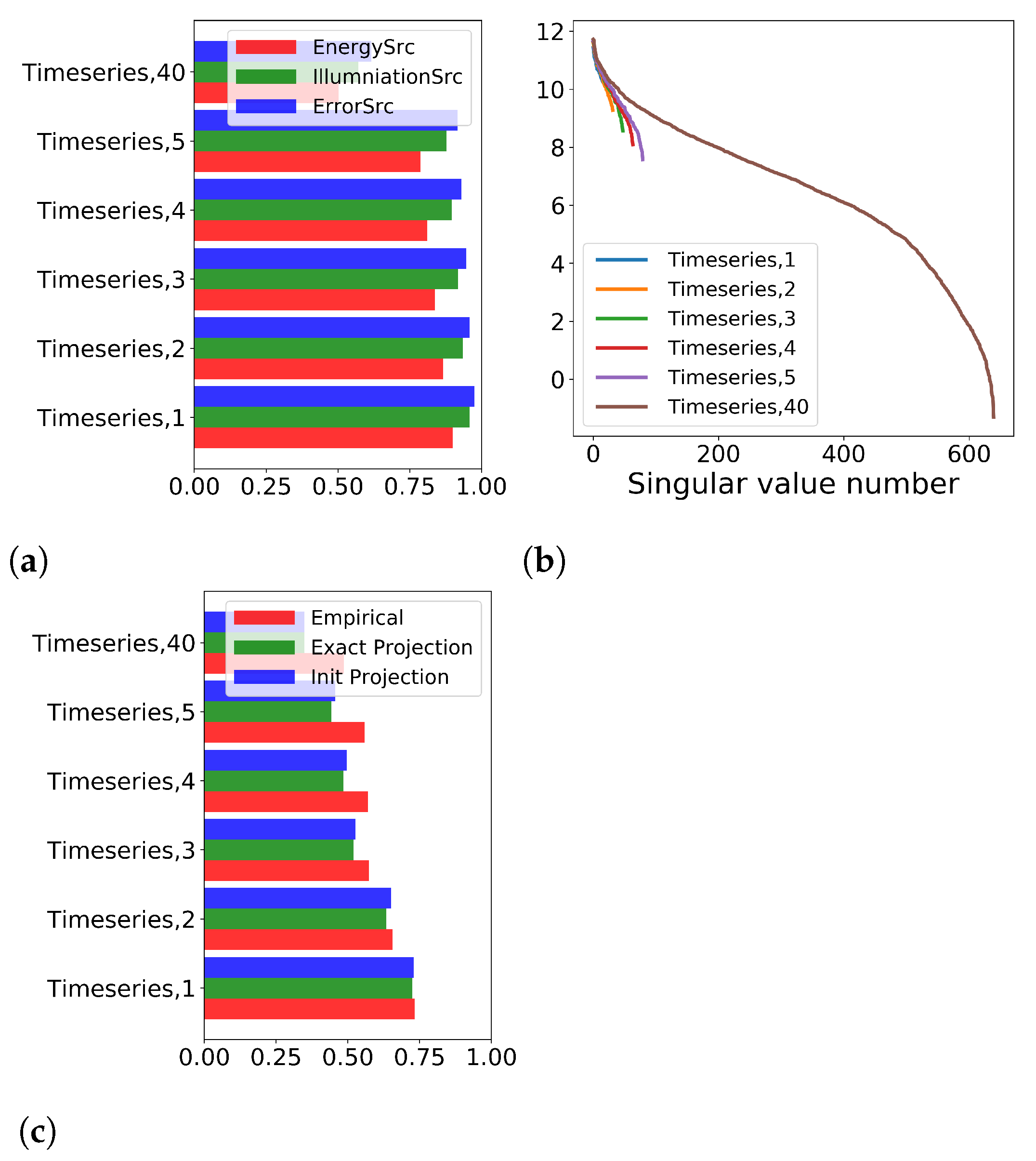
• “Timeseries”: $N_{Timeseries}$ time series of concentrations of the specific species in the specific points. In the state function terms:

  $$\left\{{\phi }_{l^{\left(m\right)}}(x^{\left(m\right)},t),t\in \left[0,T\right],\left(x^{\left(m\right)},l^{\left(m\right)}\right)\in {\left(\Omega \times L\right)}_{meas},m=1,\dots ,N_{Timeseries}\right\}.$$
  Projection system:

  $$h^{\left(\xi \right)}=C(T,{\theta }^{\left(\xi \right)},t)\delta (x-x^{\left(\xi \right)})\delta (l-l^{\left(\xi \right)}),\xi =1,\dots ,{\Xi }_{Timeseries}.$$
  For any element of $\left(x^{\left(m\right)},l^{\left(m\right)}\right)$, the parameter $\theta$ ranges from 0 to ${\Theta }_{Timeseries}-1$. The number of the frequencies ${\Theta }_{Timeseries}$ is the parameter of the projection system. This parameter is responsible for the temporal resolution of the considered data. Hence the total number of projection functions corresponding to the Timeseries is

  $${\Xi }_{Timeseries}={\Theta }_{Timeseries}\times N_{Timeseries}.$$
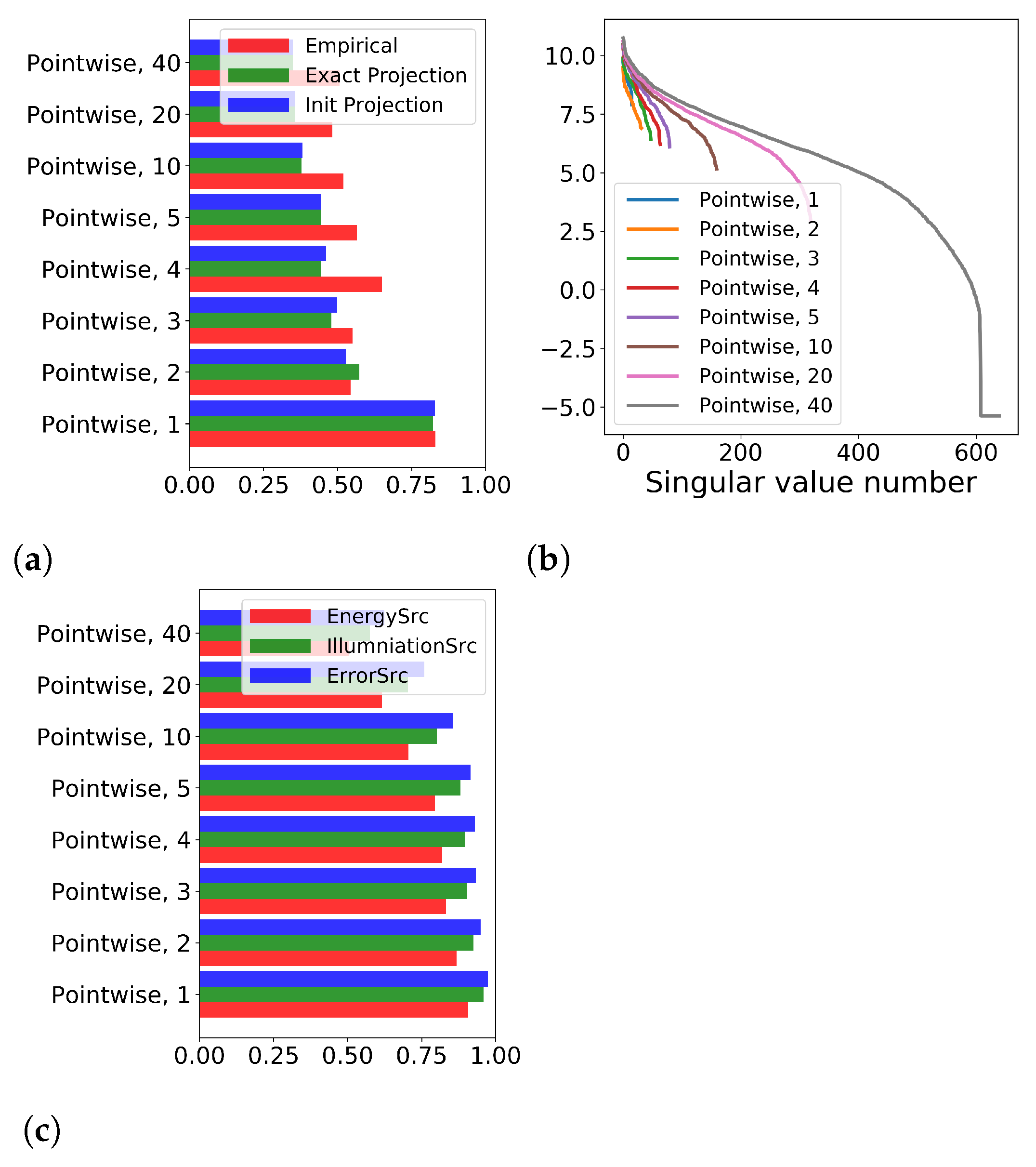
• “Pointwise”: $N_{Pointwise}$ Pointwise concentration measurements of the specific species at specific moments and specific points. In the state function terms:

  $$\left\{{\phi }_{l^{\left(m\right)}}(x^{\left(m\right)},t^{\left(m\right)}),\left(x^{\left(m\right)},t^{\left(m\right)},l^{\left(m\right)}\right)\in {\left({\Omega }_T\times L\right)}_{meas},m=1,\dots ,N_{Pointwise}\right\}.$$
  Projection system:

  $$h^{\left(\xi \right)}=\delta (x-x^{\left(\xi \right)})\delta (t-t^{\left(\xi \right)})\delta (l-l^{\left(\xi \right)}),\xi =1,\dots ,{\Xi }_{Pointwise}.$$
  The projection system is naturally defined by the measurement points. Hence the total number of the projection functions is ${\Xi }_{Pointwise}=N_{Pointwise}$. In the case of a large number of points, these data can be aggregated.
• “Integral”: $N_{Integral}$ Integrals of concentrations over the time interval of the specific species in the specific points. In the state function terms:

  $$\left\{{\int }_0^T{\phi }_{l^{\left(m\right)}}(x^{\left(m\right)},t)dt,\left(x^{\left(m\right)},l^{\left(m\right)}\right)\in {\left(\Omega \times L\right)}_{meas},m=1,\dots ,N_{Integral}\right\}.$$
  Projection system:

  $$h^{\left(\xi \right)}=\delta (x-x^{\left(\xi \right)})\delta (l-l^{\left(\xi \right)}),\xi =1,\dots ,{\Xi }_{Integral}.$$
  Here ${\Xi }_{Integral}=N_{Integral}$. Integral measurements are equivalent to “Timeseries” measurements with ${\theta }^{\left(\xi \right)}=0$.
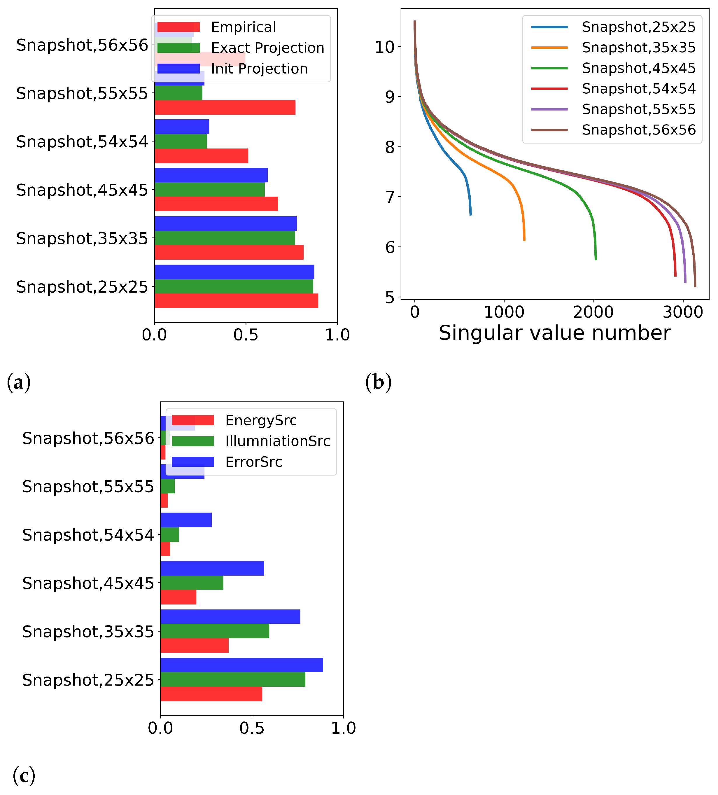
• “Snapshot”: $N_{Snapshot}$ specific species concentration fields images at specific moments in time. In the state function terms:

  $$\left\{{\phi }_{l^{\left(m\right)}}(x,t^{\left(m\right)}),x\in \Omega ,\left(t^{\left(m\right)},l^{\left(m\right)}\right)\in {\left(\left[0,T\right]\times L\right)}_{meas},m=1,\dots ,N_{Snapshot}\right\}.$$
  Projection system:

  $$h^{\left(\xi \right)}=C(X,{\theta }_x^{\left(\xi \right)},x)C(Y,{\theta }_y^{\left(\xi \right)},y)\delta (t-t^{\left(\xi \right)})\delta (l-l^{\left(\xi \right)}),\xi =1,\dots ,{\Xi }_{Snapshot}.$$
  The projection system has two parameters: ${\Theta }_{Snapshot}^{\left(x\right)}$ and ${\Theta }_{Snapshot}^{\left(y\right)}$, which define the spatial resolution of the considered data. For any image, ${\theta }_x$ and ${\theta }_y$ range in $0,\dots ,{\Theta }_{Snapshot}^{\left(x\right)}-1$ and $0,\dots ,{\Theta }_{Snapshot}^{\left(y\right)}-1$, respectively. Hence ${\Xi }_{Snapshot}=$$N_{Snapshot}\times {\Theta }_{Snapshot}^{\left(x\right)}\times {\Theta }_{Snapshot}^{\left(y\right)}$.

In the numerical algorithm, the operator Equation (8) is transformed to the discrete form. Hence, the projection functions are also substituted by their discrete analogs. To unify the scales of the different projection functions [57], their discrete analogs are normalized with respect to a discrete version of scalar products (6). This normalization makes any element of measurement data equally important. To make some elements more important than others, they can be additionally weighted.

2.4. Sensitivity-Operator-Based Analysis of Measurement System

Considering the quasi-linear representation (8) of the inverse problem data, we compare the following sensitivity-operator-based measurement system analyses.

2.4.1. Inverse Problem Solution

The basic way to evaluate the informative content of the measurement data is to directly compare the result of solving (8) by a source identification algorithm with the known exact solution. The better the reconstruction, the more information is contained in the data. However, this estimation method requires a complete setting of the inverse modeling scenario (including the “exact” emission source), an appropriate algorithm of source identification, and enough time and computational capacities to solve the inverse problem. We call this approach “empirical”.

The procedure of evaluating the measurement system is carried out according to the following scheme:

(1)

The “exact” solution ${\mathbf{q}}^{(*)}$ is given. In our case, this is the location and capacity of the emission sources.

(2)

The “exact” solution ${\mathbf{q}}^{(*)}$ is then used to simulate the “measurement data“. This “measurement data” is used in the algorithm to solve the inverse problem.

(3)

The result ${\mathbf{q}}^{(\infty )}$ of the algorithm is compared with the “exact” solution. In this case, both the reconstruction of the source is estimated, and the convergence parameters of the algorithm are analyzed.

This estimation strongly depends on the source identification algorithm, which may have its features. For example, it can be locally convergent, and therefore, dependent on the initial guess.

2.4.2. Sensitivity Operator Properties Analysis

The quasi-linear inverse problem representation (8) can be used to predict the quality of solving the inverse problem prior to solving it [39,41]. Indeed, if we assume that $M_U[{\mathbf{q}}^{(*)},\mathbf{q}]$ is known or is weakly dependent on ${\mathbf{q}}^{(*)}$, then Equation (8) becomes a linear ill-posed operator equation, and we can use linear theory to evaluate the inverse problem properties.

Let there be grid domains ${\Omega }^h$ and ${\Omega }_T^h$, corresponding to $\Omega$ and ${\Omega }_T$, and a map that encodes a grid point with coordinates $(x_i,y_j,l)\in {\Omega }^h\times L_{src}$ by a single index. Let $N_x,N_y$ be the numbers of grid points of ${\Omega }^h$ in the x and y dimensions, respectively. In the rest of the paper, we work with the discretized versions of the considered aggregates. Hence we can consider $\mathbf{q}$ as the vector from ${\mathbb{R}}^{N_x{N}_y\left|L_{src}\right|}$. Here, $|L_{src}|$ means the number of elements in $L_{src}$. The sensitivity operator $M_U[{\mathbf{q}}^{(*)},\mathbf{q}]$ can be considered as the matrix ${\mathbb{R}}^{\Xi \times \left(N_x{N}_y\right|L_{src}\left|\right)}$.

In the theory of ill-posed problems, the linearized version of the operator Equation (8) in the neighborhood of the exact solution:

$$M({\mathbf{q}}^{(*)}-\mathbf{q})\approx f_M,f_M:=H_{U}I-H_U\mathbf{\phi }\left[\mathbf{q}\right],M:=M_U[{\mathbf{q}}^{(*)},{\mathbf{q}}^{(*)}]$$

is considered. According to p. 49 in [72], regularization algorithms search for the best approximate solution of $\delta {\mathbf{q}}^{†}$, which in our case is defined as:

$$\delta {\mathbf{q}}^{†}={\left(M^{*}M\right)}^{†}{M}^{*}{f}_M\approx {\left(M^{*}M\right)}^{†}\left(M^{*}M\right)({\mathbf{q}}^{(*)}-\mathbf{q}),$$

(9)

where ${\left(M^{*}M\right)}^{†}$ is the generalized Moore–Penrose inverse for $M^{*}M$. The aggregate $M^{*}M$ is the Fisher information matrix. The aggregate ${\left(M^{*}M\right)}^{†}\left(M^{*}M\right)$ is an orthogonal projector on the orthogonal complement to the sensitivity operator’s kernel. Indeed, if the singular value decomposition of M is $\{U,S,V\}$ and for any z:

$$Mz=\sum _{n=1}^N{U}_n{s}_n〈V_n,z〉,$$

where N is the number of nonzero singular vectors. Then,

$$M^{*}Mz=\sum _{n=1}^N{V}_n{s}_n^2〈V_n,z〉,{\left(M^{*}M\right)}^{†}z=\sum _{n=1}^N{V}_n\frac{〈V_n,z〉}{s_n^2},$$

and

$${\left(M^{*}M\right)}^{†}\left(M^{*}M\right)z=\sum _{n=1}^N{V}_n〈V_n,z〉.$$

Roughly speaking, only the projection of ${\mathbf{q}}^{(*)}-\mathbf{q}$ on the nonzero right singular vectors of the sensitivity operator matrix can be restored at best because the rest of the information about the uncertainty variation is lost.

The disadvantage of using ${\left(M^{*}M\right)}^{†}\left(M^{*}M\right)$ in the source identification problem is that the dimensionality of $M^{*}M$, which has to be pseudo-inverted, is the (number of unknowns × number of unknowns), which is as large as $N_x{N}_y\left|L_{src}\right|$. Another way to express the projector is to use the equivalent (Appendix B) aggregate:

$$M^{*}{\left(M{M}^{*}\right)}^{†}Mz=\sum _{n=1}^N{V}_n〈V_n,z〉.$$

(10)

In this case, the matrix $M{M}^{*}$ has the dimensionality (number of adjoint ensemble members × number of adjoint ensemble members) or $\Xi \times \Xi$, which is under our control. The representation (10) is more useful when the number of adjoint ensemble members is less than the number of unknowns, and therefore, we use it in our calculations. Let:

$$\mathsf{{\rm Y}}[{\mathbf{q}}^{\left(2\right)},{\mathbf{q}}^{\left(1\right)}]:=M^{*}{\left(M{M}^{*}\right)}^{†}M,$$

where $M=M[{\mathbf{q}}^{\left(2\right)},{\mathbf{q}}^{\left(1\right)}]$. As the first predictor of the solution, we consider:

$${\mathbf{q}}^{\left(p\right)}:={\mathbf{q}}^{\left(0\right)}+\mathsf{{\rm Y}}[{\mathbf{q}}^{\left(0\right)},{\mathbf{q}}^{\left(0\right)}]\left({\mathbf{q}}^{\left(*\right)}-{\mathbf{q}}^{\left(0\right)}\right).$$

(11)

Another estimate that seems to be even more appropriate is:

$${\mathbf{q}}^{\left(e\right)}:={\mathbf{q}}^{\left(0\right)}+\mathsf{{\rm Y}}[{\mathbf{q}}^{\left(*\right)},{\mathbf{q}}^{\left(0\right)}]\left({\mathbf{q}}^{\left(*\right)}-{\mathbf{q}}^{\left(0\right)}\right).$$

(12)

Estimates (11) and (12) take the exact solution ${\mathbf{q}}^{\left(*\right)}$, and it takes less time to evaluate them than solving the inverse problem with an algorithm.

Let us consider the properties of $\mathsf{{\rm Y}}=\mathsf{{\rm Y}}[{\mathbf{q}}^{\left(0\right)},{\mathbf{q}}^{\left(0\right)}]$, which are independent of the exact solution. In the ideal case, $\mathsf{{\rm Y}}$ should be equal to the identity operator $Id$. It means that the sources can be potentially reconstructed exactly. If we apply this operator to a single source with a unitary emission rate located in the $\kappa$-th point, we obtain the result of its representation by the monitoring system. This single source corresponds to the vector ${\left[Id\right]}_{\kappa }$ with only one unitary element on the $\kappa$-th place. In the inverse modeling scenario (see Section 2.5), we deal with the Pointwise sources and ${\left[\mathsf{{\rm Y}}\right]}_{\kappa }=\mathsf{{\rm Y}}{\left[Id\right]}_{\kappa }$. Hence, the $\kappa$-th column of $\mathsf{{\rm Y}}$ describes how the unitary source, located in the $\kappa$-th point of the grid domain, is transformed by the inverse problem. In the ideal case, ${\left[\mathsf{{\rm Y}}\right]}_{\kappa }$ should be equal to ${\left[Id\right]}_{\kappa }$.

We can characterize the difference between ${\left[\mathsf{{\rm Y}}\right]}_{\kappa }$ and ${\left[Id\right]}_{\kappa }$ on the Pointwise basis with several meaningful characteristics linked to the structure and interpretation of $\mathsf{{\rm Y}}$. The first characteristic is:

$$E_{\kappa }^{\left(n\right)}=\parallel {\left[Id\right]}_{\kappa }-{\left[\mathsf{{\rm Y}}\right]}_{\kappa }\parallel .$$

(13)

If the information about the source in the $\kappa$-th point is lost completely, then the norm $∥{\left[\mathsf{{\rm Y}}\right]}_{\kappa }∥$ is zero. In the ideal case, $∥{\left[\mathsf{{\rm Y}}\right]}_{\kappa }∥=1$. We consider the following error-type characteristic:

$$E_{\kappa }^{\left(e\right)}=1-∥{\left[\mathsf{{\rm Y}}\right]}_{\kappa }∥,$$

(14)

To evaluate the characteristics $E_{\kappa }^{\left(n\right)}$ and $E_{\kappa }^{\left(e\right)}$, we have to evaluate the complete $\mathsf{{\rm Y}}$ matrix. Let us look at the characteristics that are evaluated with the reduced amount of $\mathsf{{\rm Y}}$’s elements. In [19], there is an aggregate called “Illumination” and it is expressed as:

$${\left[M\right]}_{\kappa }^{*}{\left(M{M}^{*}\right)}^{†}{\left[M\right]}_{\kappa }={\left[\mathsf{{\rm Y}}\right]}_{\kappa \kappa },$$

(15)

where ${\left[\mathsf{{\rm Y}}\right]}_{\kappa \kappa }$ is the $\kappa$-th diagonal element of $\mathsf{{\rm Y}}$. Since $\mathsf{{\rm Y}}$ is equal to $Id$ in the ideal case, hence ${\left[\mathsf{{\rm Y}}\right]}_{\kappa \kappa }$ should be equal to 1. We consider the error-type characteristic:

$$E_{\kappa }^{\left(i\right)}=1-{\left[M\right]}_{\kappa }^{*}{\left(M{M}^{*}\right)}^{†}{\left[M\right]}_{\kappa }.$$

(16)

Let us consider the application of $\mathsf{{\rm Y}}$ to the set of sources of interest $\left\{{\left[Id\right]}_{\kappa },\kappa \in K\right\}$. For example, K can be a priori known source locations or the whole domain. We can evaluate characteristics (13), (14), and (16) on K. Corresponding cumulative characteristics are:

$$E^{\left(c\right)}=\frac{1}{\left|K\right|}\sum _{\kappa \in K}{E}_{\kappa }^{\left(c\right)},c\in \{n,e,i\}.$$

(17)

The analysis tool that does not take knowing the exact solution is the decay rate of the sensitivity operator singular spectrum ${\left\{s_n\right\}}_{n=1}^N$, as it is done in [73]. The issue with this analysis type is how to compare different singular spectra quantitatively.

2.5. Inverse Modeling Scenario

Constructing a realistic inverse modeling scenario is an essential part of inverse modeling. In the context of the source identification problem, the main components of an inverse modeling scenario are:

• Geographical domain.
• Monitoring system characteristics: locations and accuracy.
• Main emission sources to construct the “exact” solution.
• Chemical transformation mechanism, initial, and boundary conditions.
• Meteorological conditions, determining CTM model coefficients.

The geographical domain (Figure 1) is the most definite component of the scenario. The monitoring system is also a definite component of the inverse modeling scenario since the positions of all the monitoring sites are known. The locations of some Roshydromet sites [48] (Figure 1) were taken as the prototype of the measurement system in the scenario. According to [48], the system measures several components, including $S{O}_2$, $CO$, $N{O}_2$, $NO$, $O_3$, $HS$, $P{M}_{2.5}$, and $P{M}_{10}$. The measurement data is provided in the open-access mode on a daily-averaged basis. In the scenario, we suppose that there are only $O_3$ concentration measurements ($L_{meas}=\{\#\left(O_3\right)\}$). Here $\#\left(O_3\right)$ denotes the index of $O_3$ concentration in the state function $\mathbf{\phi }$. The types of measurements collected at the measurement sites are defined in the numerical experiments.

In the considered scenario, the images (Snapshots) cover the whole domain simultaneously. The geostationary satellites can potentially obtain this type of image [74,75]. Nevertheless, the instant image of the whole domain is a simplification since each instrument has its spatial and temporal resolution and coverage. Non-geostationary satellites collect images as the series of smaller images along their tracks with a given swath width [76,77,78]. More details about the satellite images of the concentration fields can be found in [74,75,76,77,78]. In our scenario, the images of the concentration field are available on the third day of the period ($t=3\times 24\times 3600$ s).

Emission sources are the factor that largely determines the air quality in the region, but the information about the sources is incomplete. This is the main reason for developing the source identification algorithms. We need to construct a realistic “exact” solution to move in this direction. It will be required to check the source identification algorithms (see Section 2.4.1) and to provide the estimate of ${\mathbf{q}}^{(*)}$ to evaluate the sensitivity operator $M_U\left[{\mathbf{q}}^{(*)},\mathbf{q}\right]$ for the analysis purposes (see Section 2.4.2).

We construct the “exact” solution as a set of Pointwise sources with constant time emission rates. Furthermore, we suppose that the only emitted substance is $NO$ ($L_{src}=\{\#\left(NO\right)\}$). In this scenario, we have so-called “indirect” measurements, when the measured substance ($O_3$) is different from the emitted one ($NO$).

To define realistic emission rates, we depart from the estimate ${\overline{q}}_{NO}^{\left(Irkutsk\right)}$ of the Irkutsk (the largest city in the region) total production of $NO$ from [65]:

$${\overline{q}}_{NO}^{\left(Irkutsk\right)}=125\times {10}^3\frac{mg}{s}.$$

(18)

To obtain the concentration change in the grid cell due to the emissions, we divide ${\overline{q}}_{NO}^{\left(Irkutsk\right)}$ by the volume of the grid cell $V_{cell}$ in m${}^3$:

$$\begin{array}{c}{V}_{cell}=19502\times 21991.6\times 100m^3,\\ q_{NO}^{\left(Irkutsk\right)}\approx 2.91\times {10}^{-6}\frac{mg}{s{m}^3}.\end{array}$$

In the figures, we use the dimensionality $\frac{mg}{s{m}^3}$ for the sources and $\frac{mg}{m^3}$ for the concentrations.

The emission of the c-th city in the region is estimated as proportional to the ratio of its population to Irkutsk’s population:

$$q_{NO}^{\left(c\right)}=q_{NO}^{\left(Irkutsk\right)}\times \frac{Populatio{n}^{\left(c\right)}}{Populatio{n}^{\left(Irkutsk\right)}},$$

(19)

where $Populatio{n}^{\left(c\right)}$ is the population in the c-th city according to Wolfram Alpha Service [79]. This construction of the scenario allows obtaining a spatially heterogeneous distribution of the unequal emission sources.

The city’s emissions are attributed to the nearest grid-point. If more than one city corresponds to a grid point, then the emissions of these cities are added. We call this configuration a “realistic” source configuration (Figure 2a). In the second configuration (Figure 2c) all the cities have identical emission rates, while the total of the emission rates is the same as in the “realistic” source configuration. We call it a “unified” configuration. In the third configuration (Figure 2e) all the emissions from the “realistic” configuration are localized in the nearest grid-point to the Irkutsk city. We denote this configuration by a “single”. All these source configurations have the same $L_1$ norm. The initial guess for the source identification is zero emissions. Therefore, the relative error of the initial guess is $100\%$. A priory emission source is considered as zero $\mathbf{f}=0$.

Along with the anthropogenic sources, the sources and sinks are determined by the natural processes: rains and snowfalls, vegetation, forest fires, swamps, etc. The chemical reactions, unconsidered in the transformation model, also contribute to the distributed sources and sinks. These sources are not addressed in the paper since we use only synthetic data. In the case of the real measurement data, these sources should also be taken into consideration. The primary anthropogenic emission sources and the natural factors define the chemical transformation model to be considered. Since the inverse modeling tasks are time-consuming, the chemical system should be as small as possible but relevant to the main chemical components, especially the major primary and secondary pollutants.

As the transformation model (operators P and $\Pi$ in (1)), we chose the Leighton relationship-based atmospheric chemistry model (e.g., [80]), described in Appendix C. Initial conditions ${\phi }_l^0$ are taken as constant in space according to (A11)–(A13). This simplification can be refined by using the output of the global chemical transport models (e.g., [81]) or setting the model’s spin-up period. The boundary conditions are:

$${\alpha }_l=\left\{\genfrac{}{}{0.0pt}{}{0,(\mathbf{x},t)\in {\Gamma }^{\left(out\right)}}{{\phi }_l^0,(\mathbf{x},t)\in {\Gamma }^{\left(in\right)}}\right.,{\beta }_l=0,$$

(20)

where ${\phi }_l^0$ is the constant value of the corresponding initial conditions. The values of ${\phi }_l^0$ denote background concentrations of the considered substances. This simplification can also be refined by taking the output of the global CTMs as the boundary conditions.

Meteorological conditions are the most variable component in the system. Modern meteorological models can evaluate the meteorological fields with high accuracy. The weather data for the scenario was chosen for the period from 12:00 on 23.07.2019 to 12:00 on 26.07.2019. The results of the COSMO (Consortium for Small-scale Modeling) model calculation [82] are used as the 2D wind-speed vector field $\mathbf{u}$ at the surface level. The description of the meteorological conditions is given in Appendix D. The diffusion coefficient $\mu =1000$ m${}^2$/s was chosen as a constant one.

To generate the “exact” solution ${\phi }^{(*)}$, we solve the direct problem. The $O_3$ elements of the “exact” solution are used to obtain the synthetic measurement data. To show the differences between the source configurations, we present mean (over time interval $[0,T]$) $NO$ concentration fields in Figure 2b,d,f.

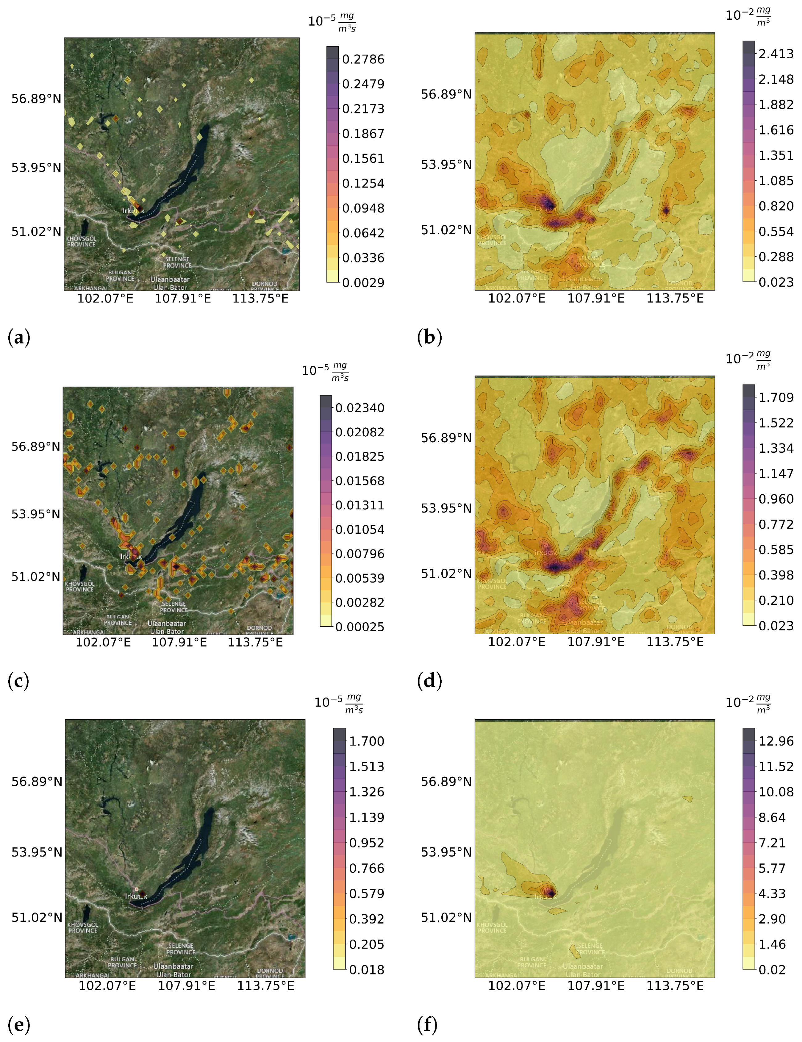
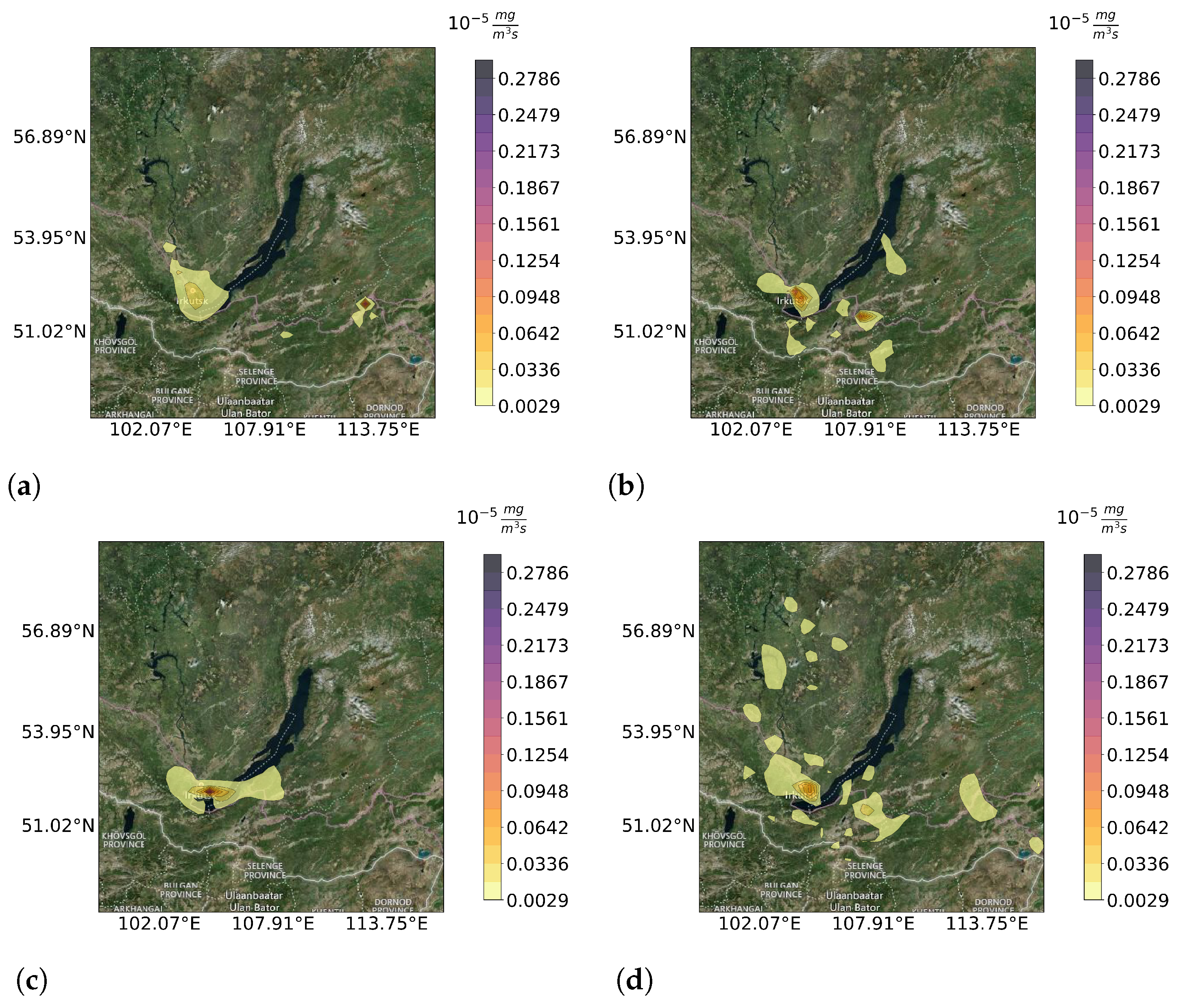
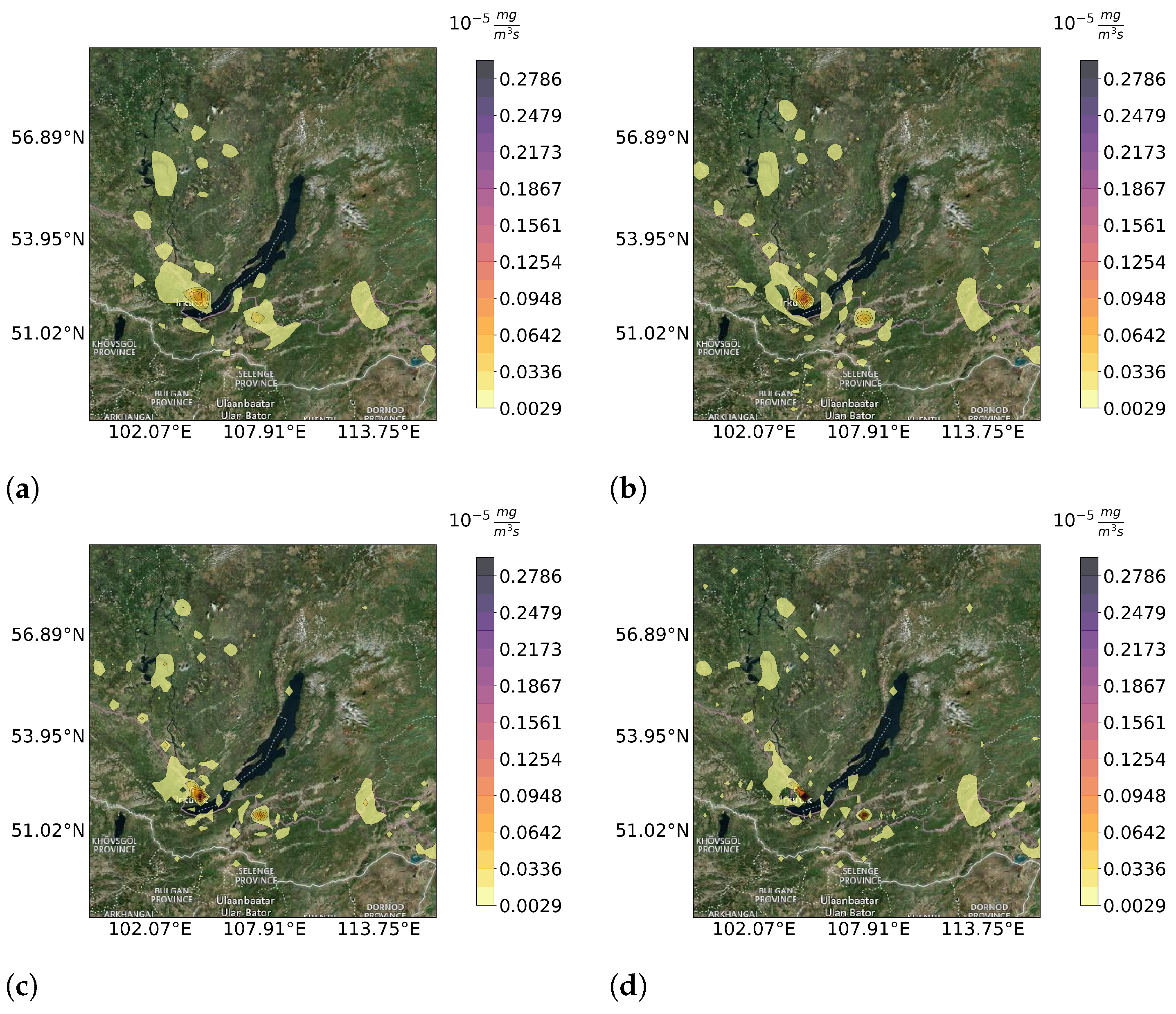
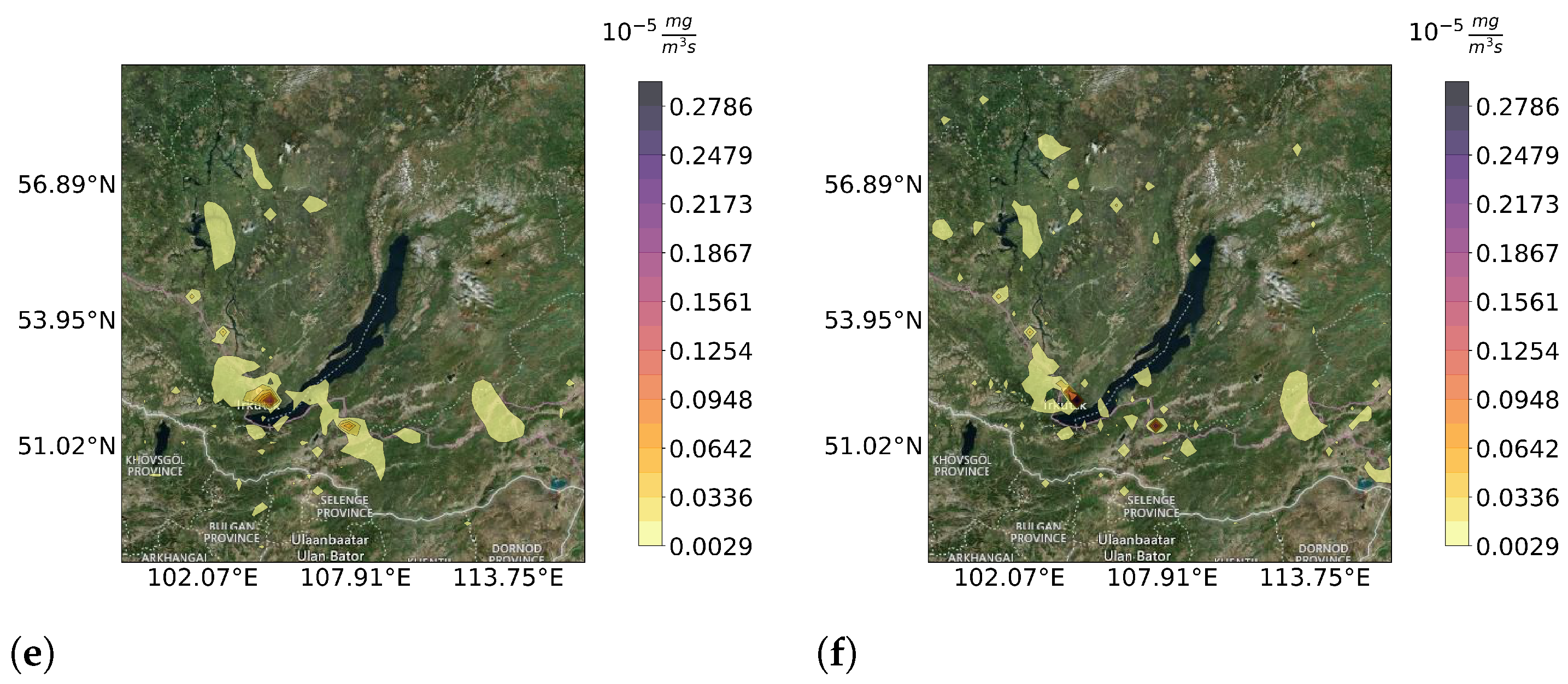
3. Results

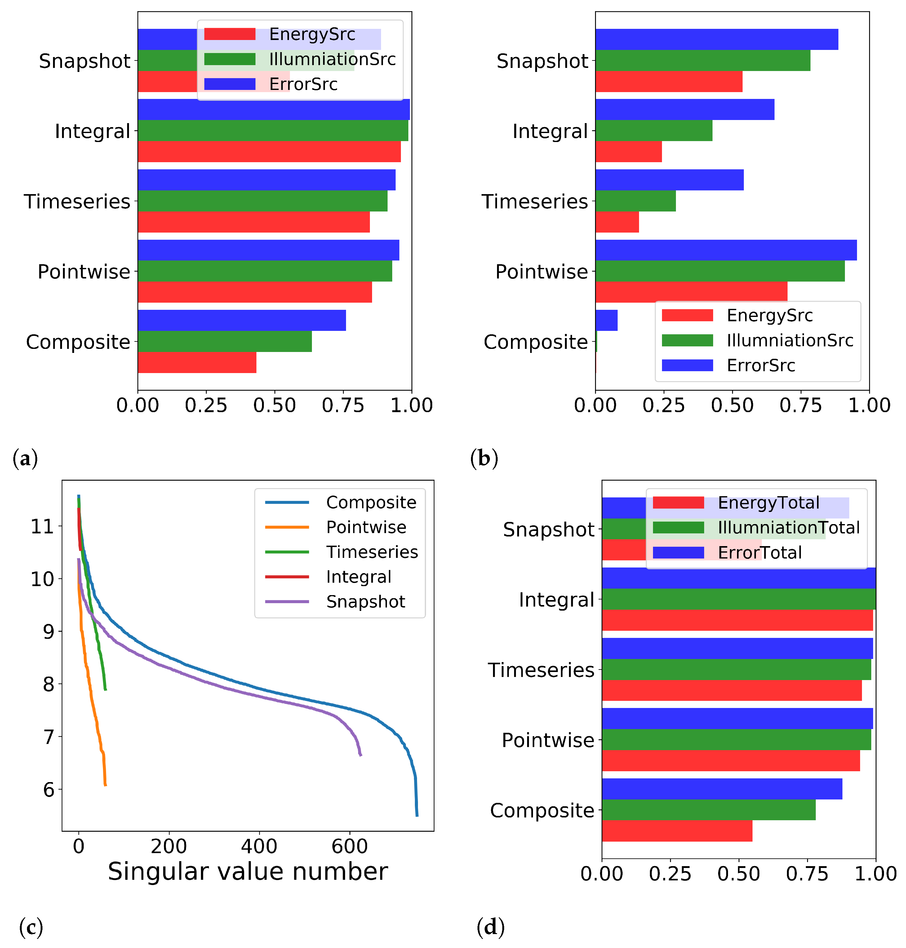
3.1. Heterogeneous Measurements

To evaluate the synergistic effect of using different measurement types, we compare the source identification (or simply reconstruction) results obtained for composite measurements with those obtained for the specialized measurement types. The measurement sites are divided into three groups (Figure 1): Timeseries, Pointwise, and Integral. In the considered configurations, we use the parameters of the projection functions ensembles given in

Table 1. Adjoint ensemble sizes.

Type	${\Xi }_{\mathbf{Type}}$	${\mathit{N}}_{\mathbf{Type}}$	Description
Pointwise	60	60	$5\mathrm{sites}\times 12\mathrm{measurement}\mathrm{moments}$
Timeseries	60	6	$6\mathrm{sites}\times 10,{\Theta }_{Timeseries}=10$
Integral	5	5	$5\mathrm{sites}$
Snapshot	625	1	$1\mathrm{image}\times 25\times 25,{\Theta }_{Snapshot}^{\left(x\right)}={\Theta }_{Snapshot}^{\left(y\right)}=25$
Composite	750		Sum of the above

. Pointwise measurements are taken at 6-hour time intervals.

The source reconstruction results for individual measurement types in the “realistic” source configuration are presented in Figure 3. We see that the positions of “Pointwise” measurements are far from the largest source cluster located near Irkutsk. Respectively, the reconstruction by “Pointwise” measurements is less accurate for this cluster compared to other measurement types. Snapshot reconstruction allows one to identify the sources that are far from the air quality monitoring network. Still, it contains many artifacts explainable by a relatively small number of the projection functions.

In Figure 4, we compare composite data reconstruction results for different source configurations. In Figure 5, the relative errors in different measurement configurations and their estimates are presented. Here “empirical” denotes the error obtained with the inverse problem solution algorithm; “init projection”, and “exact projection” denote the errors of the estimates (11) and (12), respectively. The less is the red (“empirical”) bar, the better the solution is. Since “init projection” (blue bars) and “exact projection” (green bars) are the estimates of the “empirical” relative error, then in the ideal case, they should have the same lengths as the red bar. As we can see, projections (11) and (12) give a relatively accurate estimate of the inverse problem solution.

Comparing the different source configuration results, we can see that the best reconstructions for the composite measurements are obtained for “realistic” and “single” emission sources. The best “Snapshot” results are obtained for the “unified” sources configuration. The localized measurements (Pointwise, Timeseries, Integral) are taken near the most populated cities in the region. In the “realistic” and “single” source configurations, they provide better reconstruction than in the “unified” case. In the “unified” case, the location of the measurements plays a less important role, and the “Pointwise” reconstruction results are comparable to the “Timeseries” results.

In Figure 6, we compare the characteristics that do not know the exact emission rates. Here “EnergySrc”, “ErrorSrc”, and “IlluminationSrc” denote $E^{\left(e\right)}$, $E^{\left(n\right)}$, and $E^{\left(i\right)}$ from (17), respectively, for K containing the indices of the grid points with “cities”. “EnergyTotal”, “ErrorTotal”, and “IlluminationTotal” denote the same characteristics but for K containing all grid points indices. These characteristics are also considered as the estimates of the “empirical” relative error. The characteristics in Figure 6a,b take the information of the source positions. The characteristics in Figure 6c,d are completely independent of the information about the sources.

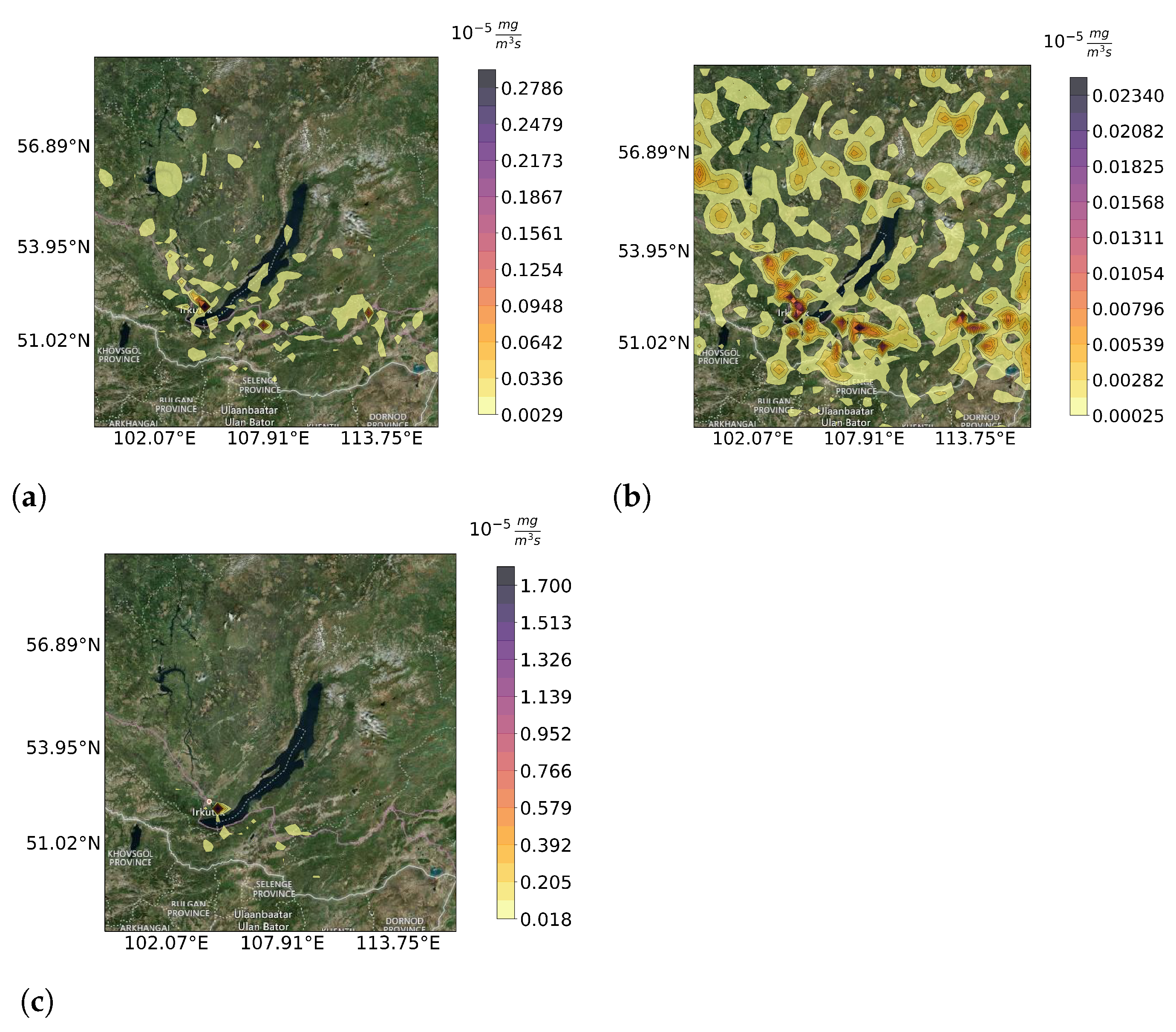
3.2. Specific Measurement Types

In these experiments, we compare the reconstruction results for the “realistic” source configuration in cases when the whole measurement network collects data of the same type. The second question is how the ensemble parameters (such as ${\Theta }_{Timeseries}$, ${\Theta }_{Snapshot}^{\left(x\right)}$, ${\Theta }_{Snapshot}^{\left(y\right)}$) influence the reconstruction results. In Figure 7, we present the results for different numbers of projection functions in the case of time-series measurements. The label on a figure “Timeseries, N” means that ${\Theta }_{Timeseries}=N$. In Figure 8, we compare the results of Pointwise measurements for different numbers of measurement acquisition times. The label on a figure “Pointwise, N” means that time series in each of 16 sites are approximated by N values uniformly distributed on the time interval, i.e., for “Pointwise, 40” $\Xi =16\times 40$. In the last experiment (Figure 9), we consider reconstruction results for the different number of projection functions in the Snapshot case. The label on a figure “Snapshot, $N\times N$” means that ${\Theta }_{Snapshot}^{\left(x\right)}=N$, ${\Theta }_{Snapshot}^{\left(y\right)}=N$. In Figure 10, we compare the reconstruction results for different numbers of the projection functions in the Snapshot scenario.

In Figure 11, we compare the reconstruction results for different measurement types. Timeseries configuration is presented for $\Xi =40\times 16$, Pointwise for $\Xi =40\times 16$, and Snapshot for $\Xi =56\times 56$. In Figure 12, we can see the projection-based estimates of the results in Figure 11. In Figure 13, there are the corresponding illumination functions (15).

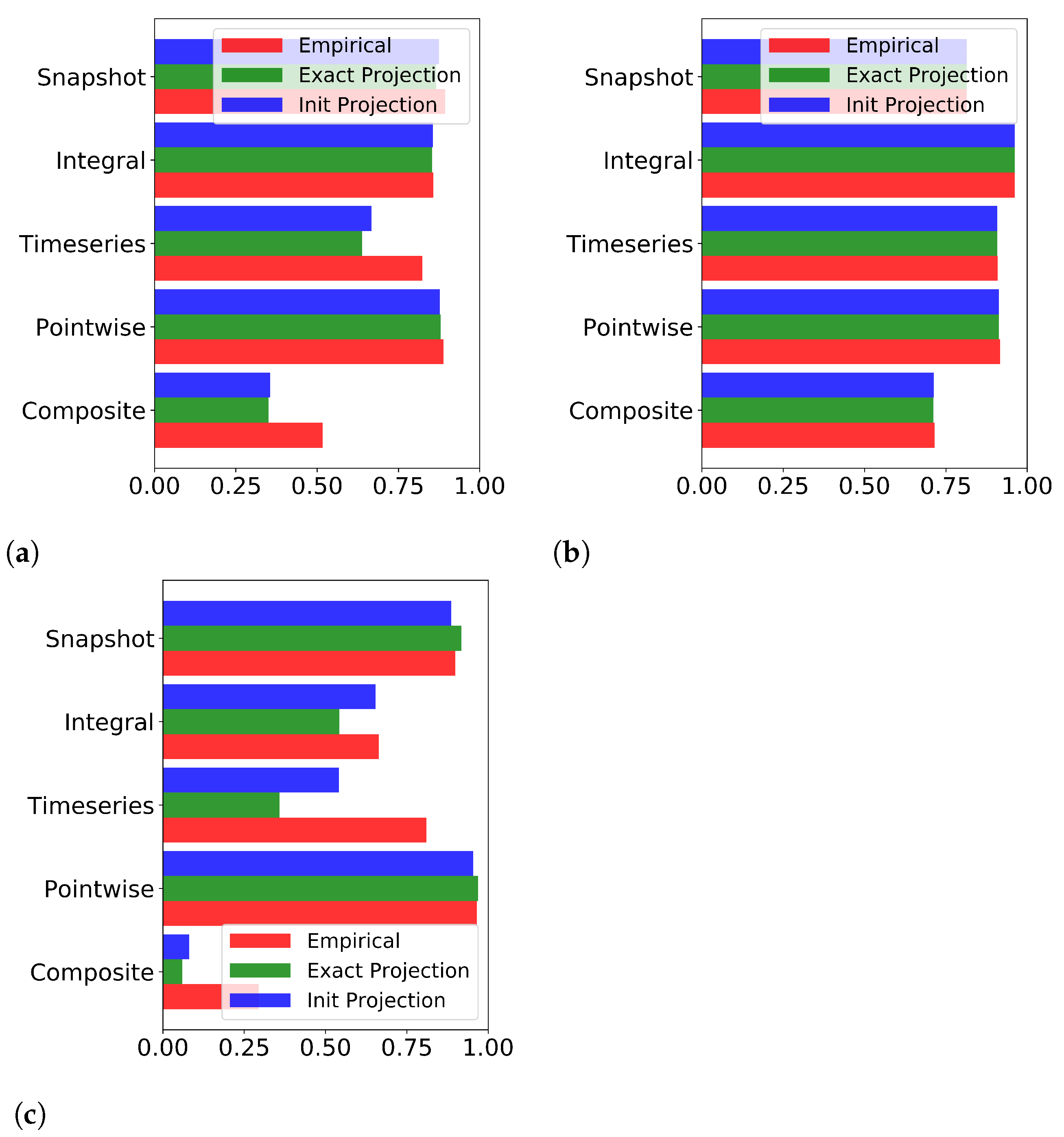
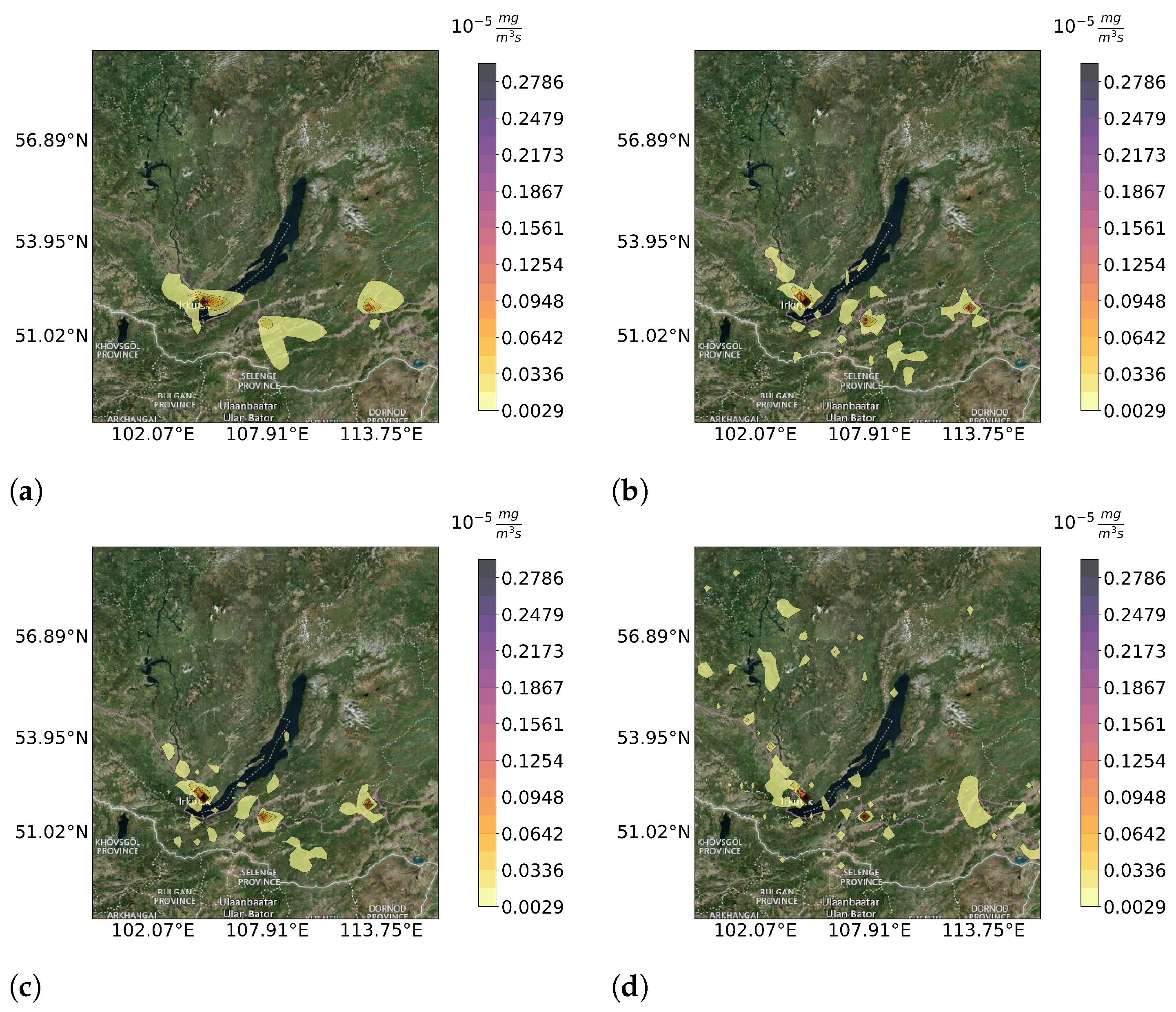
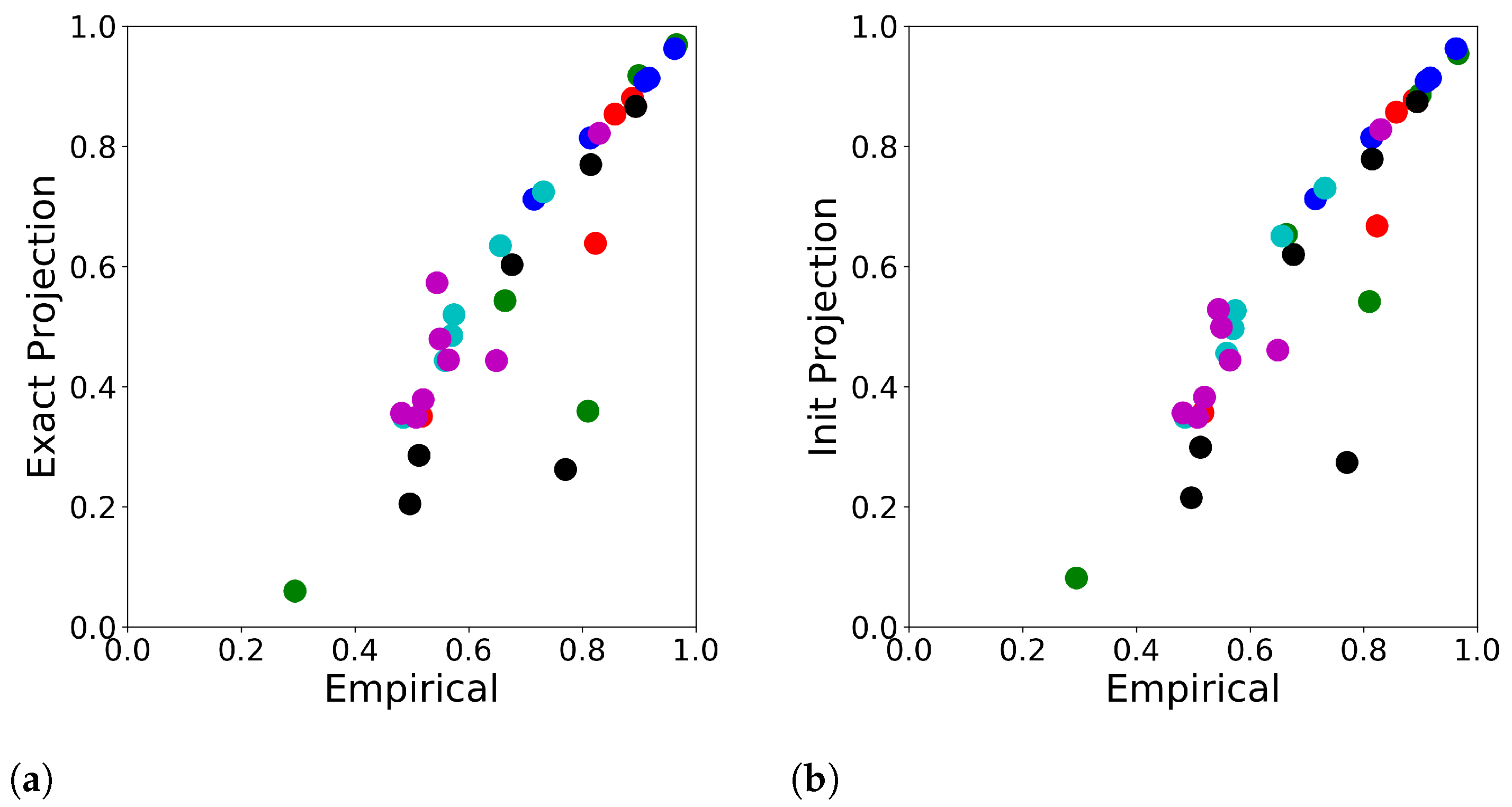
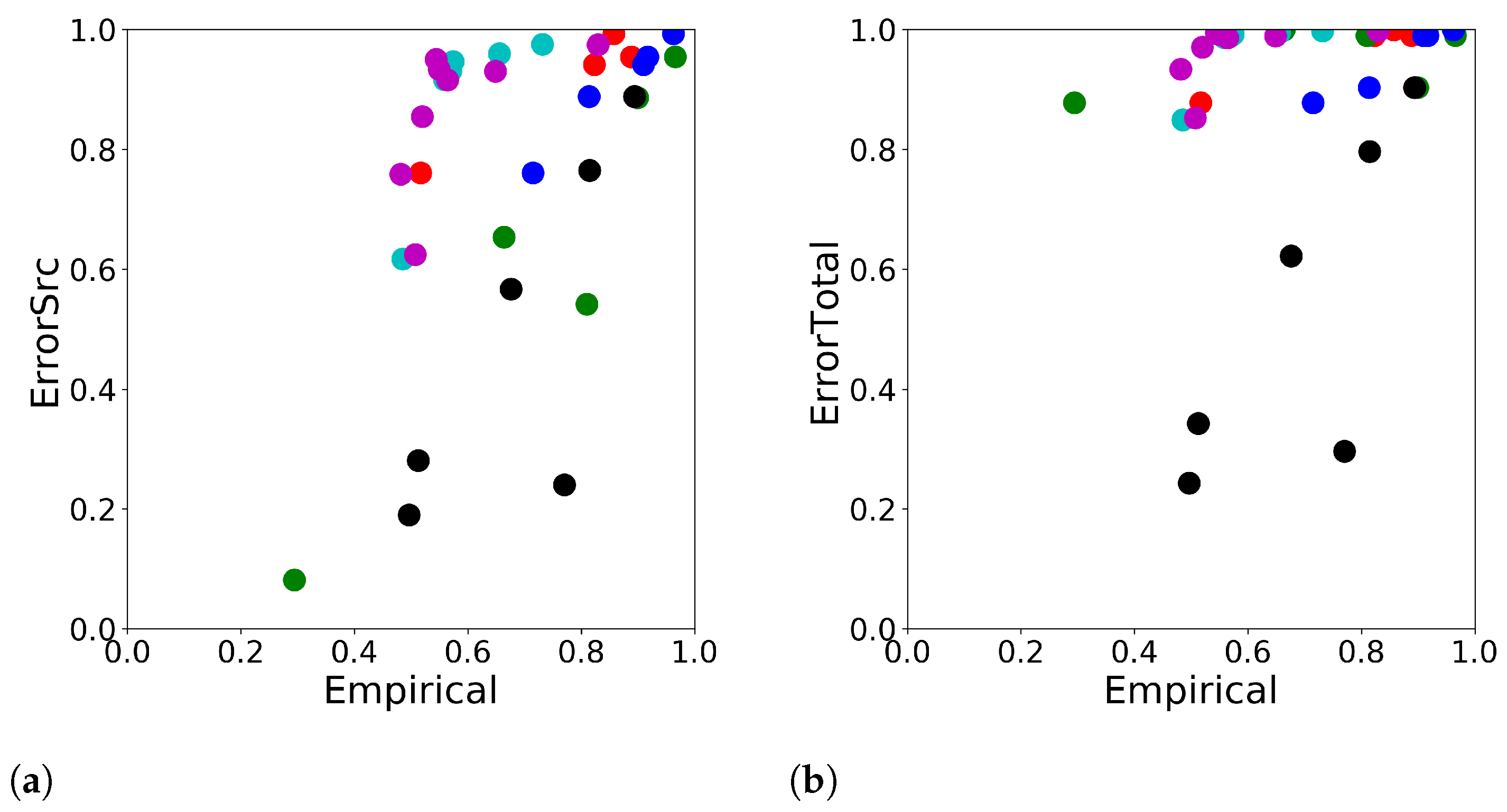
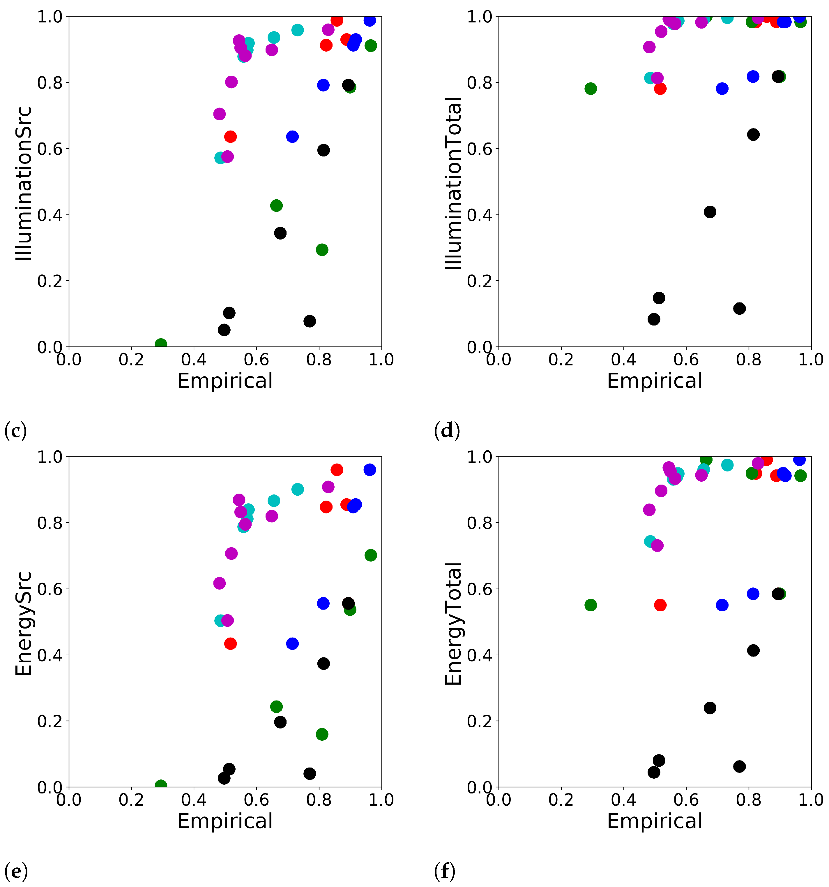
3.3. Accuracy of the Reconstruction’s Prediction

To summarize the relationship between the considered characteristics and the resulting “Empirical” source identification errors, we made the scatter plots in Figure 14 and Figure 15. The colors in Figures denote different experiments:

• Red: Section 3.1, “realistic” source case;
• Green: Section 3.1, “single” source case;
• Blue: Section 3.1, “unified” source case;
• Black: Section 3.2, Timeseries experiment;
• Cyan: Section 3.2, Pointwise experiment;
• Magenta: Section 3.2, Snapshot experiment.

In Figure 14, we present the characteristics that take the “Exact” solution. The characteristics in Figure 15a,c,e take the locations of the “Exact” sources. The characteristics in Figure 15b,d,f are entirely independent of the “Exact” solution.

4. Discussion

An essential advantage of the sensitivity-operator-based approach to inverse modeling is that various problems can be reduced in a unified way to a family of quasi-linear operator equations. Due to the properties of adjoint equations and sensitivity relations, the developed approach makes it possible to work in a unified way with heterogeneous measurement data. Note that these properties of the sensitivity relations are also used in the variational algorithms where various measurements can be combined by adding corresponding discrepancy functions to the cost function. However, in contrast, the sensitivity-operator-based approach also provides a straightforward way to analyze the inverse problem properties by analyzing the properties of the corresponding sensitivity operator family. Moreover, a sensitivity operator can combine not only different measurement types and their ensembles. If the source (or source pattern) persists for a long time, it may combine different meteorological scenarios to a single sensitivity operator.

Sensitivity functions are calculated with the adjoint equation’s solutions. The adjoint equation structure is determined by the equations in variations for the direct problem, i.e., by the process model. We do not discuss the limitations of the approach that are inherited from the process model here (1)–(4), since the air quality model development is a separate work direction, which deserves special attention. Nevertheless, the need to derive the adjoint problems for complicated models can also be considered as the limitation of the approach. This limitation can be alleviated by using automatic adjoint code generators [83,84,85].

In turn, the measurement data determine the sources for the adjoint equations. Hence, a limitation of the approach is that a measurement data element has to be presented as the application of the scalar-product-type aggregate to the model state function. This is a weak limitation in the case of the linear measurement operators, connecting the model’s state function with the measurement data. To consider nonlinear measurement operators, the adjoint problem has to be altered. This is a matter of further research.

Based on the sensitivity operator analysis of the inverse problem, methods of express analysis and refined analysis of the information content of monitoring systems data can be considered. The quasi-linear structure of the resulting operator equation admits using linear (matrix) analysis tools to estimate the inverse problem properties. Since solving the inverse problem may take a significant amount of time compared to the solution of the direct problem, it is advantageous to have an express estimate of the inverse problem solution quality that can be achieved in the given conditions. This is especially important for the monitoring system design (or optimization) task when one has to try and compare different system configurations. Our approach gives such a possibility straightforwardly.

On the other hand, the gain in computational time takes its payback. The difference between the “empirical” relative error and its estimates can be considered as the limitation of the approach. To overcome this limitation, we recommend checking the conclusions obtained with the estimates by the “empirical” solution of the inverse problem. There can be several reasons for these differences. The first one is that the properties discussed in Section 2.4.2 are obtained for the linear approximates of the sensitivity operator. The quasi-linear construction of the sensitivity operator admits the use of higher-order analysis and solution algorithms. It may be the direction of future work. Nevertheless, we can see that (11) and (12) provide similar estimates (Figure 5, Figure 7a, Figure 8a, and Figure 9a) notwithstanding that (12) uses the exact solution in the sensitivity operator and (11) does not. It may indicate that some inaccuracy in the sensitivity operator can be tolerated when using it to make projection-type estimates.

The second possible reason for the differences is that the considered sensitivity operator properties are independent of the operator Equation (8) solution algorithm (e.g., its parameters and initial guess). At the same time, the “empirical” results are determined by the algorithm’s efficiency.

In the ideal case, the points in Figure 14 and Figure 15 should lie on the diagonal. This configuration would mean that the estimates match the “empirically” (“experimentally”) obtained errors. Another favorable situation is when the estimate depends on the error monotonically. This dependence allows using such estimates in the observation system optimization. Analyzing Figure 14 and Figure 15, we conclude that projection-based estimates, summarized in Figure 14, provided the most efficient estimates of the source identification problem. The estimates in Figure 15a,c,e are harder to interpret in the source identification error terms. We can tentatively conclude that there may be some monotonic relation between the predicted and predicting characteristics in the given experiments. Moreover, we can conclude that there is a difference between the “ErrorSrc”, “IlluminationSrc”, and “EnergySrc” characteristics, but it is not essential. The relation between the characteristics in Figure 15b,d,f is the most unclear, and currently, we can not recommend using it as the estimate.

We did not include a priori information about the Pointwise character of the sources in the algorithm. On the one hand, the account of this information can reduce the problem’s uncertainty, but on the other hand, there can be the sources treated as distributed ones. For example, the sources, such as intercity highways, may be considered linear sources. The chemical reactions and aerosol formation processes not considered or improperly considered in the model can be responsible for spatially distributed emission sources or sinks. Moreover, rains, snowfalls, forests, swamps, lakes, and rivers can also be responsible for spatially distributed sources and sinks. See Appendix D for the description of the weather conditions in the specified time interval.

In this study, we mainly considered the spatial and temporal resolution of the measurement data. Another essential question, especially important for heterogeneous measurement data, is different measurement data quality. To take into account these differences, we can weigh corresponding projection functions accordingly. The analysis of the different data quality in the case of heterogeneous measurements is a matter of future research.

As we see, the reconstruction results with respect to “exact” solutions have distinct artifacts, especially in the case of small projection function sets. In the current paper, we deal with this issue by increasing the adjoint ensembles, which comes at the price of increasing the computation time. The need for large ensembles can be considered as the limitation of the approach. This limitation is weakened by the fact that the sensitivity operator construction takes the solution of ensembles of similar but independent adjoint problems. Therefore, the elaborated algorithm may be naturally parallelized. Previously we carried out such an analysis in [86].

To further improve the technology, we plan to test machine learning approaches [87,88,89] to reduce these identification artifacts for relatively small ensembles. Another way to optimize (reduce) the number of the ensemble elements is to evaluate the most informative ensemble members (as it was done in [42] by choosing the elements with the largest projection on the initial discrepancy) or aggregate the ensemble members (as it was done in [90], where the elements were aggregated according to the left singular vectors of the sensitivity operator). This is a matter of separate research, which is justified by the current results demonstrating the potential advantages of the approach.

5. Conclusions

The combined use of process models and observational data makes it possible to solve a number of environmental problems, including the identification of pollution sources. Moreover, the mathematical model and source identification problem can integrate heterogeneous air quality measurement data.

The sensitivity-operator-based approach provides tools with different information requirements and computation complexity and intensity for analyzing air quality monitoring systems. The approach was illustrated by analyzing the monitoring system in the Lake Baikal region. As the result of the analysis, we estimated which of the regional source clusters are observable by the monitoring systems with different configurations and data acquisition schemes.

In conclusion, we note the approach can be applied to the other sets of process models and believe the general inverse modeling scheme based on the sensitivity operators will successfully solve a wide range of environmental protection, atmosphere, and ecology problems.

References

- Brunet, G. Seamless Prediction of the Earth System: From Minutes to Months; World Meteorological Organization: Geneva, Switzerland, 2015. [Google Scholar]
- WMO. Measurement of Meteorological Variables, chapter Measurement of atmospheric composition. In Guide to Instruments and Methods of Observation; World Meteorological Organization: Geneva, Switzerland, 2018; Volume I, pp. 506–541. [Google Scholar]
- Penenko, V.; Raputa, V.; Panarin, A. Planning an experiment for determining the position and strength of a pollution source. Sov. Meteorol. Hydrol. 1985, 11, 10–16. [Google Scholar]
- Penenko, V.; Raputa, V.; Bykov, A. Design of an experiment for the Pollution Source Power Estimation problem. Izv. Atmos. Ocean. Phys. 1986, 21, 705–710. [Google Scholar]
- Abida, R.; Bocquet, M.; Vercauteren, N.; Isnard, O. Design of a monitoring network over France in case of a radiological accidental release. Atmos. Environ. 2008, 42, 5205–5219. [Google Scholar] [CrossRef]
- Saunier, O.; Bocquet, M.; Mathieu, A.; Isnard, O. Model reduction via principal component truncation for the optimal design of atmospheric monitoring networks. Atmos. Environ. 2009, 43, 4940–4950. [Google Scholar] [CrossRef]
- Keats, A.; Yee, E.; Lien, F.S. Information-driven receptor placement for contaminant source determination. Environ. Model. Softw. 2010, 25, 1000–1013. [Google Scholar] [CrossRef]
- Araki, S.; Iwahashi, K.; Shimadera, H.; Yamamoto, K.; Kondo, A. Optimization of air monitoring networks using chemical transport model and search algorithm. Atmos. Environ. 2015, 122, 22–30. [Google Scholar] [CrossRef] [Green Version]
- Ngae, P.; Kouichi, H.; Kumar, P.; Feiz, A.A.; Chpoun, A. Optimization of an urban monitoring network for emergency response applications: An approach for characterizing the source of hazardous releases. Q. J. R. Meteorol. Soc. 2019, 145, 967–981. [Google Scholar] [CrossRef]
- Kouichi, H.; Ngae, P.; Kumar, P.; Feiz, A.A.; Bekka, N. An optimization for reducing the size of an existing urban-like monitoring network for retrieving an unknown point source emission. Geosci. Model Dev. 2019, 12, 3687–3705. [Google Scholar] [CrossRef] [Green Version]
- Cao, S.J.; Ding, J.; Ren, C. Sensor deployment strategy using cluster analysis of Fuzzy C-Means Algorithm: Towards online control of indoor environment’s safety and health. Sustain. Cities Soc. 2020, 59, 102190. [Google Scholar] [CrossRef]
- Fattoruso, G.; Nocerino, M.; Toscano, D.; Pariota, L.; Sorrentino, G.; Manna, V.; Vito, S.D.; Cartenì, A.; Fabbricino, M.; Francia, G.D. Site Suitability Analysis for Low Cost Sensor Networks for Urban Spatially Dense Air Pollution Monitoring. Atmosphere 2020, 11, 1215. [Google Scholar] [CrossRef]
- deSouza, P.; Anjomshoaa, A.; Duarte, F.; Kahn, R.; Kumar, P.; Ratti, C. Air quality monitoring using mobile low-cost sensors mounted on trash-trucks: Methods development and lessons learned. Sustain. Cities Soc. 2020, 60, 102239. [Google Scholar] [CrossRef]
- Schafer, K.; Lande, K.; Grimm, H.; Jenniskens, G.; Gijsbers, R.; Ziegler, V.; Hank, M.; Budde, M. High-Resolution Assessment of Air Quality in Urban Areas—A Business Model Perspective. Atmosphere 2021, 12, 595. [Google Scholar] [CrossRef]
- Hadi-Vencheh, A.; Tan, Y.; Wanke, P.; Loghmanian, S.M. Air Pollution Assessment in China: A Novel Group Multiple Criteria Decision Making Model under Uncertain Information. Sustainability 2021, 13, 1686. [Google Scholar] [CrossRef]
- Marchuk, G. Mathematical Models in Environmental Problems. In Studies in Mathematics and Its Applications Book Series; Elsevier Science & Techn.: Amsterdam, The Netherlands, 1986; Volume 16. [Google Scholar]
- Pudykiewicz, J.A. Application of adjoint tracer transport equations for evaluating source parameters. Atmos. Environ. 1998, 32, 3039–3050. [Google Scholar] [CrossRef]
- Desyatkov, B.M.; Sarmanaev, S.P.; Borodulin, A.I.; Kotlyarova, S.S.; Selegei, V.V. Determination of some characteristics of an aerosol pollution source by solving the inverse problem of pollutant spread in the atmosphere. Atmos. Ocean. Opt. 1999, 12, 130–133. [Google Scholar]
- Issartel, J.P. Rebuilding sources of linear tracers after atmospheric concentration measurements. Atmos. Chem. Phys. 2003, 3, 2111–2125. [Google Scholar] [CrossRef] [Green Version]
- Mamonov, A.V.; Tsai, Y.H.R. Point source identification in nonlinear advection-diffusion-reaction systems. Inverse Probl. 2013, 29, 035009. [Google Scholar] [CrossRef] [Green Version]
- Turbelin, G.; Singh, S.K.; Issartel, J.P. Reconstructing source terms from atmospheric concentration measurements: Optimality analysis of an inversion technique. J. Adv. Model. Earth Syst. 2014, 6, 1244–1255. [Google Scholar] [CrossRef]
- Kumar, P.; Feiz, A.A.; Singh, S.K.; Ngae, P.; Turbelin, G. Reconstruction of an atmospheric tracer source in an urban-like environment. J. Geophys. Res. Atmos. 2015, 120, 12589–12604. [Google Scholar] [CrossRef] [Green Version]
- Bieringer, P.E.; Young, G.S.; Rodriguez, L.M.; Annunzio, A.J.; Vandenberghe, F.; Haupt, S.E. Paradigms and commonalities in atmospheric source term estimation methods. Atmos. Environ. 2017, 156, 102–112. [Google Scholar] [CrossRef] [Green Version]
- Bocquet, M.; Elbern, H.; Eskes, H.; Hirtl, M.; Žabkar, R.; Carmichael, G.R.; Flemming, J.; Inness, A.; Pagowski, M.; Camaño, J.L.P.; et al. Data assimilation in atmospheric chemistry models: Current status and future prospects for coupled chemistry meteorology models. Atmos. Chem. Phys. Discuss. 2014, 14, 32233–32323. [Google Scholar] [CrossRef] [Green Version]
- Carrassi, A.; Bocquet, M.; Bertino, L.; Evensen, G. Data assimilation in the geosciences: An overview of methods, issues, and perspectives. Wiley Interdiscip. Rev. Clim. Chang. 2018, 9, e535. [Google Scholar] [CrossRef] [Green Version]
- Elbern, H.; Friese, E.; Nieradzik, L.; Schwinger, J. Data assimilation in atmospheric chemistry and air quality. In Advanced Data Assimilation for Geosciences; Oxford University Press: Oxford, UK, 2014; pp. 507–534. [Google Scholar] [CrossRef]
- Silver, J.D.; Christensen, J.H.; Kahnert, M.; Robertson, L.; Rayner, P.J.; Brandt, J. Multi-species chemical data assimilation with the Danish Eulerian hemispheric model: System description and verification. J. Atmos. Chem. 2015, 73, 261–302. [Google Scholar] [CrossRef]
- Nguyen, C.; Soulhac, L.; Salizzoni, P. Source Apportionment and Data Assimilation in Urban Air Quality Modelling for NO2: The Lyon Case Study. Atmosphere 2018, 9, 8. [Google Scholar] [CrossRef] [Green Version]
- Xing, J.; Li, S.; Ding, D.; Kelly, J.T.; Wang, S.; Jang, C.; Zhu, Y.; Hao, J. Data Assimilation of Ambient Concentrations of Multiple Air Pollutants Using an Emission-Concentration Response Modeling Framework. Atmosphere 2020, 11, 1289. [Google Scholar] [CrossRef] [PubMed]
- Mijling, B. High-resolution mapping of urban air quality with heterogeneous observations: A new methodology and its application to Amsterdam. Atmos. Meas. Tech. 2020, 13, 4601–4617. [Google Scholar] [CrossRef]
- Nguyen, C.V.; Soulhac, L. Data assimilation methods for urban air quality at the local scale. Atmos. Environ. 2021, 253, 118366. [Google Scholar] [CrossRef]
- Elbern, H.; Strunk, A.; Schmidt, H.; Talagrand, O. Emission rate and chemical state estimation by 4-dimensional variational inversion. Atmos. Chem. Phys. Discuss. 2007, 7, 1725–1783. [Google Scholar] [CrossRef] [Green Version]
- Huang, W.S.; Griffith, S.M.; Lin, Y.C.; Chen, Y.C.; Lee, C.T.; Chou, C.C.K.; Chuang, M.T.; Wang, S.H.; Lin, N.H. Satellite-based Emission Inventory Adjustments Improve Simulations of Long-range Transport Events. Aerosol Air Qual. Res. 2021, 21, 210121. [Google Scholar] [CrossRef]
- Markakis, K.; Valari, M.; Perrussel, O.; Sanchez, O.; Honore, C. Climate-forced air-quality modeling at the urban scale: Sensitivity to model resolution, emissions and meteorology. Atmos. Chem. Phys. 2015, 15, 7703–7723. [Google Scholar] [CrossRef] [Green Version]
- Holnicki, P.; Nahorski, Z. Emission Data Uncertainty in Urban Air Quality Modeling—Case Study. Environ. Model. Assess. 2015, 20, 583–597. [Google Scholar] [CrossRef] [Green Version]
- Munir, S.; Mayfield, M.; Coca, D. Understanding Spatial Variability of NO2 in Urban Areas Using Spatial Modelling and Data Fusion Approaches. Atmosphere 2021, 12, 179. [Google Scholar] [CrossRef]
- Ponomarev, N.; Yushkov, V.; Elansky, N. Air Pollution in Moscow Megacity: Data Fusion of the Chemical Transport Model and Observational Network. Atmosphere 2021, 12, 374. [Google Scholar] [CrossRef]
- Carnevale, C.; Angelis, E.D.; Finzi, G.; Turrini, E.; Volta, M. Application of Data Fusion Techniques to Improve Air Quality Forecast: A Case Study in the Northern Italy. Atmosphere 2020, 11, 244. [Google Scholar] [CrossRef] [Green Version]
- Penenko, V.V.; Penenko, A.V.; Tsvetova, E.A.; Gochakov, A.V. Methods for Studying the Sensitivity of Air Quality Models and Inverse Problems of Geophysical Hydrothermodynamics. J. Appl. Mech. Tech. Phys. 2019, 60, 392–399. [Google Scholar] [CrossRef]
- Penenko, A. A Newton-Kantorovich Method in Inverse Source Problems for Production-Destruction Models with Time Series-Type Measurement Data. Numer. Anal. Appl. 2019, 12, 51–69. [Google Scholar] [CrossRef]
- Penenko, A. Convergence analysis of the adjoint ensemble method in inverse source problems for advection-diffusion-reaction models with image-type measurements. Inverse Probl. Imaging 2020, 14, 757–782. [Google Scholar] [CrossRef]
- Penenko, A.; Zubairova, U.; Mukatova, Z.; Nikolaev, S. Numerical algorithm for morphogen synthesis region identification with indirect image-type measurement data. J. Bioinform. Comput. Biol. 2019, 17, 1940002. [Google Scholar] [CrossRef]
- Penenko, A.; Gochakov, A.; Penenko, V. Algorithms based on sensitivity operators for analyzing and solving inverse modeling problems of transport and transformation of atmospheric pollutants. IOP Conf. Ser. Earth Environ. Sci. 2020, 611, 012032. [Google Scholar] [CrossRef]
- Khodzher, T.V.; Zhamsueva, G.S.; Zayakhanov, A.S.; Dementeva, A.L.; Tsydypov, V.V.; Balin, Y.S.; Penner, I.E.; Kokhanenko, G.P.; Nasonov, S.V.; Klemasheva, M.G.; et al. Ship-Based Studies of Aerosol-Gas Admixtures over Lake Baikal Basin in Summer 2018. Atmos. Ocean. Opt. 2019, 32, 434–441. [Google Scholar] [CrossRef]
- Antokhin, P.N.; Arshinova, V.G.; Arshinov, M.Y.; Belan, B.D.; Belan, S.B.; Davydov, D.K.; Ivlev, G.A.; Fofonov, A.V.; Kozlov, A.V.; Paris, J.D.; et al. Distribution of Trace Gases and Aerosols in the Troposphere Over Siberia during Wildfires of Summer 2012. J. Geophys. Res. Atmos. 2018, 123, 2285–2297. [Google Scholar] [CrossRef]
- Gu, Q.; Michanowicz, D.R.; Jia, C. Developing a Modular Unmanned Aerial Vehicle (UAV) Platform for Air Pollution Profiling. Sensors 2018, 18, 4363. [Google Scholar] [CrossRef] [PubMed] [Green Version]
- Arshinov, M.Y.; Belan, B.D.; Davydov, D.K.; Kozlov, A.V.; Fofonov, A.V.; Arshinova, V.G. Study of the Spatial Distributions of CO2 and CH4 in the Surface Air Layer over Western Siberia Using a Mobile Platform. Atmos. Ocean. Opt. 2020, 33, 661–670. [Google Scholar] [CrossRef]
- Roshydromet. Unified Information System for Monitoring Atmospheric Air Pollution. Available online: http://www.feerc.ru/uisem/portal/ad/irkutsk (accessed on 1 November 2021). (In Russian).
- Marchuk, G.I. Formulation of some converse problems. Sov. Math. Dokl. 1964, 5, 675–678. [Google Scholar]
- Penenko, V. Methods for Numerical Simulation of Atmospheric Processes; Hydrometeoizdat: Leningrad, Russia, 1981. (In Russian) [Google Scholar]
- Murio, D.A. The Mollification Method and the Numerical Solution of Ill-Posed Problems; John Wiley & Sons, Inc.: New York, NY, USA, 1993. [Google Scholar] [CrossRef]
- Dimet, F.X.L.; Souopgui, I.; Titaud, O.; Shutyaev, V.; Hussaini, M.Y. Toward the assimilation of images. Nonlinear Process. Geophys. 2015, 22, 15–32. [Google Scholar] [CrossRef] [Green Version]
- Penenko, V.V.; Obraztsov, N.N. A variational initialization method for the fields of the meteorological elements. Engl. Transl. Sov. Meteorol. Hydrol. 1976, 11, 3–16. [Google Scholar]
- Marchuk, G.I.; Penenko, V.V. Application of optimization methods to the problem of mathematical simulation of atmospheric processes and environment. In Modelling and Optimization of Complex System; Springer: Berlin/Heidelberg, Germany, 1978; pp. 240–252. [Google Scholar] [CrossRef]
- Dimet, F.X.L.; Talagrand, O. Variational algorithms for analysis and assimilation of meteorological observations: Theoretical aspects. Tellus 1986, 38A, 97–110. [Google Scholar] [CrossRef]
- Issartel, J.P. Emergence of a tracer source from air concentration measurements, a new strategy for linear assimilation. Atmos. Chem. Phys. 2005, 5, 249–273. [Google Scholar] [CrossRef] [Green Version]
- Penenko, A.V.; Gochakov, A.; Antokhin, P. Numerical study of emission sources identification algorithm with joint use of in situ and remote sensing measurement data. In Proceedings of the 26th International Symposium on Atmospheric and Ocean Optics, Atmospheric Physics, Moscow, Russia, 29 June–3 July 2020; Matvienko, G.G., Romanovskii, O.A., Eds.; SPIE: Bellingham, WA, USA, 2020. [Google Scholar] [CrossRef]
- UNESCO. Lake Baikal. Available online: https://whc.unesco.org/en/list/754/ (accessed on 1 December 2021).
- Plyusnin, V.; Vladimirov, I.; Sorokovoi, A. Baikal region in the UNESCO “Man and Biocphere” Programme. Probl. Geogr. 2021, 152, 202–221. (In Russian) [Google Scholar] [CrossRef]
- Golobokova, L.; Khodzher, T.; Khuriganova, O.; Marinayte, I.; Onishchuk, N.; Rusanova, P.; Potemkin, V. Variability of Chemical Properties of the Atmospheric Aerosol above Lake Baikal during Large Wildfires in Siberia. Atmosphere 2020, 11, 1230. [Google Scholar] [CrossRef]
- Efimova, N.V.; Rukavishnikov, V.S. Assessment of Smoke Pollution Caused by Wildfires in the Baikal Region (Russia). Atmosphere 2021, 12, 1542. [Google Scholar] [CrossRef]
- Popovicheva, O.; Molozhnikova, E.; Nasonov, S.; Potemkin, V.; Penner, I.; Klemasheva, M.; Marinaite, I.; Golobokova, L.; Vratolis, S.; Eleftheriadis, K.; et al. Industrial and wildfire aerosol pollution over world heritage Lake Baikal. J. Environ. Sci. 2021, 107, 49–64. [Google Scholar] [CrossRef]
- Gorshkov, A.G.; Izosimova, O.N.; Kustova, O.V.; Marinaite, I.I.; Galachyants, Y.P.; Sinyukovich, V.N.; Khodzher, T.V. Wildfires as a Source of PAHs in Surface Waters of Background Areas (Lake Baikal, Russia). Water 2021, 13, 2636. [Google Scholar] [CrossRef]
- Grigorieva, M.A.; Ippolitova, N.A. Big business in socio-economic development of cities in the Baikal region. Geogr. Nat. Resour. 2011, 32, 166–171. [Google Scholar] [CrossRef]
- Akhtimankina, A.; Arguchintseva, A. Zagryaznenie atmosfernogo vozduha promyshlennymi predpriyatiyami g. Irkutska. IZVESTIYA Irkutsk. Gos. Univ. 2013, 6, 3–19. (In Russian) [Google Scholar]
- Brown, K.P.; Gerber, A.; Bedulina, D.; Timofeyev, M.A. Human impact and ecosystemic health at Lake Baikal. WIREs Water 2021, 8, e1528. [Google Scholar] [CrossRef]
- Khuriganova, O.I.; Obolkin, V.A.; Golobokova, L.P.; Bukin, Y.S.; Khodzher, T.V. Passive Sampling as a Low-Cost Method for Monitoring Air Pollutants in the Baikal Region (Eastern Siberia). Atmosphere 2019, 10, 470. [Google Scholar] [CrossRef] [Green Version]
- Zayakhanov, A.S.; Zhamsueva, G.S.; Tcydypov, V.V.; Balzhanov, T.S.; Dementeva, A.L.; Khodzher, T.V. Investigation of Transport and Transformation of Tropospheric Ozone in Terrestrial Ecosystems of the Coastal Zone of Lake Baikal. Atmosphere 2019, 10, 739. [Google Scholar] [CrossRef] [Green Version]
- Mashyanov, N.; Obolkin, V.; Pogarev, S.; Ryzhov, V.; Sholupov, S.; Potemkin, V.; Molozhnikova, E.; Khodzher, T. Air Mercury Monitoring at the Baikal Area. Atmosphere 2021, 12, 807. [Google Scholar] [CrossRef]
- Golobokova, L.; Netsvetaeva, O.; Khodzher, T.; Obolkin, V.; Khuriganova, O. Atmospheric Deposition on the Southwest Coast of the Southern Basin of Lake Baikal. Atmosphere 2021, 12, 1357. [Google Scholar] [CrossRef]
- Obolkin, V.; Molozhnikova, E.; Shikhovtsev, M.; Netsvetaeva, O.; Khodzher, T. Sulfur and Nitrogen Oxides in the Atmosphere of Lake Baikal: Sources, Automatic Monitoring, and Environmental Risks. Atmosphere 2021, 12, 1348. [Google Scholar] [CrossRef]
- Engl, H.; Hanke, M.; Neubauer, A. Regularization of Inverse Problems; Kluwer: Dordrecht, The Netherlands, 1996. [Google Scholar]
- Voronina, T.A.; Tcheverda, V.A.; Voronin, V.V. Some properties of the inverse operator for a tsunami source recovery. Sib. Elektron. Mat. Izv. 2014, 11, 532–547. [Google Scholar]
- Judd, L.M.; Al-Saadi, J.A.; Valin, L.C.; Pierce, R.B.; Yang, K.; Janz, S.J.; Kowalewski, M.G.; Szykman, J.J.; Tiefengraber, M.; Mueller, M. The Dawn of Geostationary Air Quality Monitoring: Case Studies From Seoul and Los Angeles. Front. Environ. Sci. 2018, 6, 1–17. [Google Scholar] [CrossRef]
- Kim, J.; Jeong, U.; Ahn, M.H.; Kim, J.H.; Park, R.J.; Lee, H.; Song, C.H.; Choi, Y.S.; Lee, K.H.; Yoo, J.M.; et al. New Era of Air Quality Monitoring from Space: Geostationary Environment Monitoring Spectrometer (GEMS). Bull. Am. Meteorol. Soc. 2020, 101, E1–E22. [Google Scholar] [CrossRef] [Green Version]
- Mettig, N.; Weber, M.; Rozanov, A.; Arosio, C.; Burrows, J.P.; Veefkind, P.; Thompson, A.M.; Querel, R.; Leblanc, T.; Godin-Beekmann, S.; et al. Ozone profile retrieval from nadir TROPOMI measurements in the UV range. Atmos. Meas. Tech. 2021, 14, 6057–6082. [Google Scholar] [CrossRef]
- Liu, S.; Valks, P.; Pinardi, G.; Xu, J.; Chan, K.L.; Argyrouli, A.; Lutz, R.; Beirle, S.; Khorsandi, E.; Baier, F.; et al. An improved TROPOMI tropospheric NO2 research product over Europe. Atmos. Meas. Tech. 2021, 14, 7297–7327. [Google Scholar] [CrossRef]
- Stebel, K.; Stachlewska, I.S.; Nemuc, A.; Horálek, J.; Schneider, P.; Ajtai, N.; Diamandi, A.; Benešová, N.; Boldeanu, M.; Botezan, C.; et al. SAMIRA-SAtellite Based Monitoring Initiative for Regional Air Quality. Remote Sens. 2021, 13, 2219. [Google Scholar] [CrossRef]
- Wolfram Research. Wolfram Alpha. Available online: https://www.wolframalpha.com/ (accessed on 12 December 2020).
- Hundsdorfer, W.; Verwer, J.G. Numerical Solution of Time-Dependent Advection-Diffusion-Reaction Equations; Springer Series in Computational Mathematics; Springer: Berlin/Heidelberg, Germany, 2013. [Google Scholar]
- Hauglustaine, D.A.; Brasseur, G.P.; Walters, S.; Rasch, P.J.; Muller, J.F.; Emmons, L.K.; Carroll, M.A. MOZART, a global chemical transport model for ozone and related chemical tracers: 2. Model results and evaluation. J. Geophys. Res. Atmos. 1998, 103, 28291–28335. [Google Scholar] [CrossRef]
- Baldauf, M.; Seifert, A.; Forstner, J.; Majewski, D.; Raschendorfer, M.; Reinhardt, T. Operational Convective-Scale Numerical Weather Prediction with the COSMO Model: Description and Sensitivities. Mon. Weather. Rev. 2011, 139, 3887–3905. [Google Scholar] [CrossRef]
- Griewank, A.; Walther, A. Evaluating Derivatives; Society for Industrial and Applied Mathematics: Philadelphia, PA, USA, 2008. [Google Scholar] [CrossRef]
- Vlasenko, A.; Kohl, A.; Stammer, D. The efficiency of geophysical adjoint codes generated by automatic differentiation tools. Comput. Phys. Commun. 2016, 199, 22–28. [Google Scholar] [CrossRef] [Green Version]
- Naumann, U. Adjoint Code Design Patterns. ACM Trans. Math. Softw. 2019, 45, 1–32. [Google Scholar] [CrossRef]
- Penenko, A.; Gochakov, A. Parallel speedup analysis of an adjoint ensemble-based source identification algorithm. J. Phys. Conf. Ser. 2021, 1715, 012072. [Google Scholar] [CrossRef]
- Koh, J.; Lee, J.; Yoon, S. Single-image deblurring with neural networks: A comparative survey. Comput. Vis. Image Underst. 2021, 203, 103134. [Google Scholar] [CrossRef]
- Zhang, Q.; Hu, Z.; Jiang, C.; Zheng, H.; Ge, Y.; Liang, D. Artifact removal using a hybrid-domain convolutional neural network for limited-angle computed tomography imaging. Phys. Med. Biol. 2020, 65, 155010. [Google Scholar] [CrossRef]
- Xie, S.; Zheng, X.; Chen, Y.; Xie, L.; Liu, J.; Zhang, Y.; Yan, J.; Zhu, H.; Hu, Y. Artifact Removal using Improved GoogLeNet for Sparse-view CT Reconstruction. Sci. Rep. 2018, 8. [Google Scholar] [CrossRef] [Green Version]
- Penenko, A.; Nikolaev, S.; Golushko, S.; Romashenko, A.; Kirilova, I. Numerical Algorithms for Diffusion Coefficient Identification in Problems of Tissue Engineering. Math. Biol. Bioinform. 2016, 11, 426–444. [Google Scholar] [CrossRef] [Green Version]
- Cheverda, V.A.; Kostin, V.I. R-pseudoinverses for compact operators in Hilbert spaces: Existence and stability. J. Inverse Ill-Posed Probl. 1995, 3, 131–148. [Google Scholar] [CrossRef]
- Penenko, A.V.; Salimova, A.B. Source Identification for the Smoluchowski Equation Using an Ensemble of Adjoint Equation Solutions. Numer. Anal. Appl. 2020, 13, 152–164. (In Russian) [Google Scholar] [CrossRef]