Multimode Collective Atomic Recoil Lasing in Free Space


Dipartimento di Fisica “Aldo Pontremoli”, Università degli Studi di Milano, Via Celoria 16, I-20133 Milano, Italy
*
Author to whom correspondence should be addressed.
Atoms 2020, 8(4), 93; https://0-doi-org.brum.beds.ac.uk/10.3390/atoms8040093
Submission received: 10 November 2020
/
Revised: 4 December 2020
/
Accepted: 8 December 2020
/
Published: 10 December 2020
(This article belongs to the Special Issue Collective Atomic and Free-Electron Lasing)
Abstract
:Cold atomic clouds in collective atomic recoil lasing are usually confined by an optical cavity, which forces the light-scattering to befall in the mode fixed by the resonator. Here we consider the system to be in free space, which leads into a vacuum multimode collective scattering. We show that the presence of an optical cavity is not always necessary to achieve coherent collective emission by the atomic ensemble and that a preferred scattering path arises along the major axis of the atomic cloud. We derive a full vectorial model for multimode collective atomic recoil lasing in free space. Such a model consists of multi-particle equations capable of describing the motion of each atom in a 2D/3D cloud. These equations are numerically solved by means of molecular dynamic algorithms, usually employed in other scientific fields. The numerical results show that both atomic density and collective scattering patterns are applicable to the cloud’s orientation and shape and to the polarization of the incident light.
1. Introduction
In the original configuration of the Collective Atomic Recoil Lasing (CARL, [1,2]) an ensemble of N initially randomly distributed atoms set in the arm of a ring cavity scatters photons in the reverse direction of an incident laser injected along the cavity axis [3,4]. The process arises due to a collective instability, where each atom is affected by the optical field scattered by the other atoms. After the production of ultra-cold atomic samples, a similar phenomenon was first demonstrated using a cigar-shaped Bose–Einstein Condensate (BEC) [5] and later using a cold, thermal gas [6], named Superradiant Rayleigh Scattering. In [5], superradiant scattered light was observed to propagate along the major axis of the atomic cloud, simultaneous with the formation of a matter-wave momentum grating in the cloud. Some features of this phenomenon have been described by single-mode/mean-field models similar to that of the (CARL) [7,8,9,10,11,12]. These mean-field models are appropriate in certain specific cases, where there is a well-defined propagation axis and consequently, to a good approximation, a single spatial mode, e.g., in a single-mode cavity or in a highly elongated sample where its major axis defines an ‘end-fire mode’ [7] which dominates the emission direction. In general, however, for arbitrary shapes of atomic ensembles, many spatial modes are involved simultaneously in the collective scattering process.
In a recent paper, we presented a model able to describe collective scattering of light by an atomic cloud into multiple vacuum modes, when this is irradiated by an optical field [13]. For the sake of simplicity, in the model a scalar field was assumed, neglecting polarization effects and near-field terms in the scattered light. The model’s equations, which follows the particles’ trajectories with the sole dependency of their positions, were implemented in a molecular dynamics (MD) code. The response of a two-dimensional cold atomic gas was proven to be sensitive to the cloud’s shape and to its major axis’ orientation with respect to the propagation axis of the incident field. Any change in these features triggers distinct pattern formation in the cloud, due to the atomic redistribution caused by different scattering events. The atomic rearrangements vary from unidimensional gratings to organizations in two dimensions, occurring when the cloud’s major axis is aligned or not with the propagation axis of the pump field, respectively. The scattering was proven to befall across the major axis of the cloud with no need for an optical resonator. Patterns similar to those observed in [5] with a BEC in the momentum space have been shown in [13], but in the real space and with thermal atoms. In addition, the capabilities of the code were demonstrated by showing the formation of a density grating when the study of collective light-scattering was extended to a three-dimension atomic cloud.
Specifically, three main shapes and orientations were investigated in [13] with different outcomes. On the one hand, when the cloud is elongated perpendicularly to the incident field, the atomic scattering occurs mainly across the perpendicular axis (the longest path), which combined with the pump translates in a 2D density pattern formation. On the other hand, the grating formations observed in both 2D and 3D profiles, elongated along the pump propagation axis, exhibit analogies with the ones observed in either the collective atomic recoil lasing (CARL) [1], which enhances the backscattered light, or in the free-electron laser (FEL) [14]. In addition, a third case with a spherical cloud was investigated. With this configuration, any density grating was expected due to the lack of any longest scattering path. However, the peculiarity of this case is that an electrostrictive force, generated by collective scattering, slightly deforms the initially spherical shape. Then, the cloud is stretched along the pump’s propagation direction and compressed along the perpendicular direction, by outlining two preferred scattering paths along its edges. The resulting two-dimensional density grating differs from the one observed in a perpendicular elongated cloud, since the light is scattered at an angle larger than with respect to the pump’s incident axis.
In the present paper, we extend the former scalar model of [13] to a full vectorial model of light. The polarization effects are shown to be relevant in the scattering process: since the radiation electric field is transverse, propagation along the pump’s polarization direction is not allowed. The study is substantially extended by considering 3D collective scattering with different distributions and orientations of the atomic cloud. Moreover, we investigate the three-dimensional intensity spatial profiles, for a better understanding of the grating formation for each configuration. The vectorial model, likewise its scalar version, has been derived from a multimode theory, where the vacuum radiation modes are adiabatically eliminated. The resulting N coupled equations, where each atom of the cloud is subdued to the radiation force produced by the other atoms, are now also accounting for the polarization effects of the incident and scattered fields. These new equations, although more complex due to the presence of addition short-range terms, are also eligible to be implemented in MD codes. The algorithm used in the current letter has been adapted to work with the rather new open-source programming language developed by the MIT, Julia. The former algorithm employed in the scalar study, Verlet velocity, has been substituted with its close relative leapfrog algorithm, or in this case the variant “Verlet leapfrog”, included in one of Julia’s packages [15]. The vectorial model is introduced in Section 2, together with a brief description of the employed MD algorithm, the chosen inter-particle interaction, and the rescaling of the motion equations. These results, for the 2D and 3D geometries, are discussed in Section 3.1 and Section 3.2, respectively. Further details of the analytical derivation of the model can be found in the Appendix A.
2. Vectorial Model of Collective Scattering
2.1. Motion Equations
Following the line applied in our previous work [13], we consider a gas with N two-level atoms driven by a laser field propagating along the z axis, but in this case with linear polarization along the x or y axis. The pump field has a frequency , with wavevector where , and a Rabi frequency , where is the electric field and d the atomic dipole. A far detuning is chosen between and the atomic frequency , where is the transition linewidth. In such far-detuned limit, and when a dilute gas is deemed, multiple scattering of photons can be neglected, thus reducing the scattering process in the cloud to single-scattering. Multiple scattering is linked to large optical thickness , where is the on-resonance optical thickness [16], with R as the transverse radius of the atomic cloud and where is for a scalar field and or a polarized pump. Consequently, each vacuum mode is populated when an incident photon with mode , is scattered into the vacuum mode by an atom of the cloud. The atom experiences a recoil momentum every time it scatters a photon. The scattered optical field with mode interferes with the incident field with mode , generating a dipole force proportional to the atomic recoil momentum.
By summing over all the radiated modes, we obtain a set of N coupled equations describing how each jth atom endures the radiation force exerted by each of the other atoms. When the polarization vector of the optical field is taken into account, the equations for the position and the momentum of each jth atom is (see Appendix A):
where
where and are the transverse components of the polarization vector of the pump. The atomic mass is m and , with (where ).
The oscillating force represented by Equation (2) couples each atom j with all the other ones along two direction components: one coinciding with the external field and one connecting atom j to any other atom m, . The force has a finite range, with four terms decreasing with the atom separation as , within the range . The complete derivation of these equations is presented in the Appendix A. In the derivation, the population of the excited state has been neglected, due to the large detuning or weak field (linear optic regime). Furthermore, by assuming (where is the recoil frequency), the internal degrees of freedom of the atoms are adiabatically eliminated. Finally, the radiated field is also adiabatically eliminated by using the Markov approximation, with the resulting Equation (2).
2.2. Bunching Equation
The “bunching” factor is a reminiscence of the free-electron laser [14] and, since CARL is labeled as its atomic version, it is an important parameter to quantitatively study the density grating formation. This parameter allows measurement of how strong the periodic modulation of the atomic density along a certain direction is. Its value ranges from zero, meaning that the atoms are uniformly distributed, to one, when the atoms are maximally organized in bunches with period . In the backward scattering that period is . The bunching factor is described by the following expression:
where is the position of a particle at a certain time and and are, in that order, the wave vector of the incident field and the scattered modes. The scattered intensity in the direction is
with as the single-atom Rayleigh scattering intensity and as the angle between the pump polarization axis and the scattering direction. The derivation of Equation (6) can be followed in Appendix A.3 of Appendix A.
2.2.1. Leapfrog Algorithm
It is unclear who introduced the leapfrog algorithm, but some early references to this method can be found in the first volume of The Feynman Lectures on Physics [17] from the 1960s. Subsequently, it was popularized in the 1980s by the hands of Hockney and Eastwood [18]. In the leapfrog technique, the velocity and the position are not calculated in the same time-step, there is a half-step lag between them. The study of the evolution of an all-atom system starts by setting the initial position for each particle belonging to that system. Subsequently, the velocity is calculated (leaps) over the position, then the velocity leap over the position, and so on until the desired time steps are acquired. Check Figure 1 for a graphical summary.
Usually, to reach a numerical solution with this method, the equations need to be transformed into iterative expressions that allow calculation of the position and the velocity of each particle at every time-step. This is performed by substituting the position and velocity within those expressions with and , respectively, and their derivatives with and , apiece, being . The final expressions are rearranged to calculate and , thus producing two iterative equations suitable for the algorithm. However, as regarded earlier, Julia gives access to packages of predefined functions of symplectic algorithm, which includes the hybrid “leapfrog Verlet” algorithm [15] among others. This fact represents a great advantage when using Julia, because the coding process can be greatly accelerated, since there is no need for adapting the differential equations into iterative expressions.
The main advantage of employing the symplectic leapfrog algorithm is that it is less expensive, computationally speaking, than other numerical methods. It allows calculation of the drift of the particles within a system with high level of accuracy, and with very little compromise in the general picture of the energy conservation. In terms of memory usage, this numerical method requires less storage than the well-known RK4 method from the Runge–Kutta family, whose introduction dates previous to the computation times (between the 1890s and the early 1900s).
2.2.2. Minimum Inter-Particle Distance Definition
To avoid the complex interaction arising when the atoms get too close to each other, a short-range repulsive potential needs to be implemented in the system dynamics. Traditionally, the common option is to employ the Lennard-Jones pair potential [19]. This simple potential can accurately characterize the repulsive-attractive interactions caused by the van der Waals forces between two neutral atoms. When it is applied in the equations describing CARL, it allows the counteraction of the singularities arising from pairs of atoms getting too close to each other.
In the present study, instead of calculating the short-range potential between every two atoms at each time-step, we have adopted another less orthodox option. The idea is to add a constant minimum distance between a pair of atoms to soften the strong repulsion between them, making the computation calculation lighter and faster. The concept comes from astrophysics, where it is employed in the numerical resolution of the gravitational force in stellar systems, e.g., galaxies or star clusters. Such astrophysical systems are not too different from an atomic cloud computationally speaking. Therefore, we decided to implement the pioneer Plummer model [20], whose original idea was to avoid the singularity points located in black holes in systems of galaxies. This idea is simplified using a similar concept to avoid the singularity-like reaction generated by the terms referring to shorter distance ( with ) in Equation (2). A limit or cut-off is defined, as the numerical scattering length, and added into the inter-particle distance
to force the existence of a minimum value, hence avoiding the smaller values that can fragment the system.
The parameter barely affects the behavior of the particles of the system when they are separated by large distances and it recreates the repulsive effect generated due to van der Waals forces. In reality, whenever two particles encounter each other, they experience an overlapped crossing, which can be explained as a virtual elastic collision.
2.2.3. Scaling Model’s Equations
The N coupled equations of motion and the bunching need to be scaled to avoid increasing the numerical error. This can be achieved by working with position, momentum, and time dimensionless variables with smaller absolute values. To have a fair comparison with the previous scalar study, we adopt the change of variables proposed in Ref. [13]. The position vector for every atom is scaled with the wave vector of the incident light, becoming . The momentum variable is redefined as , where is the momentum photon. The time is redefined as , where is the recoil frequency. All variables with a “prime” notation will be from now on refereed as variables without prime, i.e., will become r, but still in representation of . With these units, the force on the jth atom is proportional to the constant
The distance between two atoms , has actually been further rescaled employing the singularity-avoiding parameter to ; the cut-off parameter also being rescaled as (later simply regarded as ).
Even with a large detuning, it is possible to make an extra approximation for the wave vectors of the field and the atomic transition, . By adding such approximation to the one already applied to the atoms’ positions, assuming directed along the z axis and writing the wave vector in polar coordinates, , the bunching in Equation (5) becomes:
where the dimensionless position variable for each atoms carries the implicit dependency on time. The bunching for the two-dimensional case can be obtained by setting .
2.2.4. Parameters and Settings Applied in the Results
Real atomic clouds evolve in three-dimensional free space, but in the simulations they are also considered to be systems of two dimensions. The more realistic representations contain and the bi-dimensional examples . Making reference to a gas of 87Rb, we choose the following parameters adopted in the simulations: the D2-line transition at nm has a decay rate and the recoil frequency is . Moreover, we set , giving the relationship between the detuning and the pump field as .
A main distinction has been executed while setting the value of the singularity-avoiding parameter: in the vectorial model, due to the presence of higher order short-range terms, we set , whereas the value employed for the scalar model in [13] was . When the additional short-range terms in Equation (2) are manually suppressed (forcing them to be zero) the value used for the vectorial case can approximate the one used for the scalar one. When a smaller value for this parameter is chosen, the cloud experiences a slow but constant expansion, due to a large value attained by the force, caused by the small distance existing between atoms.
In the same manner, we delimit the simulation step for the time evolution, which has been fixed to . The total simulation time has been set to , yielding a total of 300 steps. The step used in [13] is roughly 6 times smaller, but using such time interval simply increases the simulation time with no visual impact in the results.
3. Results
There are several variables that can be adjusted to obtain different results when keeping the system parameters fixed, such as the pump frequency or the detuning, among others. For instance, we can talk about the space dimensions of the gas (2D or 3D); the cloud’s orientation with respect to the incident laser beam, which can accommodate different directions for the polarization vector; the shape of the cloud, being elliptical, which includes many degrees of elongation, or circular; and the density distribution of the atoms in the cloud (e.g., Gaussian or uniform). To give some hierarchy to such a variety, the central concept that will allow the characterization of such a complex system will be the space dimensions of the systems: 2D and 3D. The same numerical random seed has been introduced when defining the initial positions for the atoms inside both the flat and the volumetric clouds. The incident field’s polarization is linear, perpendicular to its propagation axis (z axis) and parallel to x or y axis. Restricting the number of system configurations available even further, only the off-axis scattering (elongated 2D/3D clouds with their major axis perpendicular to the incident field propagation direction) is here investigated. The analysis of this configuration allows visualization of the effects derived from having the polarization field parallel or perpendicular to the major axis of the cloud.
3.1. Polarized Light-Scattering from a 2D Atomic Cloud
3.1.1. Pump Polarization Parallel to the Major Axis of an Elliptical Cloud: Backscattering and 1D Grating Formation
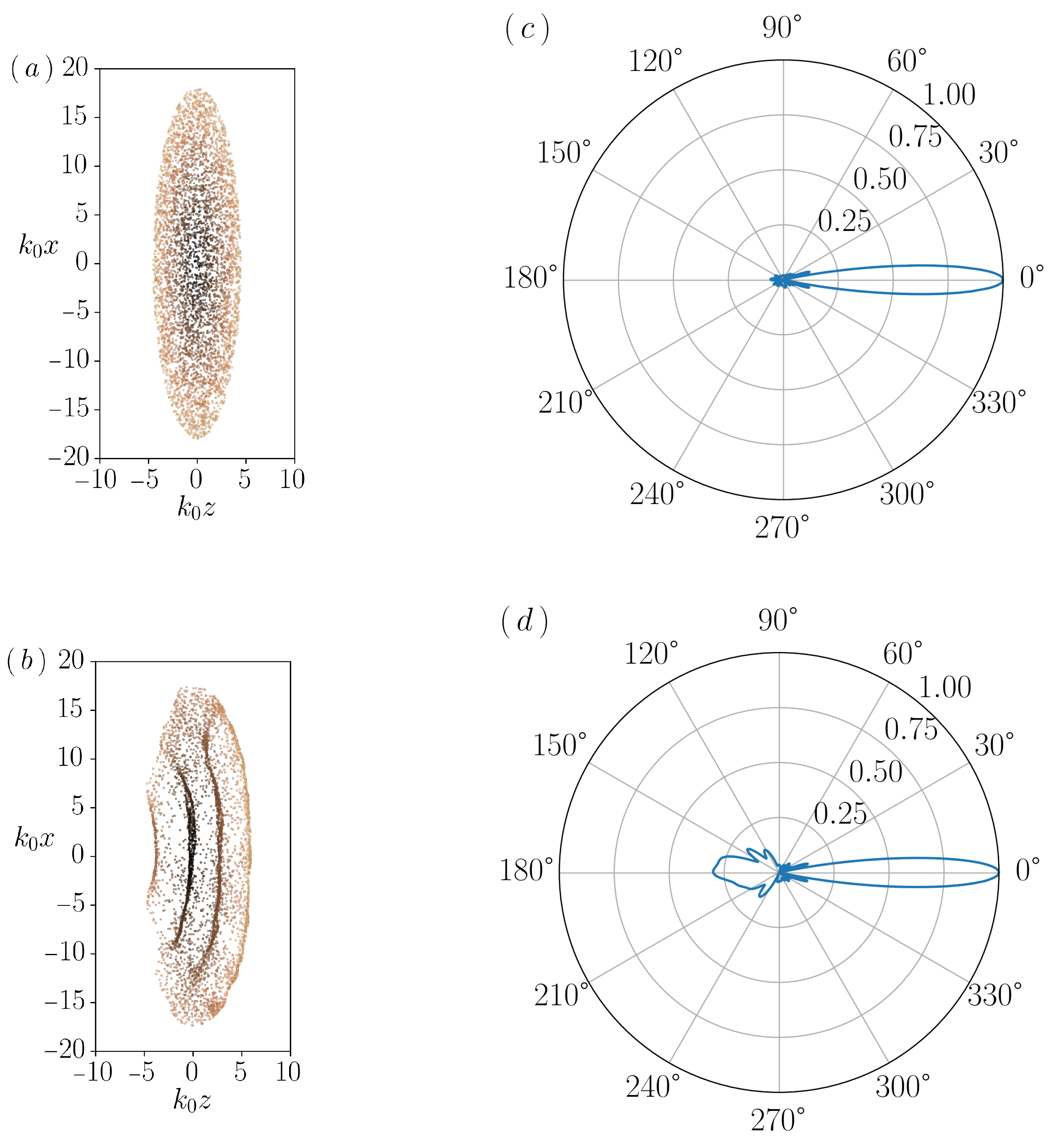
When the cloud stretches along the x axis, the atoms experiences a total momentum change of [13], i.e., depending whether the photon is emitted downward (positive sign) or upward (negative sign). When the fact that light cannot be scattered along the direction of its polarization is added to this calculated scattering event, the only possible scattering direction for the current case is the z axis. This suppresses the component of the total recoil momentum. This suppression has obvious implications both in the grating generated in the cloud and the bunching profile, due to the combined action of the external and scattered fields.
The results shown in Figure 2 exhibit remarkable changes in the grating pattern generated in the cold vapor, in comparison with the scalar case, caused by the scattering restriction imposed by the polarization vector. The polarization blocks the scattering across the transverse direction (x axis), leaving the light with the only choice but to scatter along the propagation axis of the pump field (z axis). The initial distribution, shown in panel (a), is modified into a pure 1D grating pattern depicted in plot (b) of this figure. The grating is a consequence of the two only possible atomic momentum changes: some atoms remain in place, with a net kick close to zero, while others endure a double momentum kick, with a momentum variation of .
The bunching profiles shown in the polar plot of Figure 2d is consistent with the grating patterns appearing in panel (b). The intensity pattern manifests more similarities with the one generated in the scalar case with an elliptical cloud parallel to the propagation axis, than with the analogous case that presents the same cloud orientation: only the lobes representing the forward and backwards scattering direction are visible. The backscattering lobe is somewhat distorted and not as clear as in the scalar model, although it preserves some symmetry. The main cause for a deformation of this kind may come from the dipole-dipole force which starts to push the atoms towards the right of the plot. The force pushes with greater strength the atoms located close to the origin at , where the optical thickness is larger, displacing them towards positive value of z faster than the ones located at the tips of the cloud (with larger value). Summarizing, the radiation force transforms the expected straight strips of bunches of atoms, into arcs. These are equidistantly separated with a periodic space between them of .
3.1.2. Pump Polarization Perpendicular to the Major Axis of An Elliptical Cloud: Off-Axis Scattering
We repeat the previous simulation, but now with the pump field polarization directed along the y axis. The new system does not experience any propagation restriction, because the polarization is perpendicular to the plane containing the atomic cloud. Therefore, a bi-dimensional grating similar to that obtained with the scalar model is expected to be observed for this system.
The grating portrayed in Figure 3b is not very different than the one obtained for the scalar system (see [13]). As predicted, pump polarization along the y axis does not affect the dynamics in the plane. The slight differences observed between the vectorial and scalar models arise from the short-range interaction terms. In fact, the force equation has now some additional short-range terms ( with ), and the terms that are typified in both models ( with ), are not identical. Moreover, the cut-off parameter has been augmented to , instead of the from the scalar study. The adjustment of this parameter does not affect the validity of the results, but its alteration certainly introduces a slight modification in the way particles interact with each other.
Analyzing the bunching factor in plot (d) of the same figure, it is possible to confirm that the system eventually responds as in the scalar case, providing a similar 2D pattern: two large lobes appear along the positive and negative directions of the longest scattering path (x axis). An earlier time snapshot is presented in Figure 3a,c, showing the effects of a non-negligible thickness that allows the generation of a transient 1D grating. After the preliminary formation of a longitudinal grating, the scattering direction is defined along the main axis of the ellipsoidal cloud (i.e., the x axis), hence reshaping the 1D grating into a 2D grating.
In both the simulations presented so far, we observe some atoms slowly drifting outward from the center of the ellipse. For instance, observing Figure 3, it can be identified how the cloud in (b) has expanded its area in comparison with that in (a). This is due to the ’collisions’ between the atoms: when two atoms become to close each other, the short-range terms in the force give them a kick, which is numerically controlled by the cut-off parameter, set to . To control numerically the stability of the simulation, we have assumed a cut-off parameter larger than the one adopted for the scalar case in ref. [13] (). If this value were to be applied to the present simulations with the vectorial model, the cloud would suffer a stronger and faster repulsion, making the 2D grating impossible to appear.
3.2. Scattering from 3D Cloud of a Linearly Polarized Field
3.2.1. Pump Field Perpendicular to Ellipsoid’s Major Axis with In-Plane Polarization
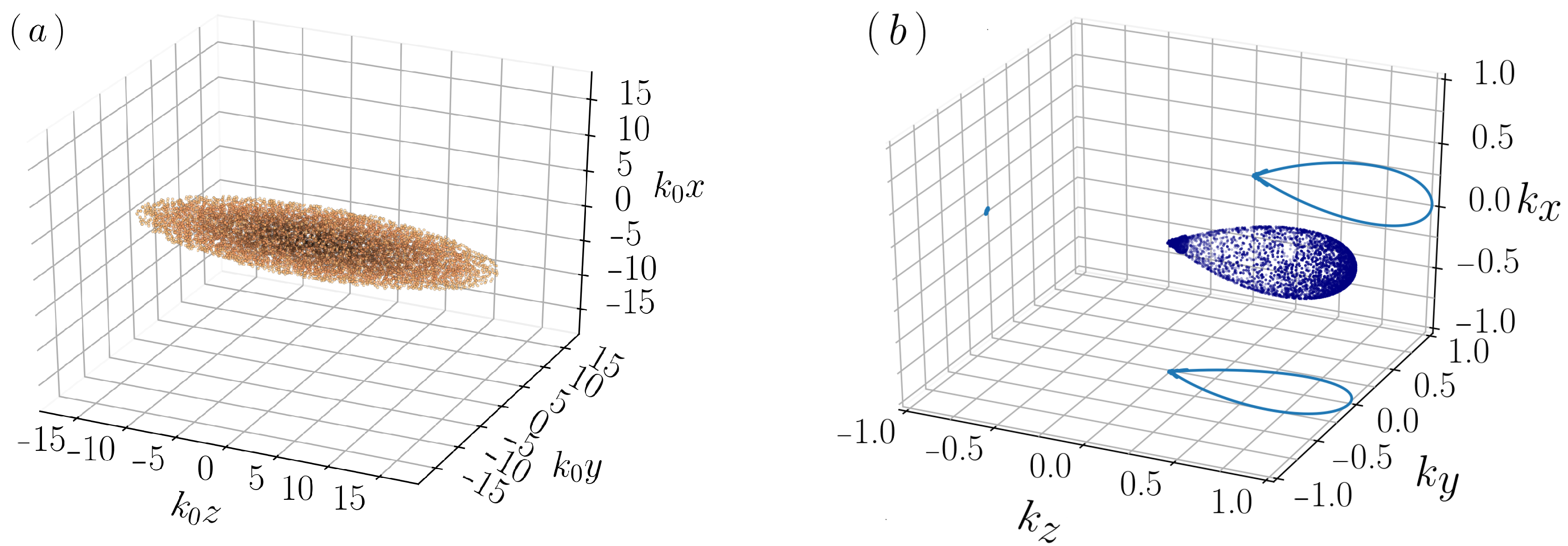
The first three-dimensional case, like in the 2D system, is investigated with the pump linearly polarized along the x axis, which forbids the scattering along that axis. Since in 3D space there are still two more propagation directions that are allowed, it is expected that the light forms a series of atomic rods (composed of several hundreds of atoms each) along the axis of the polarization vector. Again, the result is due to the combination of the photons transferred from the pump to the scattered modes along the y and z axes. Such scenario can be discerned in Figure 4b, where these atomic rods are not completely straight, displaying an arched shape, as in the 2D system, due to the effect of an electrostrictive force [13]. Since the optical thickness is larger on the central () plane (located at ), the central area endures a greater force from the pump field than the tips of the cloud, which gives to the atomic rods their characteristic arched shape. The complete suppression of the bunching along the polarization axis, can be observed in Figure 4c, where the lobes along the polarization directions (x axis) are completely missing.
3.2.2. Pump Field Perpendicular to Ellipsoid’s Major Axis with Out-of-Plane Polarization
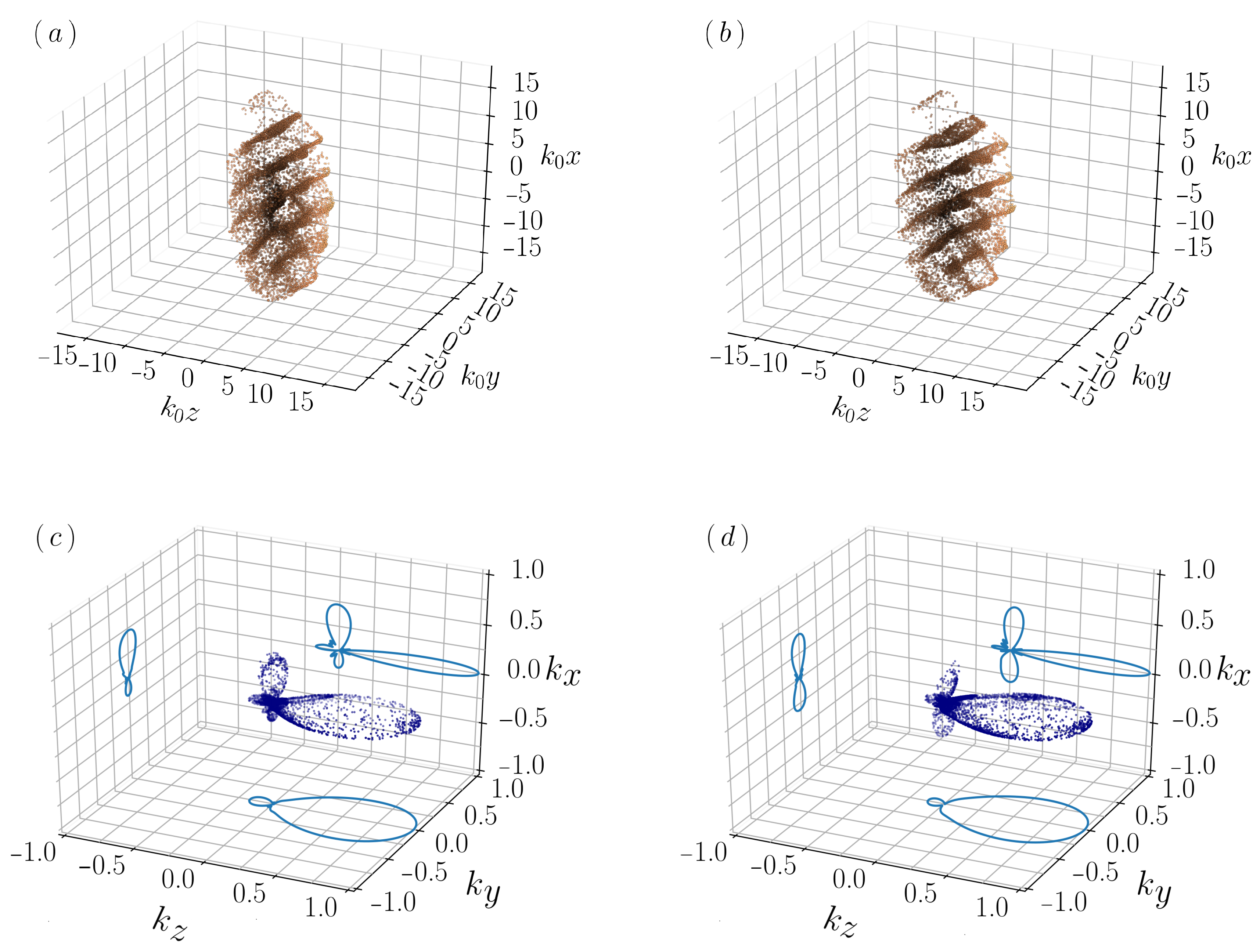
The external optical field is here considered with the polarization vector rotated with respect to the previous case, i.e., along the y axis. As the scattering is forbidden along the pump polarization y axis, tilted planes of particles are now visible in two chosen time instants: faintly drawn in Figure 5a and well defined in panel (b) of the same figure. The snapshot in (a) shows a grating composed of these tilted planes in formation. The planes with a positive slope are more visible because the atomic recoil is first directed downwards (towards negatives value of the x axis), which is confirmed by the upwards lobe of the bunching factor in panel (c). The titled planes with a negatives slope are also represented in a second snapshot (b) at a later time. Here they are dimly traced due to the latter appearance of the downwards scattering, which is represented by the downward lobe of the bunching factor in panel (d).
In addition, we do not observe any lobe in the bunching factor along the y axis either, as expected, since it is the pump polarization direction. The asymmetry observed in the lobes of bunching factor along the x-axis—see Figure 5c—is due the random initial conditions of the numerical simulations. This asymmetry is less evident at later time instant—Figure 5d—when the collective scattering process becomes dominant.
3.2.3. Pump Field Parallel to Ellipsoid’s Major Axis
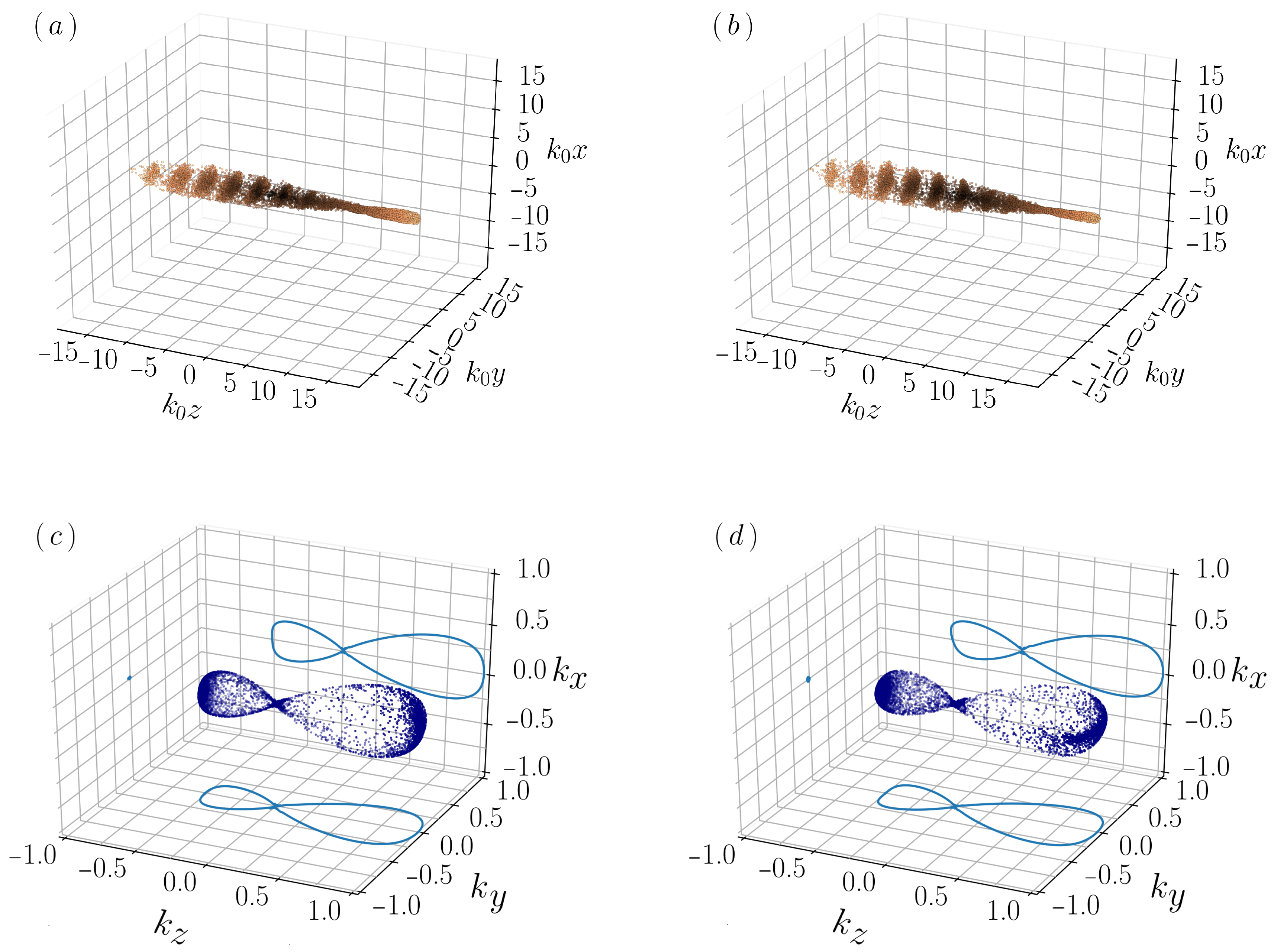
We display the pattern emerging in a characteristic “cigar-shaped” cloud of cold atoms, which elongates along the propagation axis of the pump. The cloud evolved in the presence of a linearly polarized pump field, whose initial distribution and bunching intensity profile are shown in Figure 6, is shown in Figure 7. The plots in this figure are at the same time for a cloud with same shape and initial conditions, with snapshots (a) and (c) for a pump polarized along x and snapshots (b) and (c) for a pump polarized along y.
A similar behavior than the one observed in ref. [13] with the scalar model in the 2D and 3D cases, is here seen in the bunching profile of the vectorial model. For both pump polarization cases, the bunching snapshots in Figure 7c,d show a large lobe emerging backward along the z axis (pump field axis), together with the forward lobe already present at the time in Figure 6b and due to the diffraction of the pump field [13]. The backward lobe is the well-known signature of the collective recoil lasing effect.
There are some interesting features that can be highlighted from the snapshots (a) and (b) of Figure 7. First, both panels show the cloud atomic density redistribution into a longitudinal 1D grating. Secondly, the polarization effects are visible in both the cases: the left panel shows horizontal grating due to the suppressed scattering in the vertical direction, whereas the right panel shows a vertical grating, consequence of the forbidden scattering along the horizontal direction. Lastly, both clouds undergo a squeezing effect on the radial traverse direction with respect to the z axis, stronger at the right-end of both ensembles. This electrostriction effect is a phenomenon typically observed in dielectrics, which can change their shape whenever they are subject to a strong electric field.
In the collective recoil lasing this electrostrictive effect was already observed by the scalar model in [13], with a 2D and a 3D atomic distribution. The current analysis confirms the presence of this effect with a more realistic model taking into account the light polarization. This force is not yet well understood and further investigation is needed for a satisfactory explanation. For instance, it appears that the effect rides along the cloud like a wave: it starts at the right tip of the cloud, as displayed in Figure 7a,c, and it travels backwards along the z axis. After this sort of backwards-propagating wave has passed a section, this section is not susceptible to the polarization vector of the field anymore, but it is still reactive to the gradient of the radiation force. There are some studies which have experimentally observed similar results, as the one presented in [21].
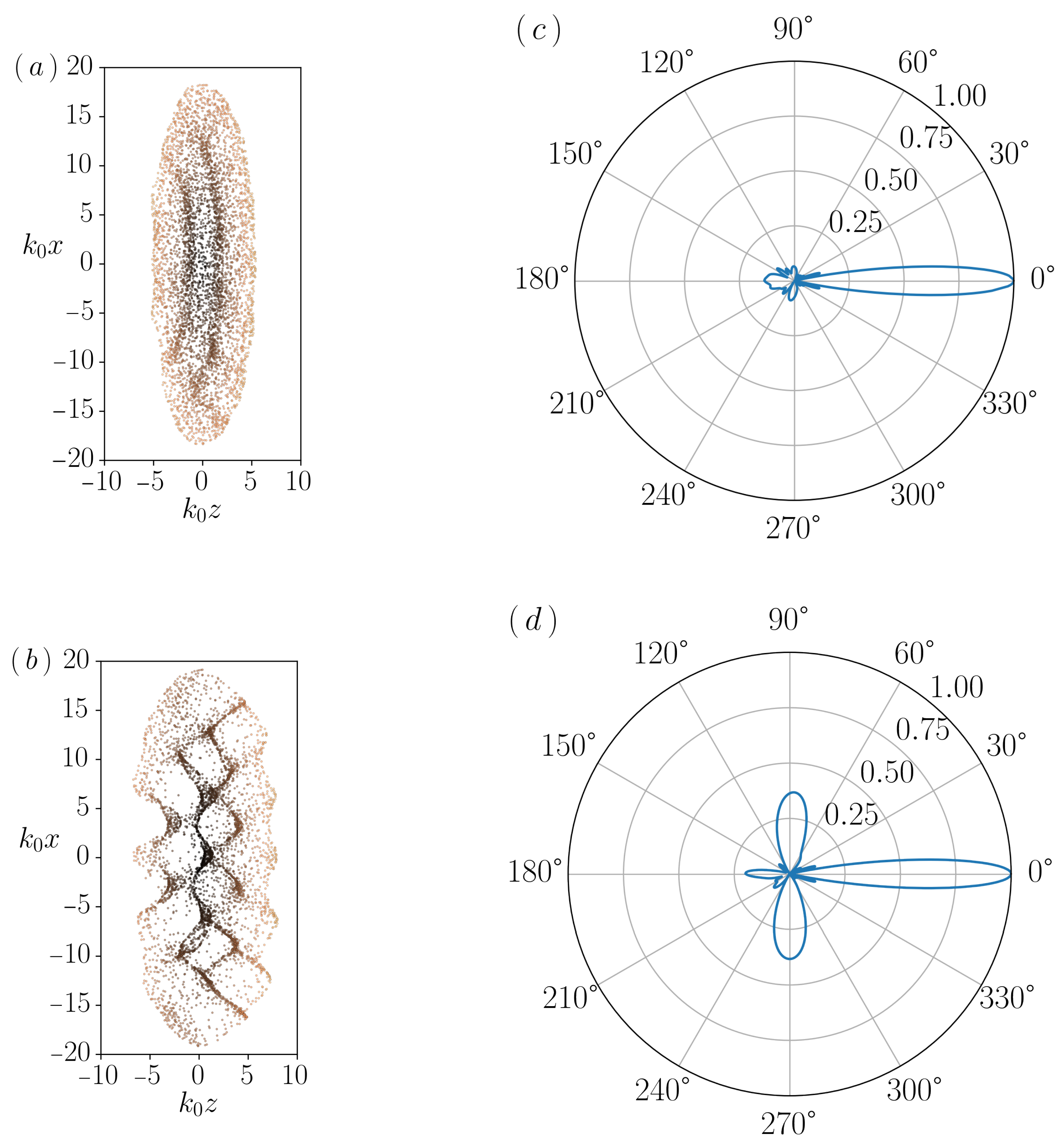
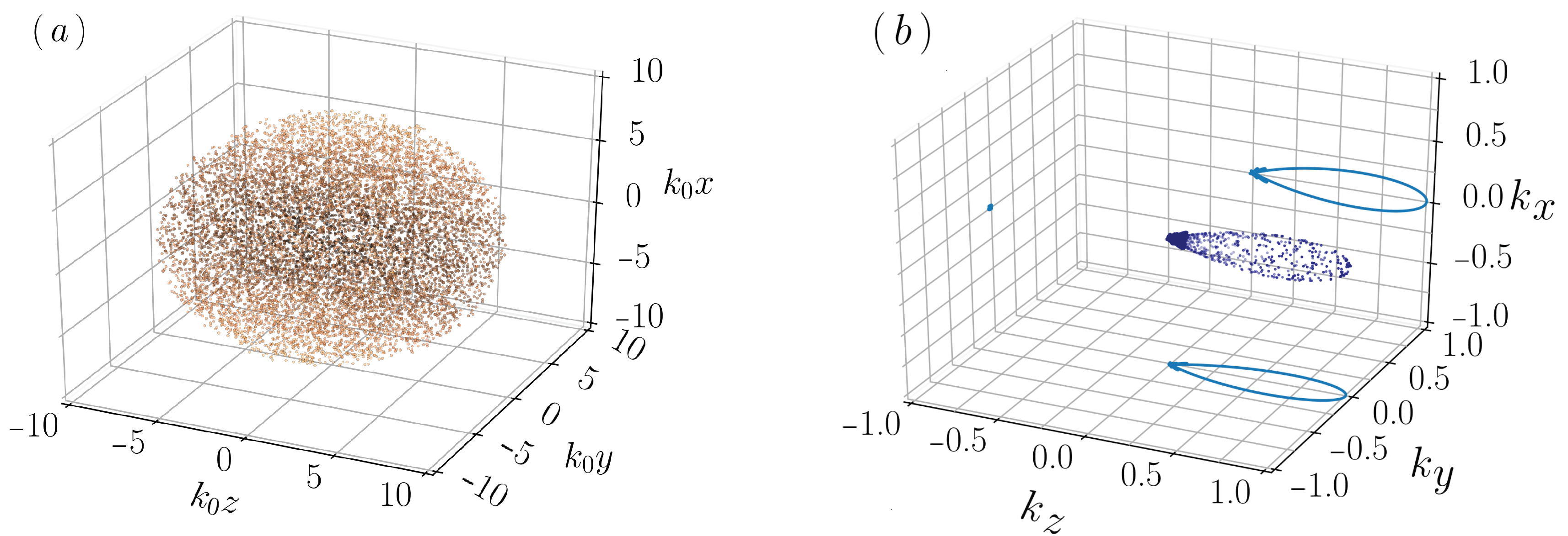
3.2.4. Scattering from a Spherical Atomic Distribution
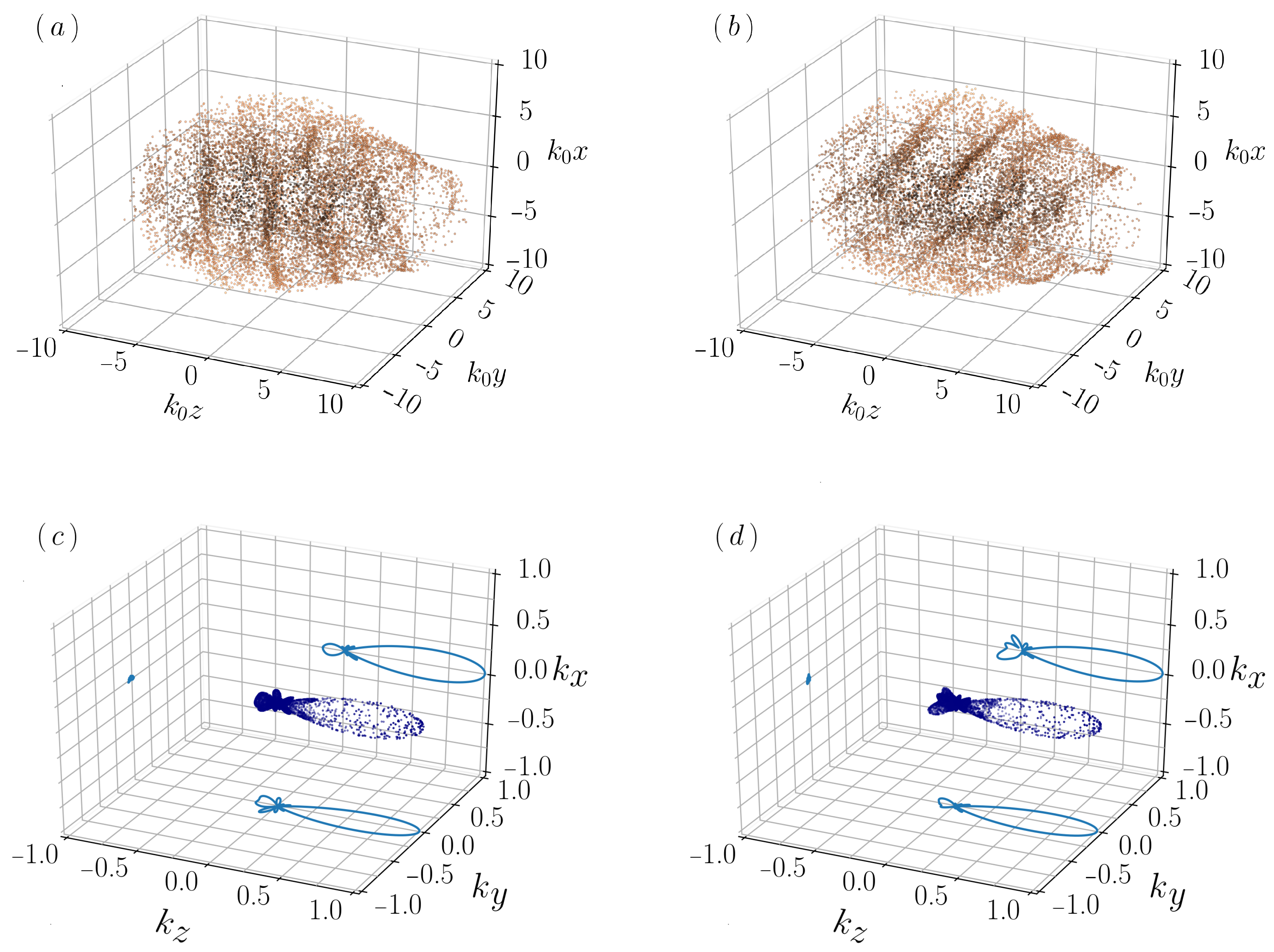
As with previous cases, a density grating also emerged when a spherical cluster of atoms is probed (see Figure 8), although no tilted planes are defined for such case. This comes because of the symmetry of the spherical initial cloud, so that no initial preferred scattering directions are present, and the atoms start to scatter randomly, except that in the direction of the polarization vector. We observed that two dynamics occurring at the same time in this case: the first one moves the inner atoms towards the shell and the outer atoms inwards; the second one distributes the particles into bunches, avoiding the polarization vector axis. On the one hand, the first action seems to be due to the electrostrictive force (outer atoms moving inwards) and the scattering effect (inner atoms moving outwards, thanks to a higher optical thickness along the z axis). The combination of these two processes deforms the edges of the cloud into an ’egg-like’ shape. In addition, this effect forces the atoms to be forward-displaced faster the closer they are to the outer shell, due to the definition of a preferred scattering path.
On the other hand, the second dynamics arises because of the photon-scattering, which starts to occur across this newly defined longest path along the external shell of the cloud. The scattering helps sketching arched rods of atoms on the outer surface vertically—Figure 9a—or horizontally—Figure 9b—oriented, depending on the polarization vector of the pump field. If the pump were to be set as a scalar field as in ref. [13], a collection of concentric circles could be spotted. However, in reality, such circles would represent the edges of shallow circular cones, which have their center located on the z axis, with a value smaller than the values of their edges.
Observing the bunching formations, in Figure 9c,d, it is possible to see that the projections onto the () plane present an elongated shape along y and x, respectively, as direct consequence of having a linearly polarized pump field. When the scalar model is used, these projections appear as a clover with four leaves, and they represent a segmentation of the spherical cloud into smaller spherical bunches of atoms following a 3D pattern.
4. Conclusions
The main scope of this work is to show the density grating formation caused by collective atomic recoil lasing, triggered in a cold atomic cloud when a polarized external optical field is applied. The results attained are similar to the ones observed with a previous scalar model [13], with the exception that when the scattering direction coincides with the polarization vector of the pump field, the scattered field is suppressed. Minor differences are seen between the patterns achieved for the scalar and the vectorial models, due to the presence of different short-range terms in either model. If the cold atomic vapor is shaped into a spherical distribution, the simulations succeed in clearly showing the electrostrictive nature of the force generated by the collective scattering process: the cloud suffers an elongation along the pump propagation axis, hence establishing the longest scattering path along the edge or the outer shell of a 2D or 3D systems, respectively. However, the experimental observation of CARL when the cold atomic vapor is shaped into a spherical distribution remains a difficult task, compared to the more favorable ellipsoidal case. Nevertheless, the role of the electrostrictive force creating some preferred direction where collective scattering set up, it is intriguing and should deserve a deeper investigation.
The present model of equations has also some numerical advantages. In fact, since the model only depends on the particles’ positions, it allows its implementation into molecular dynamics (MD) algorithm, typically employed in other scientific fields. The new open-access programming language Julia has revealed to be of great instrument to implement such MD codes, making it swift when using the built-in Julia algorithms, while allowing the accurate following of the trajectory of each particle and respecting the energy conservation of the system.
Author Contributions
All authors conceived the study. A.T.G. did the numerical simulations. N.P. directed the research. All authors contributed to writing of the manuscript. All authors have read and agreed to the published version of the manuscript.
Funding
This work was performed in the framework of the European Training Network ColOpt, which is funded by the European Union (EU) Horizon 2020 program under the Marie Sklodowska-Curie action, grant agreement 721465. R.A.
Conflicts of Interest
The authors declare no conflict of interest.
Appendix A. Derivation of the Motion Equations
Appendix A.1. Multimode Collective Recoil Equations
We consider the Hamiltonian of N two-level atoms with transition frequency and dipole d, interacting with an external field and the vacuum modes, taking into account the vectorial nature of the fields:
Here is the Rabi frequency of the laser projected along the components of the laser polarization , with electric field , wave vector and frequency with detuning . The quantum radiation modes in vacuum with wave vectors , frequencies , and polarization unit vectors are described by the operators with detuning and coupling constant , being the radiation field’s quantization volume. The internal dynamics of the atoms is described by the operators , and , where corresponds to the three degenerate excited state with magnetic number .
The coupled dynamics of the system is obtained by the Heisenberg equations for position, momentum and dipole moment operators of each atom and field operators of each mode:
where and the population of the excited state has been neglected (assuming weak field and/or large detuning ), so that and where the spontaneous decay term has been added to Equation (A4). By adiabatically eliminating the internal degree of freedom (making and substituting the resulting in the other equations) and, assuming to neglect multiple scattering effects, the equations reduce to:
where we set and , with . Equations (A6)–(A8) form the multimode CARL equations, where is summed over the polarization components. In these equations, the jth atom experiences a force which is proportional to the momentum recoil , for each mode , and to the mode amplitude .
Appendix A.2. Collective Recoil Equations in Free Space
In free space, we can also eliminate the radiation field, neglecting the re-absorption process: by integrating Equation (A8) from 0 to t and assuming the Markov approximation, the scattered field for the 3D vacuum modes due to Rayleigh scattering can be calculated as
Then, substituting the latter expression in the force Equation (A7), we obtain:
with and where we have approximated . The discrete sum over all possible modes has been transformed into an integral. The expression can be further reduced if the following relation is employed:
where . Instead of applying this relation directly to the force, it is introduced in the second integral of Equation (A10) to reduce this one. The operation is done without taking the sum of the projection of the laser polarization onto the axes and (i.e., ), because the two sums are independent from each other. Now the calculation proceeds with four steps to derive an expression that is better suited to be solve numerically.
First, the integral over is written in spherical coordinates
being and . In the integral, the z axis is chosen pointing along , so that is the polar angle of about (for simplicity, we have written instead of ).
Secondly, since the dependence on is contained only in the polarization factor , the integration over gives:
Again, for notation simplicity, is replaced by .
As a third step, a new change of integration variable, , is applied and the integral becomes:
In the fourth stage, since it can be assumed that , we replace the external field wave vector k by in every integral of the expression (everywhere except in the exponential terms) and the lower integration limit can be extended to , giving:
where is assumed. Solving the integrals over t and inserting the result into Equation (A10), a straightforward calculation leads to the following result:
where and , actually stand for and , respectively. By introducing the polarization factors
with and as the transverse components of the polarization vector of the pump, the force equation takes the following more compact form:
Appendix A.3. Radiation Field
The -component of the scattered radiation field amplitude is:
where is the ’single-photon’ electric field. Substituting the radiation field attained in Equation (A9), we obtain
As before, the relation in Equation (A11) is used to get rid of the right-most sum,
then, the integral is evaluated in polar coordinates, using once again the expression in Equation (A13):
Calculating the integrals and keeping only the term decreasing as (far-field approximation), the field can be approximated to
Afterwards, by assuming , it is viable to write , with , and the field becomes
where and is the polarization unit vector of the pump. The obtained expression is the Rayleigh scattering field in the far-field limit, i.e., a spherical radiation wave proportional to the factor form, depending on the geometrical configuration of the scattering particles [13]. Writing the field in its vectorial form, we attain:
from which the scattered intensity is
where is the angle between the scattering direction and the pump polarization , is the single-atom Rayleigh scattering intensity and
is the ‘optical magnetization’ or ‘bunching factor’. Notice that the scattering direction is determined by the bunching factor and it is suppressed if that is parallel to the pump polarization direction (i.e., if ) [22].
References
- Bonifacio, R.; Souza, L.D.S. Collective atomic recoil laser (CARL) optical gain without inversion by collective atomic recoil and self-bunching of two-level atoms. Nucl. Instrum. Methods Phys. Res. 1994, 341, 360–362. [Google Scholar] [CrossRef]
- Bonifacio, R.; Salvo, L.D.; Narducci, L.M.; D’Angelo, E.J. Exponential gain and self-bunching in a collective atomic recoil laser. Phys. Rev. A 1994, 50, 1716–1724. [Google Scholar] [CrossRef] [PubMed]
- Slama, S.; Bux, S.; Krenz, G.; Zimmermann, C.; Courteille, P.W. Superradiant Rayleigh Scattering and Collective Atomic Recoil Lasing in a Ring Cavity. Phys. Rev. Lett. 2007, 98. [Google Scholar] [CrossRef] [PubMed] [Green Version]
- Slama, S.; Krenz, G.; Bux, S.; Zimmermann, C.; Courteille, P.W. Cavity-enhanced superradiant Rayleigh scattering with ultracold and Bose-Einstein condensed atoms. Phys. Rev. A 2007, 75, 063620. [Google Scholar] [CrossRef] [Green Version]
- Inouye, S.; Chikkatur, A.P.; Stamper-Kurn, D.M.; Stenger, J.; Pritchard, D.E.; Ketterle, W. Superradiant Rayleigh Scattering from a Bose-Einstein Condensate. Science 1999, 285, 571–574. [Google Scholar] [CrossRef] [PubMed] [Green Version]
- Yoshikawa, Y.; Torii, Y.; Kuga, T. Superradiant Light Scattering from Thermal Atomic Vapors. Phys. Rev. Lett. 2005, 94, 083602. [Google Scholar] [CrossRef] [PubMed]
- Moore, M.G.; Meystre, P. Theory of Superradiant Scattering of Laser Light from Bose-Einstein Condensates. Phys. Rev. Lett. 1999, 83, 5202–5205. [Google Scholar] [CrossRef] [Green Version]
- Piovella, N.; Gatelli, M.; Bonifacio, R. Quantum effects in the collective light scattering by coherent atomic recoil in a Bose-Einstein condensate. Opt. Commun. 2001, 194, 167–173. [Google Scholar] [CrossRef] [Green Version]
- Müstecaplioğlu, O.E.; You, L. Superradiant light scattering from trapped Bose-Einstein condensates. Phys. Rev. A 2000, 62, 063615. [Google Scholar] [CrossRef] [Green Version]
- Zobay, O.; Nikolopoulos, G.M. Dynamics of matter-wave and optical fields in superradiant scattering from Bose-Einstein condensates. Phys. Rev. A 2005, 72, 041604(R). [Google Scholar] [CrossRef] [Green Version]
- Zobay, O.; Nikolopoulos, G.M. Spatial effects in superradiant Rayleigh scattering from Bose-Einstein condensates. Phys. Rev. A 2006, 73, 013620. [Google Scholar] [CrossRef] [Green Version]
- Li, J.; Zhou, X.; Yang, F.; Chen, X. Effects of including the counterrotating term and virtual photons on the eigenfunctions and eigenvalues of a scalar photon collective emission theory. Phys. Lett. A 2008, 372, 4750–4753. [Google Scholar] [CrossRef]
- Ayllon, R.; Mendonça, J.T.; Gisbert, A.T.; Piovella, N.; Robb, G.R.M. Multimode collective scattering of light in free space by a cold atomic gas. Phys. Rev. A 2019, 100, 023630. [Google Scholar] [CrossRef] [Green Version]
- Bonifacio, R.; Pellegrini, C.; Narducci, L.M. Collective instabilities and high-gain regime in a free electron laser. Opt. Commun. 1984, 50, 373–378. [Google Scholar] [CrossRef] [Green Version]
- Contributing Authors. Dynamical, Hamiltonian, and 2nd Order ODE Solvers. Available online: https://diffeq.sciml.ai/stable/solvers/dynamical_solve/ (accessed on 10 December 2020).
- Bienaimé, T.; Piovella, N.; Kaiser, R. Controlled Dicke Subradiance from a Large Cloud of Two-Level Systems. Phys. Rev. Lett. 2012, 108, 123602. [Google Scholar] [CrossRef] [PubMed] [Green Version]
- Feynman, R.; Leighton, R.; Sands, M. The Feynman Lectures on Physics; Addison-Wesley: Boston, MA, USA, 1964; Available online: https://www.feynmanlectures.caltech.edu/ (accessed on 9 December 2020).
- Hockney, R.W.; Eastwood, J.W. Computer Simulation Using Particles; Taylor & Francis: Abingdon, UK, 1988. [Google Scholar]
- Lennard-Jones, J.E. On the determination of molecular fields.—II. From the equation of state of a gas. Proc. R. Soc. A 1924, 106, 463–477. [Google Scholar] [CrossRef] [Green Version]
- Plummer, H.C. On the Problem of Distribution in Globular Star Clusters: (Plate 8.). Mon. Not. R. Astron. Soc. 1911, 71, 460–470. [Google Scholar] [CrossRef] [Green Version]
- Matzliah, N.; Edri, H.; Sinay, A.; Ozeri, R.; Davidson, N. Observation of Optomechanical Strain in a Cold Atomic Cloud. Phys. Rev. Lett. 2017, 119. [Google Scholar] [CrossRef] [PubMed] [Green Version]
- Inouye, S.; Andrews, M.R.; Stenger, J.; Miesner, H.J.; Stamper-Kurn, D.M.; Ketterle, W. Observation of Feshbach resonances in a Bose–Einstein condensate. Nature 1998, 392, 151–154. [Google Scholar] [CrossRef]
Figure 1.
Schematics describing how the leapfrog algorithm works. Position and velocity leap each other, one time and another until reaching the predefined simulation steps. The position, velocity and time are symbolized by , and , where the sub-indexes represent the time-step.
Figure 1.
Schematics describing how the leapfrog algorithm works. Position and velocity leap each other, one time and another until reaching the predefined simulation steps. The position, velocity and time are symbolized by , and , where the sub-indexes represent the time-step.

Figure 2.
Collective scattering and pattern formation from an elliptical 2D atomic cloud irradiated with a pump field propagating perpendicular to its major axis and linearly polarized along the x axis: (a) Shows the initial random atomic density distribution of . (b) Depicts the density grating formation due to collective scattering at . The corresponding bunching factors for both time instants are displayed in (c), for the initial state, and in (d), for .

Figure 3.
Collective scattering and pattern formation from an elliptical 2D atomic cloud irradiated with a pump field propagating perpendicular to its major axis and linearly polarized along the out-of-plane direction: (a) Shows the atomic density distribution of , with an initial random distribution, at the time instant . (b) Depicts the density grating formation due to collective scattering at . The corresponding bunching factors for both time instants are displayed in (c,d), respectively.

Figure 4.
Collective scattering and pattern formation from an ellipsoidal 3D atomic cloud irradiated with a pump field propagating perpendicular to its major axis and linearly polarized along the y axis: (a) Shows the initial random atomic density distribution with . (b) Depicts the density grating formation due to collective scattering at . The corresponding bunching factors for both time instants are displayed as a function of (in units) in (c), for the initial state, and in (d), for .

Figure 5.
Collective scattering and pattern formation from an ellipsoidal 3D atomic cloud irradiated with a pump field propagating perpendicular to its major axis and linearly polarized along the y axis: (a) Shows the atomic density distribution with at the time instant , with an initial random distribution. (b) Depicts the density grating formation due to collective scattering at . The corresponding bunching factors for both time instants are displayed in (c) for and in (d) for .

Figure 6.
Initial atomic distribution, in (a), and bunching factor, in (b), of an ellipsoidal 3D atomic cloud, with , irradiated with a transversely polarized pump field propagating parallel to its major axis.
Figure 6.
Initial atomic distribution, in (a), and bunching factor, in (b), of an ellipsoidal 3D atomic cloud, with , irradiated with a transversely polarized pump field propagating parallel to its major axis.

Figure 7.
Collective scattering and pattern formation from an ellipsoidal 3D atomic cloud with , with random initial positions, irradiated by a pump field propagating parallel to its major axis and linearly polarized. The snapshots at are shown for a pump polarization along the x axis, (a), and along the y axis, (b). The corresponding snapshots of the bunching factors are shown in (c,d).

Figure 8.
Initial atomic distribution, in (a), and bunching factor, in (b), of a spherical 3D atomic cloud, with , irradiated with a transversely polarized pump field propagating parallel to its major axis.
Figure 8.
Initial atomic distribution, in (a), and bunching factor, in (b), of a spherical 3D atomic cloud, with , irradiated with a transversely polarized pump field propagating parallel to its major axis.

Figure 9.
Collective scattering and pattern formation from a 3D spherical atomic cloud with , with random initial positions, irradiated by a pump field linearly polarized. The outcome for the polarization along the x axis is portrayed in (a), whereas the ones for the polarization along the y axis is illustrated in (b). In both systems the density grating formation due to collective scattering is pictured at . The corresponding bunching factors for both systems, are respectively displayed in (c,d).

Publisher’s Note: MDPI stays neutral with regard to jurisdictional claims in published maps and institutional affiliations. |
© 2020 by the authors. Licensee MDPI, Basel, Switzerland. This article is an open access article distributed under the terms and conditions of the Creative Commons Attribution (CC BY) license (http://creativecommons.org/licenses/by/4.0/).
Share and Cite
MDPI and ACS Style
Gisbert, A.T.; Piovella, N. Multimode Collective Atomic Recoil Lasing in Free Space. Atoms 2020, 8, 93. https://0-doi-org.brum.beds.ac.uk/10.3390/atoms8040093
AMA Style
Gisbert AT, Piovella N. Multimode Collective Atomic Recoil Lasing in Free Space. Atoms. 2020; 8(4):93. https://0-doi-org.brum.beds.ac.uk/10.3390/atoms8040093
Chicago/Turabian StyleGisbert, Angel T., and Nicola Piovella. 2020. "Multimode Collective Atomic Recoil Lasing in Free Space" Atoms 8, no. 4: 93. https://0-doi-org.brum.beds.ac.uk/10.3390/atoms8040093
Note that from the first issue of 2016, this journal uses article numbers instead of page numbers. See further details here.