1. Introduction
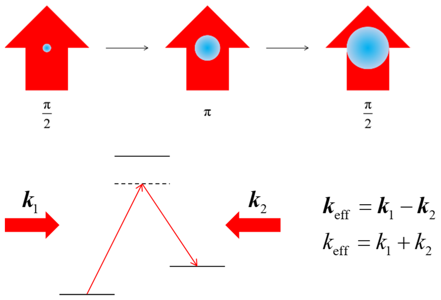
Atom interferometry offers the potential to deliver high-performance, compact, and robust gyroscopes that are suitable for inertial navigation applications. Critical requirements for such an atomic gyroscope include a high sensitivity to rotations and the ability to distinguish between signals arising from rotations and accelerations. Here, we describe a multi-axes gyroscope based on the combination of point source interferometry (PSI) [
1,
2,
3] and large momentum transfer (LMT) beam splitters [
4,
5] which are well-suited to meet these requirements. In a PSI, Raman pulses are applied during the expansion of a point source of atoms. The pulses are a pair of counter-propagating laser beams that drive two-photon Raman transitions [
6], serving as the beam splitters and mirrors for a Mach–Zehnder light-pulse atom interferometer [
7,
8,
9,
10,
11,
12,
13], as shown in
Figure 1. The interferometer phase response to rotation scales linearly with the velocity difference of the atoms in the two arms, while the response to acceleration is independent of the atomic velocity. Because of this difference, the signal in a PSI allows rotation and acceleration to be distinguished. The PSI can also determine both components of the rotation vector that are orthogonal to the laser pulses, thus realizing a multi-axes gyroscope. It should be noted that there are other techniques that can also distinguish between rotation and acceleration [
9,
10,
11,
12,
13]. However, a key practical advantage of the PSI is that it only requires a single atom cloud and Raman beams along a single axis, in contrast to other methods.
The LMT beam splitters we consider involve the use of tailored laser pulse sequences to increase the momentum splitting, and therefore the velocity difference, between the two arms of the interferometer. Via the Sagnac effect, the rotation sensitivity of a gyroscope is proportional to the area enclosed by an interferometer. The enclosed area is proportional to the velocity difference induced by the beam splitter; as such, the rotation sensitivity scales linearly with the momentum transferred by the laser pulses during the beam splitting process.
The conventional model of the light-pulse interferometer as well as the PSI makes the approximation that each atom has a well-defined velocity as well as a well-defined position. This model is apparently inadequate for describing the behavior of a PSI accurately for several reasons. The first is that the wave packets of cold atoms cover large spatial extents and thus do not have trajectories that enclose a well-defined area. The second is that atoms are in superpositions of many momentum eigenstates, with each of them seeing a different light frequency. Yet the model has proven to be quite useful in predicting the behavior of a light-pulse interferometer as well as the PSI in most circumstances of experimental relevance. As such, in the initial stage of our analysis, some of the salient features of the effect of large momentum transfer on the PSI are extracted from the conventional model. Later on, we augment the analysis with a more rigorous model wherein the center of mass motion of each atom is treated quantum mechanically, represented as a superposition of plane waves, since it is not a priori obvious, without experimental results, whether the semiclassical model would be adequate when the PSI is augmented by large momentum transfer.
The rest of the paper is organized as follows. In
Section 2, we use the conventional model to summarize first the basic properties of a PSI without large momentum transfer (LMT). We then use the same model to determine how the signal for a PSI would be modified in the presence of LMT, without taking into account non-idealities such as Doppler detuning and spontaneous emission. We also describe how the signal for an LMT–PSI is modified when the point source is replaced by a source with a finite extent and determine how the enhancement in sensitivity varies as function of the degree of momentum transfer under the LMT process, as well as the initial size of the source. In
Section 3, we present the augmented quantum model where the center mass motion of the atom is treated quantum mechanically. We consider first the ideal case where an atom is in a pure state. This is followed by a consideration of a situation where the atoms are thermalized in a harmonic oscillator potential before being released for the LMT–PSI process, taking into account quantum statistics. We conclude this section with a discussion of how the results of this augmented quantum model compare with those of the conventional semi-classical model under various conditions. Specifically, we find that for thermal atoms, the predictions of these two models do not differ significantly. In
Section 4, we analyze the combined effect of all non-idealities, including Doppler detuning, spontaneous emission, and the finite size of the source, using the augmented quantum model. However, in order to be able to carry out an analytical estimation of the enhancement in sensitivity expected for a significant degree of LMT, we make some simplifying assumptions that render the model essentially equivalent to that of the conventional semi-classical model. We expect that a full-blown version of the augmented quantum model would produce results that agree closely with the conclusions reached in this section. But such a full-blown analysis requires enormous computational resources; given that the difference between the results produced by the semi-classical analysis and the augmented quantum model is very small, undertaking such an analysis was not deemed critically important at this point. Instead, it is expected, subject to experimental verification, that the predictions of the effectively semi-classical model would be adequate. Finally, we summarize the results in
Section 5.
2. Conventional Model
As noted above, the conventional model of a PSI makes the approximation that each atom has a well-defined velocity as well as a well-defined position. Therefore, the atoms follow definitive trajectories that enclose an area. Specifically, the enclosed area is
, where
is the differential momentum transferred to an atom from the initial light pulse,
is the displacement of the atoms,
is half of the total time elapsed, from splitting to recombination, and
is the mass of each atom [
14]. The Sagnac phase shift is proportional to the enclosed area according to the expression
, where
is the Compton frequency of each atom [
15], and
is the angular velocity of the rotation. It then follows that the phase shift can be expressed as
. The measured signal is the spatial distribution of the ground state population, given by the expectation value of the projection operator
. As such, the signal can be expressed [
8] as
, which is a pattern of spatial fringes dictated by the wave number
, multiplied by
, the final profile of the atomic cloud. With this model, it seems obvious that by increasing
, we can increase
, thus reducing the fringe spacing, and thereby increasing the sensitivity of the PSI.
To determine quantitatively the density of fringes, we have to compute the Fourier transform of the pattern. Experimentally, this Fourier transform can be observed in real time using a lens in the system for imaging the atom cloud. Thus, our signal is expressed as
, where
is the position space projection operator for atoms in the ground state, as defined earlier. It should be noted that
is different from
, the momentum space projection operator for atoms in the ground state. The semi-classical model gives a signal that can be expressed as:
where
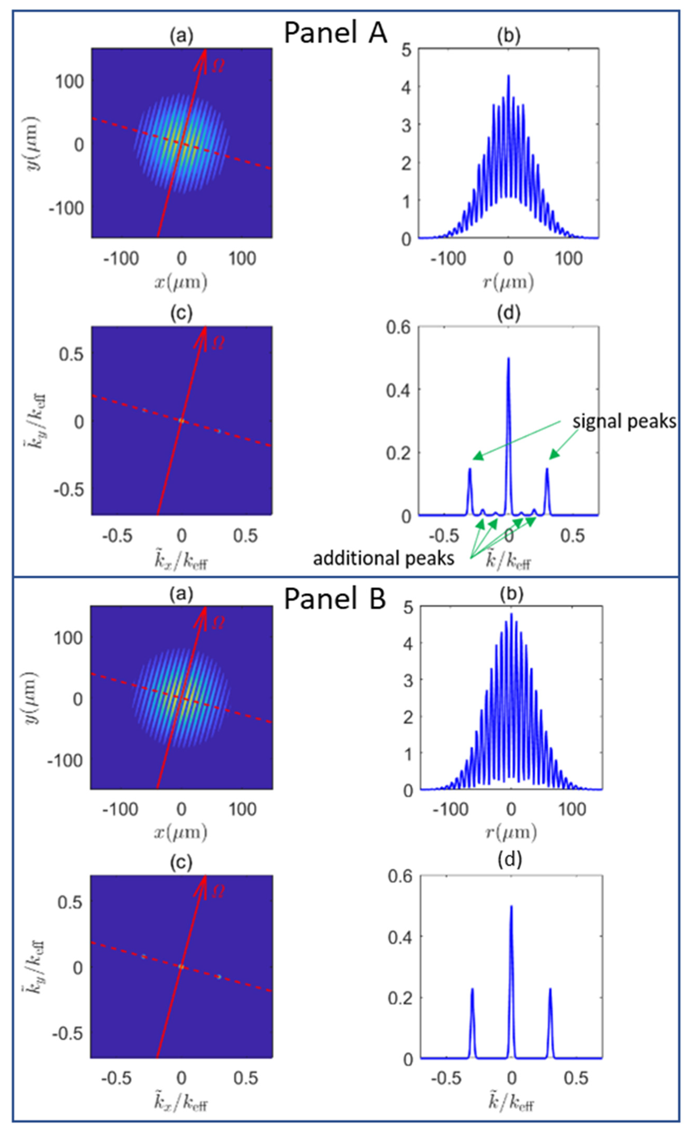
is the Fourier transform of the profile of the atomic cloud. The spatial fringes representing
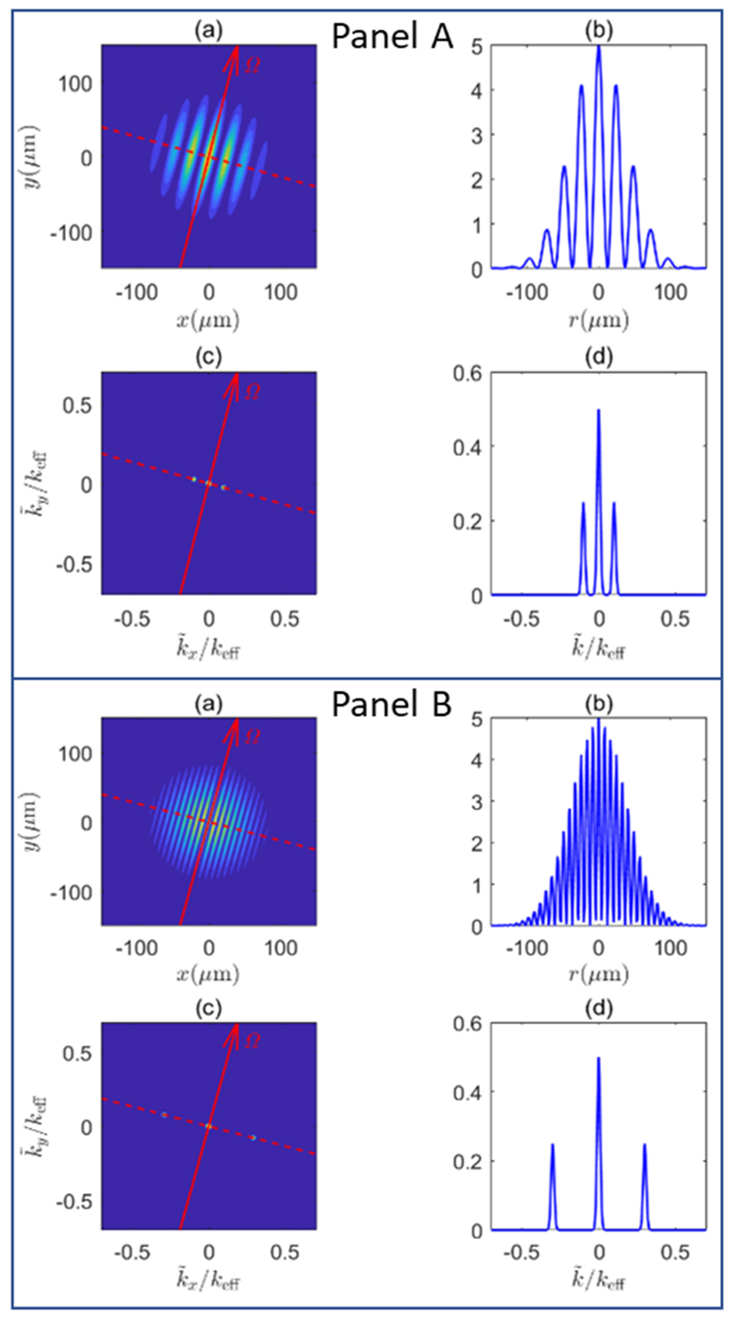
and the corresponding Fourier transforms given by
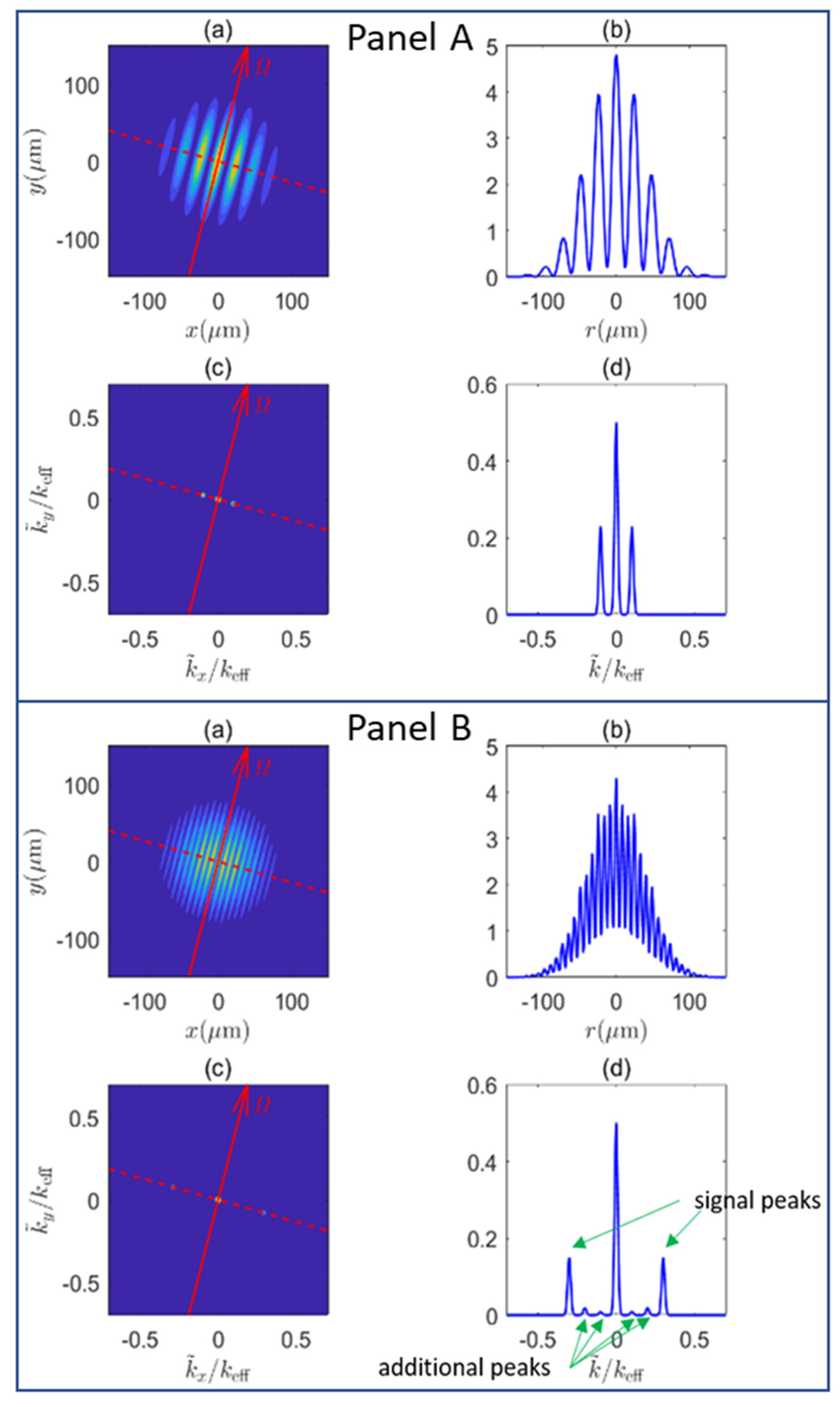
derived from the semi-classical model are depicted in
Figure 2. Panel A shows plots for
and panel B shows plots for
. In each panel, (a) is the plot of
, with
, in the plane perpendicular to
, (b) is the cross section at the dashed line in (a), (c) is the plot of
in the plane perpendicular to
, and (d) is the cross section at the dashed line of (c). In the Fourier domain, the distance from a signal peak, for example,
, to the central peak
, is
, which is proportional to the angular velocity we want to measure. The height of the signal peak
corresponds to the contrast of the fringes, and ideally
.
In this model, for an ideal point source, the final position of an atom is determined by its initial velocity. The velocity spread of the atoms is given by the Boltzmann distribution characterized by the temperature of the atomic cloud. Therefore, the final population distribution of the atoms has a three-dimensional Gaussian profile,
, where
describes the final size of the atomic cloud, determined by the initial velocity spread and the expansion time. Thus, the final spatial distribution of the ground state atoms can be expressed as
. In the plots shown in
Figure 2, we assumed such a Gaussian envelope for the ground state populations, with an arbitrarily chosen value of
. Here,
Figure 2a in each panel is simply a plot of this expression for
.
This model can also be used to analyze the effect of the finite size of the initial atomic cloud. For this analysis, we assumed that the Raman pulses were along the z-direction, while the angular velocity vector was in the y-direction. Then the interference fringes were oriented in the x-direction. For simplicity, we looked at a slice of the atomic cloud in the x-direction, for
y =
z = 0. The population in this slice can be expressed as
. The initial cloud of a finite size is a collection of the many ideal point sources. We assumed the initial distribution of the atomic cloud to be of the form
. The final spatial distribution of the ground state atoms is then the convolution of
and
:
It is easy to see that
has the form of
where [
2]
Equation (3) implies that the signal peak is at a distance away from the central peak in the Fourier transform domain. Thus, if the point source has a finite size, the signal peak moves closer to the central peak and the height of the signal peak is reduced. The uncertainty in the position of the signal peak in turn determines the uncertainty in the determination of . Specifically, from the expression of stated earlier, and assuming that is orthogonal to , it follows from Equation (3) that . In general, the uncertainty of a signal is the linewidth divided by the signal-to-noise ratio. Using this rule, we can write that , where is the width of the signal peak and is a constant coefficient. It then follows that . Since the signal is in the Fourier transform domain, is approximately the inverse of the final size of the atomic cloud. Therefore, is determined primarily by the free expansion and is not affected significantly by the LMT process. Thus, we see that the larger the final atomic cloud size is, the smaller is, and the smaller is. This reduction in can be understood physically by noting first that the width (i.e., ) of each of the peaks in the Fourier Transform domain becomes smaller for larger final atomic clouds. Since the uncertainty in the measured value of the rotation rate is proportional to this width, it then follows that a larger final atomic cloud yields a smaller value of .
To compare LMT–PSI’s with different values of
, we assumed that the atomic clouds ended up with the same final size, and therefore the same
, independent of the value of
N. We defined an improvement parameter
. In experiments, the final size of the atomic cloud is determined by the size of the apparatus, and thus can be considered a rigid constraint. For concreteness, we assumed the value of
to be 1 cm. We also assumed the initial temperature to be 6 μK, a value that can be achieved typically with optical molasses [
2]. The expansion time is related to the initial and final sizes of the atomic cloud according to the expression
. In
Figure 3, we show a plot of the improvement factor versus the momentum transfer, with two different initial sizes of the atomic cloud and two angular velocities. The red curves are the plots for
while the blue curves are for
. The solid (dashed) curves correspond to an angular velocity of 1 (2) µHz. We can see that LMT can improve the PSI more for smaller initial atomic clouds and for measuring a smaller angular velocity.
As noted earlier, even though the semi-classical model has been highly accurate in predicting the behavior of a light-pulse interferometer as well as a PSI, it is potentially useful to employ a more rigorous model that treats the center of mass motion of each atom quantum mechanically [
16], since it is not evident a priori whether the semi-classical model would lead to correct predictions of observables when the point source interferometer is augmented by large momentum transfer. As such, in what follows, we present such a quantized model to augment the description of the LMT–PSI.
3. Augmented Quantum Model
The quantum state of an atom consists of its internal state and the state of its center of mass. Each atom in a PSI starts with its internal state as the ground state
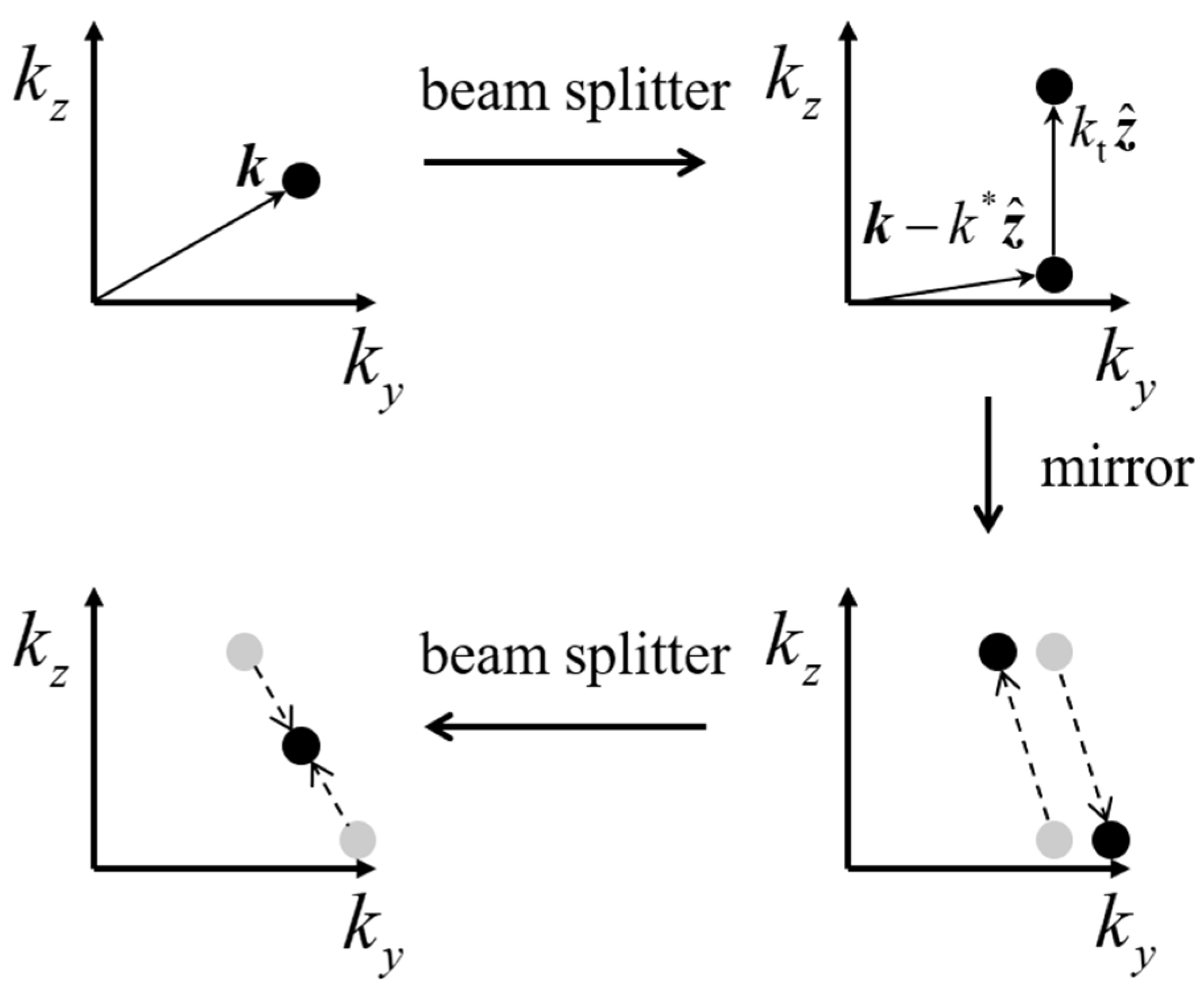
. We first considered the case where the center of mass of the atom is initially in a momentum eigenstate
. The evolution of the state of the center of mass is illustrated in
Figure 4. The first atomic beam splitter propagating in the
z-direction splits the atom into a superposition of the state
and the state
. Here,
is the difference in the momentum between the two arms, and
is the common shift in the momentum for each arm. The value of
is zero for a conventional light-pulse atom interferometer but it has a non-zero value when the technique of LMT is employed. The value of both
and
depend on the details of the LMT process. For simplicity, we worked in a picture where the energy of the state
and the state
were the same and defined as zero. The atomic mirror pulse is applied at a time
after the first atomic beam splitter. Due to the rotation perpendicular to the
z-direction, the atomic mirror pulses are no longer in the original
z-direction, but at an angle
with respect to it. We assumed that the angular velocity of the rotation was in the
x-direction, without loss of generality. For
, the atomic mirror pulses turn each atom into a superposition of the state
and the state
. The last atomic beam splitter will combine these two states approximately back to the point
in the momentum space. The Sagnac phase shift can be viewed as arising from the energy difference between the states
and
. To see this, note first that the energies of these two states are no longer zero, but
. Therefore, these two states oscillate at frequencies that have a difference of
. The Sagnac phase shift is the product of this frequency difference and
, the duration for the second half of the interferometry process:
. It can also be written as
, where
. Note that
, and while it has the dimension of distance, it does not represent the spatial coordinates of the center of mass of the atom. It can be shown that this expression of the phase shift is equivalent to the phase shift under the conventional description if we assign to a momentum eigenstate
a localized state with a velocity of
, determine the vectorial area
enclosed by the resulting trajectories, and use the expression
.
Due to the rotation induced phase shift, the population of the ground state will be , where is the momentum space projection operator for atoms in the ground state, defined earlier. Consequently, if initially the atoms have a continuous distribution in the momentum space, the final distribution of the ground state population will form fringes in the momentum space. Next, we will discuss what the fringes in the momentum space mean in the coordinate space.
Here, we considered both the cases where the atoms are in a pure state and in a mixed state. If the atoms are in a pure state, then the external motion can be described by a wavefunction
for each atom. In the absence of rotation, the final external state of the atom internally in the ground state will be
. According to the preceding discussion, in the presence of rotation, the final external state of the atom internally in the ground state will be:
Rearranging Equation (5) and eliminating the common phase factor, we can write:
where
. To find the wavefunction of the atoms in the coordinate space, we computed the Fourier transform of
, to obtain:
where
stands for Fourier transform. The spatial distribution of the ground state
for an arbitrary
has to be calculated individually.
However, under the condition where the width of is much larger than so that , both and will approximately equal , which is just the final external state of the atom internally in the ground state in the absence of rotation, as discussed before Equation (5). In that case, is simply the product of the final profile of the atom cloud and a sinusoidal function . This is exactly the result predicted by the conventional model for a point source.
The condition , corresponding to a smaller difference between and , yields the highest contrast in the spatial interference fringes. A state wider in the momentum space corresponds to a smaller difference between and . This condition also corresponds to a state narrower in the position space. Therefore, for a pure state, the narrower it is in the position space, the higher the contrast is for the spatial fringes. The limiting case of narrow wavefunctions in the position space is, of course, the point source.
However, the centers of mass of all trapped atoms cannot generally be described as a pure state. According to quantum statistical mechanics, the state of the center of mass of each atom can be described by a density operator
, where
is the Hamiltonian,
is the Boltzmann constant, and
is the temperature. If we assume the atoms to be non-interacting and freely moving, we have
, so that the state of the center of mass of each atom is described by a density operator
. This density operator lacks coherence between different momentum eigenstates because these are also the eigenstates of energy. For such a system, there will be no spatial fringes at all. To see why, we recall that, for a pure state, the width in the
space determines the contrast of the spatial interference fringes. Every pure state in the density operator
has no width in the
space. Consequently, no spatial fringe will appear. The existence of coherence between different
states for atoms cooled by lasers have been demonstrated in experiments [
17,
18,
19]. Therefore, the diagonal density matrix is inadequate, and we need a different model to describe the initial state of such cold atoms.
We considered a situation where the atoms released from a magneto-optic trap are caught in an isotropic dipole force trap before the onset of the PSI process. Such a trap can be modeled as a harmonic potential well [
20] with a characteristic frequency
ω, so that the Hamiltonian can be expressed as:
The energy eigenstates of this Hamiltonian are:
where
is a measure of the size of the trap and
is the
n-th order Hermite polynomial. The density operator of the atoms in this case can be expressed as:
During the expansion of the atom cloud, upon release from the trap, each
(defined as the state where the external state is
and the internal state is
) evolves independently. The evolution of each
under the sequence of pulses used for the PSI can also be evaluated individually. We defined as
the final external state corresponding to
, for an atom in the ground state internally. The signal at the end of the PSI process can thus be expressed as:
where
is the momentum space projection operator for atoms in the ground state, as defined earlier. Equation (11) shows that the overall contrast is determined by the sum of the fringes resulting from each energy eigenstate,
. Therefore, the smaller
a is, the narrower all the energy eigenstates will be in the position space, and the higher the contrast of the spatial fringes will be.
In
Figure 5, we show a comparison between the signal of the PSI for two different values of
a. For simplicity, we have considered here the case where the rotation is around the
y-axis only, so that fringes occur only in the x-direction. For both curves, the temperature of the atoms was
, and the half expansion time
. The rotation rate wavenumber used was
. The red curve shows the case where
a = 0.002 cm, and the blue curve shows the case where
a = 0.004 cm. We can see that with a smaller
a, the contrast of the interference fringes was higher, as expected. In the simulation, we assumed that the sum in Equation (11) was truncated at a maximum occupation number,
nmax, for the harmonic oscillator. This occupation number is dictated by the parameter
. Specifically, the sum in Equation (11) was carried out from
n = 0 to
nmax = 4
α and rounded to the nearest integer, which is sufficient to ensure that contributions from the excluded terms (i.e., for terms with
n > 4
α) were negligible. For the red curve, we had
α = 7.2 and for the blue curve
α = 28.9.
To show the relationship between the augmented quantum model and the semi-classical model, we considered the artificial case of a one-dimensional harmonic oscillator along the x direction. The starting point was the density of atoms along the x-direction at the onset of the PSI process. Since all the atoms were assumed to be in the ground internal state, this density distribution for the augmented quantum model can be determined from the density operator in Equation (10) as follows:
where
is the projection operator for atoms in the ground state, and
is the Hermite–Gaussian spatial wavefunction for the
n-th eigenstate of the harmonic oscillator. The corresponding density distribution according to the semi-classical model and classical statistical mechanics can be expressed as:
It then follows that the initial cloud size parameter in the semi-classical model is related to according to the expression . We recalled that the harmonic oscillator scale parameter a in the augmented quantum model was related to according to the expression . Thus, we see that . At a first glance, it may not at all be obvious how the augmented quantum model density distribution as given by Equation (12) is related to the semi-classical density distribution as given by Equation (13). However, it turns out that for a highly thermal case, corresponding to , these two distributions are essentially identical. This is not surprising, since a highly thermal system generally behaves in a manner similar to what is expected classically.
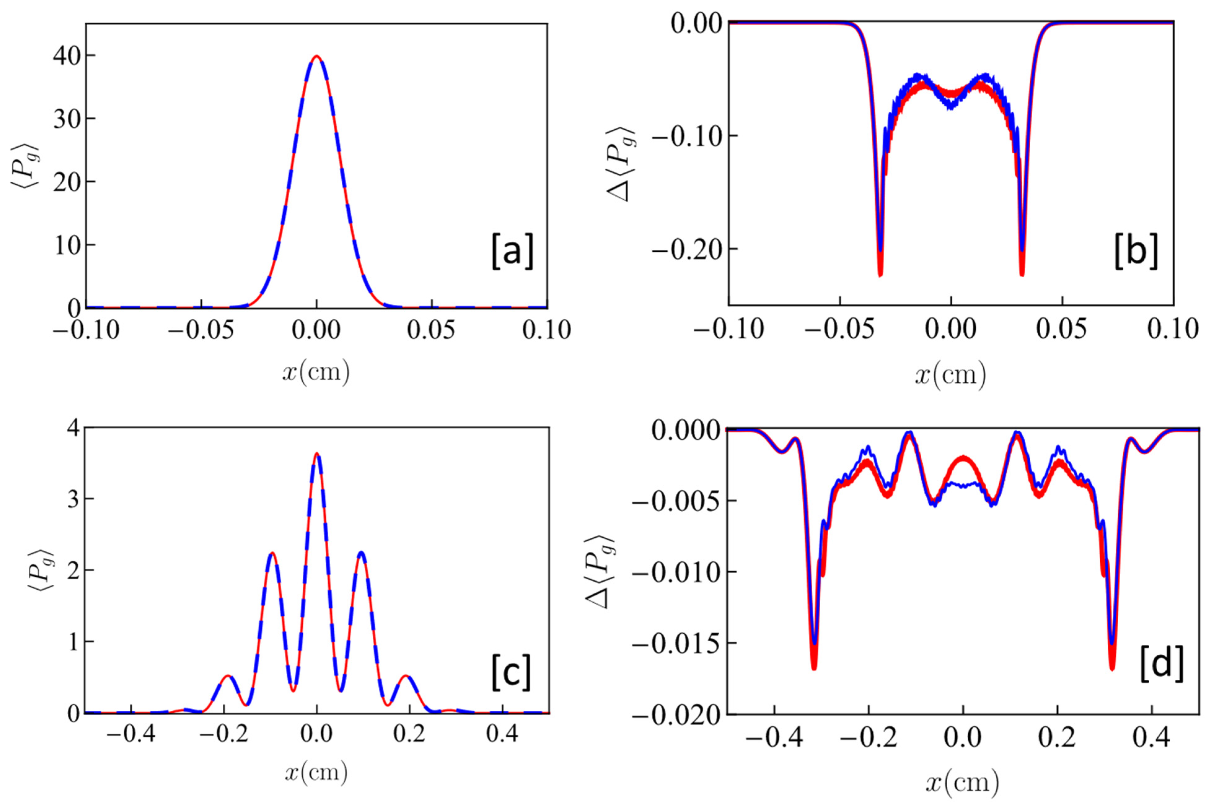
We illustrate this correspondence in the top panel of
Figure 6. In
Figure 6a, we show plots of this density distribution using the expressions from both the augmented quantum model (red) of Equation (12) and the semi-classical model (dashed blue) of Equation (13). The parameters used were
,
α = 10 and
nmax = 40. The plots are almost identical, and the difference is hard to infer from these plots. As such, in
Figure 6b, we have shown in the blue curve the difference between the density distribution for the augmented quantum model and the semi-classical model for the plots shown in
Figure 6a. In the red curve in
Figure 6b, we have shown the corresponding difference when
α = 20 and
nmax = 80, with the value of
unchanged. Thus, we see that this difference, while small, is real, and did not tend to vanish as the value of
α increased.
Next, we considered the PSI interaction. The fringes produced by the augmented quantum model (red) and the semi-classical model (dashed blue) are shown in
Figure 6c. The parameters used here were
,
,
α = 10,
nmax = 40, and
. Again, the plots are almost identical, and the difference is hard to infer from these plots. As such, in
Figure 6d, we have shown in the blue curve the difference between the density distribution for the augmented quantum model and the semi-classical model for the plots shown in
Figure 6c. In the red curve in
Figure 6d, we have shown the corresponding difference when
α = 20 and
nmax = 80, with the value of
and
unchanged. Again, we see that the difference, while small, is real, and does not tend to vanish as the value of
α is increased.
We recall that, according to the Ehrenfest theorem, the behavior of the quantum mechanical expectation values of the position and the momentum of a particle are identical to their classical values if the Hamiltonian is at most quadratic in position as well as momentum. The condition for the Ehrenfest theorem is satisfied for free space propagation, as well as the Sagnac effect, which is modeled here as a simple rotation in the coordinate system. On the other hand, the Hamiltonian representing the interaction with the light fields for the PSI considered in
Figure 6, has a spatial dependence of the form
, which is not consistent with the requirement of the Ehrenfest theorem. However, in the semi-classical model, the effect of such a Hamiltonian is considered
quantum mechanically (rather than classically), in assigning a momentum difference of
between the two arms. As such, it is reasonable to conclude that the difference in the signals for the PSI computed by these two models differ due to the difference in the initial density distributions only.
To summarize, for highly thermal atoms
released from a harmonic oscillator trap, the PSI signals predicted by the augmented quantum model would be very similar to, although not exactly the same as, those predicted by the semi-classical model. However, if
, this convergence of results will not occur. The extreme example is the Bose-Einstein Condensate (BEC). The pure case considered above in fact corresponds to the BEC (with the order parameter behaving as the single particle wavefunction) in the ideal limit where the scattering length vanishes and there is no interaction among the atoms [
21]. As we have shown above, the PSI signal in that case would be the same as that predicted for an ideal, point-source based PSI employing the semi-classical model, but only in the limit where the initial momentum spread is much larger than
. For the realistic cases where the scattering length does not vanish, the augmented quantum model would be more complicated due to non-linearity; such an analysis is beyond the scope of this paper. Furthermore, it is not clear whether there is an effective semi-classical model for a BEC, especially in this non-linear regime.
4. Large Momentum Transfer by Additional Raman Pulses
Large momentum transfer (LMT) atom optics are broadly defined as methods that increase the momentum splitting between the interferometer arms beyond 2ħk. In light-pulse atom interferometry, several LMT techniques have been demonstrated. These include using an additional sequence of π pulses [
4,
5,
22,
23,
24,
25,
26] or Bloch oscillations in an optical lattice [
27,
28,
29,
30] following the initial π/2 pulse to increase the momentum splitting, as well as implementing individual π/2 pulses that transfer an increased number of photon momentum recoils via higher order Bragg diffraction [
31]. For the sequential pulse method, either Raman transitions [
15], which change the internal hyperfine state, or Bragg transitions [
4,
5,
18,
19], which leave the internal state unchanged, can be used. Both methods have their advantages and are worth considering for a given application. For instance, Raman transitions are capable of efficiently transferring atom clouds with wider velocity spreads along the laser beam axis [
23], while Bragg transitions are immune to sources of noise or drift arising from effects involving a changing internal state, such as ac Stark shifts of the transition resonance [
7,
16,
24,
32]. Bloch oscillations also have the advantage of a very high momentum transfer efficiency that is robust against intensity inhomogeneities across the atom cloud [
20,
21,
22,
23]. Sequences of single-photon transitions on the 689 nm inter-combination transition of strontium [
33] represent an alternative approach that offers wide velocity acceptance and reduced AC Stark shifts. This promising approach will be studied in future work. We also note that another technique for large momentum transfer is the so-called echo atom interferometry [
34]. However, this type of interferometer is not well-suited for rotation sensing since the interference signal results from many different paths simultaneously. As such, this approach for large momentum transfer does not seem to have direct relevance in enhancing the rotation measurement sensitivity of a PSI. An evaluation of echo interferometry for rotation sensing would require further study.
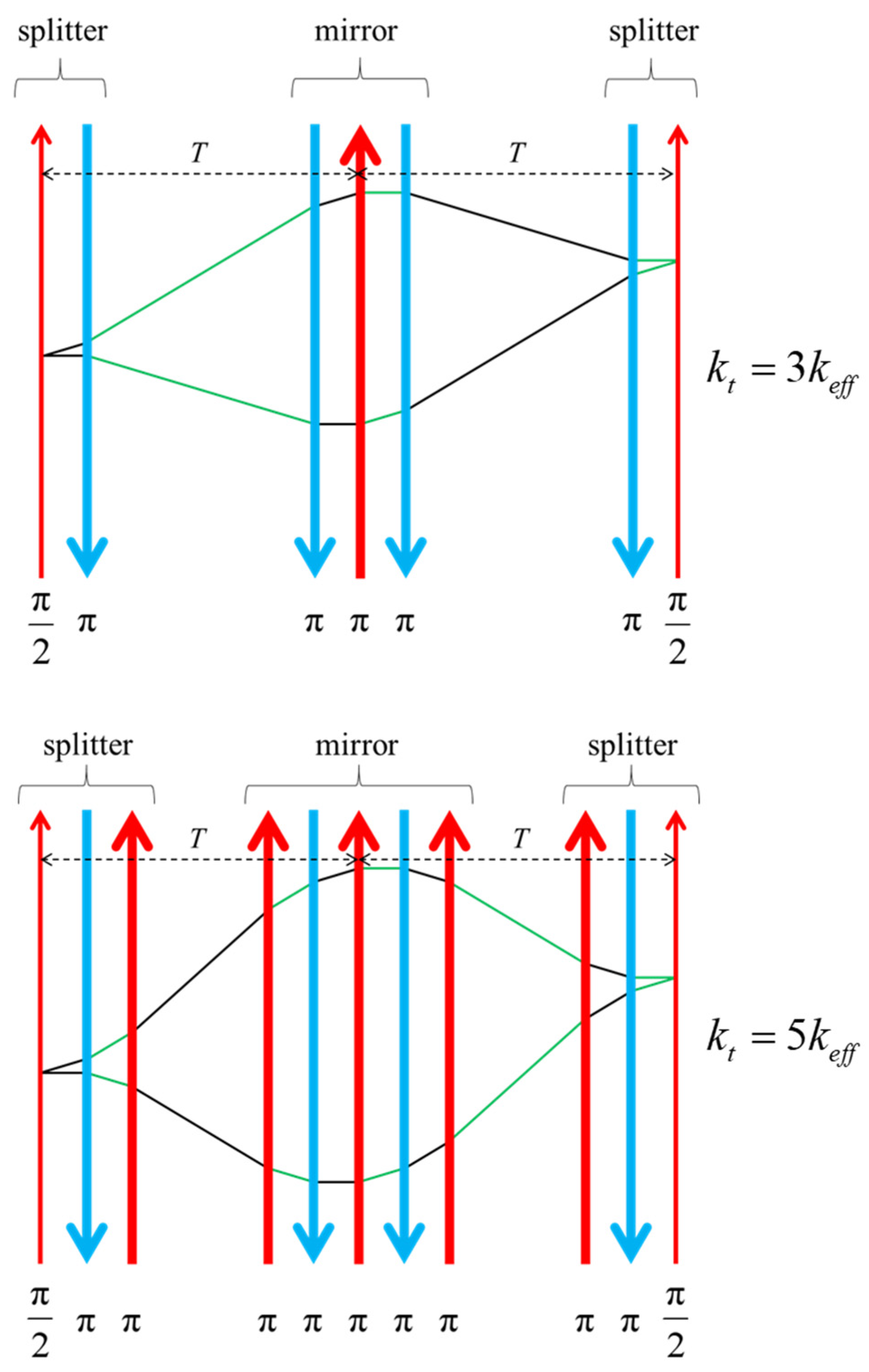
Techniques such as Bragg diffraction and Bloch oscillation in optical lattices require atoms with sub-recoil velocity spreads in the longitudinal direction, requiring either velocity selection or increased cooling, which adversely affect the signal to noise ratio as well as the repetition rate. As such, we focus here on the method of using additional Raman pulses [
15,
16,
17]. The protocol for realizing LMT using this method is illustrated in
Figure 7. Additional Raman pulses in alternating directions are added to the conventional
pulse sequence.
The modeling of the motion of the center of mass of each atom was discussed earlier in
Section 3. Here, we describe the evolution of the internal states of each atom under this Raman pulse sequence. The internal state is modeled as a three-level system: the ground state
, the excited state
, and the intermediate state
. The pulses induce Raman transitions among these three states. The frequency and the wavenumber of the first (second) Raman beam are denoted as
(
) and
(
). Due to conservation of linear momentum, a pair of Raman beams couples the three states
,
, and
. The resulting Hamiltonian, in the basis spanned by these three states, can be expressed as follows:
where
and
. Here,
is defined as
and
as
. With the adiabatic elimination [
35], we obtain the effective two-level system Hamiltonian, in the basis spanned by states
and
:
If we set
,
, and shift all energy levels by an amount that makes the energy of state
vanish, we have:
where
. From this Hamiltonian we see a detuning caused by the Doppler shift given by
, as well as the effective Rabi frequency given by
. In addition, the adiabatic elimination also gives us the effective decay rate [
28] between the states
and
:
The total decay rate for the coherence between states
and
is then given by:
The D
2 line decay rate from 5
2P3/2 to 5
2S1/2, expressed as
, is about 2π × (6 MHz) for
87Rb. Only the atoms that have not experienced spontaneous emission keep their phase information. The fraction of atoms that have decohered by the end of the interferometry process is given by
, where
is the total duration of all the Raman pulses. With this model, we can simulate the signal for a PSI–LMT, while taking into account the complexities caused by detuning. The effect of spontaneous emission is considered later in a heuristic manner. In the model discussed in
Section 3, we assumed all
components to be resonant, which is approximately valid if the effective Rabi frequency is much larger than the Doppler shift. In order to account for more general conditions, in our simulation we used different Hamiltonian operators for different
components, corresponding to Equation (16).
The computation process for determining the PSI signal can be summarized as follows. As we illustrated before, each pure state in Equation (10) evolves independently. Therefore, we can calculate the evolution of each pure state and add them up according to the initial weight in the end. In each pure state, consider a single point in the k-space as an example of the simulation. The state will see the first π/2 pulse dictated by the Hamiltonian in Equation (16), and become a superposition of a point (in the k-space) of the ground state and a point (in the k-space) of the excited state. Then they evolve freely for time T. The free evolution is dictated by the Hamiltonian in Equation (16) with . Then they see the π pulse also dictated by Equation (16). The beams of the π-pulse are rotated by the angle (where is the rate of rotation). The π-pulse is imperfect due to the Doppler shift detuning, resulting in a state that is a superposition of two points (in the k-space) of the ground state and two points (in the k-space) of the excited state. After another free evolution of T, they see the final π/2-pulse and become a superposition of four points (in the k-space) of the ground states and four points (in the k-space) of the excited states. With the final state in the k-space, we can calculate the state in the position space.
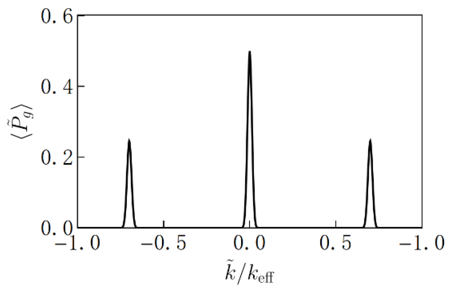
Using this approach, we simulated the signals for the case of atoms released from a harmonic oscillator trap, as shown in Equation (10), for
, with the following parameters:
,
,
, and
. Here, we chose an unrealistically small size of the trap, in order to elucidate the behavior of a system that is very close to an ideal point source. The simulation results for this case are shown in
Figure 8. The main difference from the result shown in
Figure 2 is that the height of the signal peak is shorter since the detuning resulting from
(the difference in the momentum in the z-direction between the two arms, as defined earlier in
Section 2) was taken into account. There is also a little difference in the width of the signal peak. For the LMT case shown in panel B, there are also some small peaks in addition to the main signal peak. This is because the pulses are not ideal. For example, a pulse that is nominally designated to be a π-pulse does not fully transform a ground state to an excited state, or vice versa, but will leave some residual. The small peaks are the consequence of the interference involving the residuals.
As can be seen from comparisons between the PSI and LMT–PSI results shown in
Figure 8, the LMT process produces a larger separation for the signal peaks in the Fourier transform domain, thus making it more sensitive for measuring rotation. At the same time, the amplitudes of the signal peaks are smaller, which in turn would represent a reduction in the effective signal to noise ratio, and a corresponding reduction in sensitivity. The actual improvement in sensitivity would be determined by both factors. In this context, we consider first the fact that the degradation of the signal (both in terms of the reduction in the amplitudes, and the appearance of additional peaks) can be countered by increasing the effective Rabi frequency:
. As we mentioned before, the maximum heights for the signal peaks occur when
.
Figure 9 shows the comparison between signals for different effective Rabi frequencies, with
. Panel A in
Figure 9 corresponds to the case where
and
. Panel B (which is the same as Panel A of
Figure 8) corresponds to the case where
and
. As can be seen, the amplitudes of the signal peaks increase for the larger value of the effective Rabi frequency, and the additional peaks almost disappear completely.
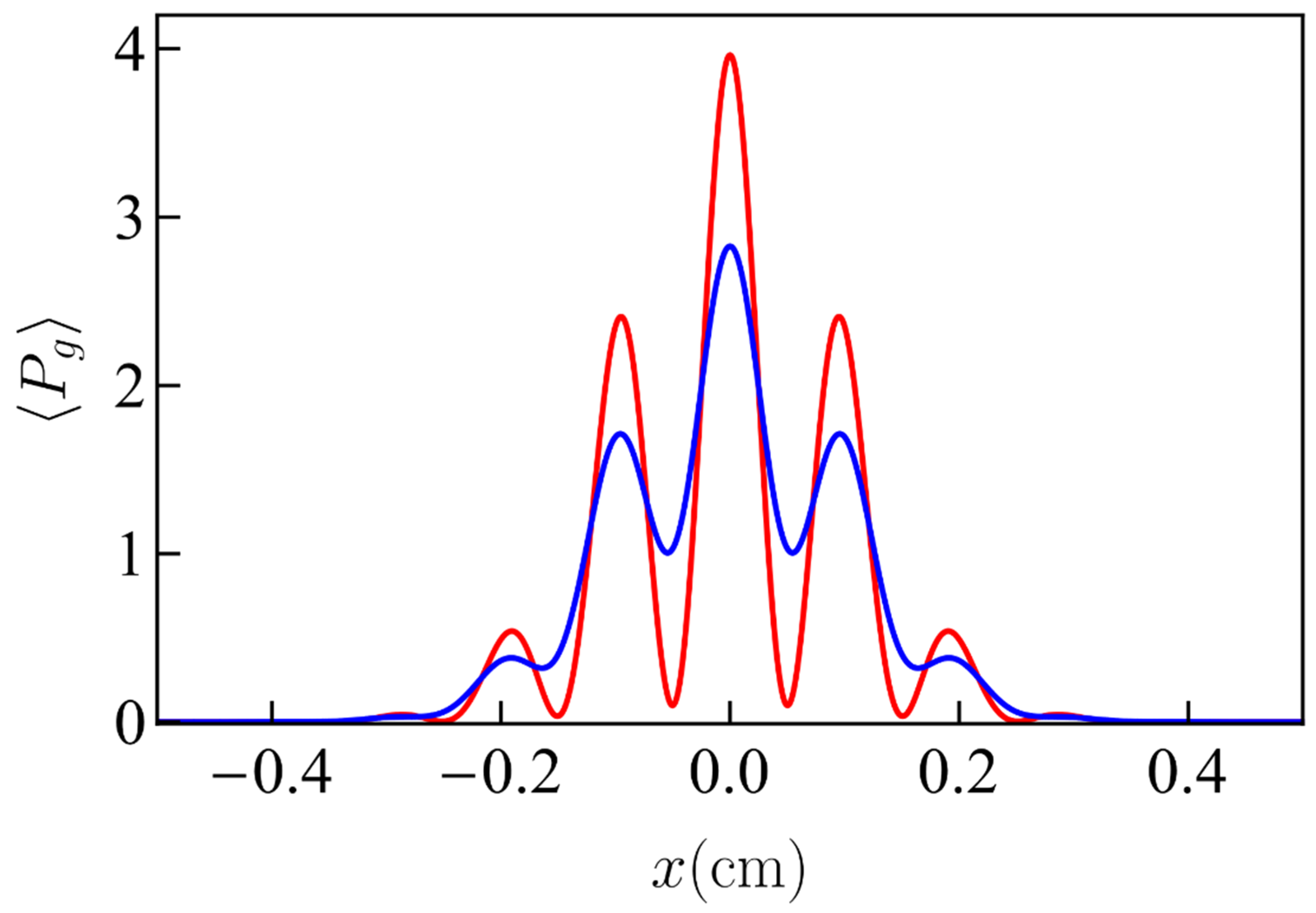
Figure 10 shows a signal for
with
and
. We can see in this case that the signal is still very close to the ideal signal that does not take into account the effect of detuning. Simulations with larger
require extremely large amounts of computational resources because we used a fully quantum model. Attempts will be made in the near future to extend the simulation to much larger values of
. In what follows, we present a systematic analysis for estimating quantitatively the expected net enhancement in sensitivity as a function of the effective Rabi frequency and the value of
, while taking into account the effect of spontaneous emission heuristically.
Before proceeding with this analysis, we note for clarity that the results presented in
Figure 8,
Figure 9 and
Figure 10 have been computed with the augmented quantum model. However, if the semi-classical model were used instead, the results would be very similar, even when the Doppler detuning is taken into account, with the difference being very small of the order of what is shown in
Figure 6d. Furthermore, as noted above, carrying out the analysis with the augmented quantum model for a significant value of N requires enormous computational resources. Given that the difference between the results produced by the semi-classical analysis and the augmented quantum model is very small, undertaking such an analysis was not deemed critically important at this point. Instead, in order to estimate the degree of enhancement achievable using LMT for increasing values of N, in what follows we make a simplifying assumption that eliminates the distinction between the augmented quantum model and the semi-classical model. Specifically, in the estimation of the contrast of the fringes (equivalently, the height of the signal peak in the Fourier transform domain) we ignore the momentum distribution of the atoms and assume that all atoms see the same detuning. Therefore, the effect of the Doppler shift detuning will produce only an overall reduction in the signal peak. Consequently, the quantized model for the motion of the center of mass of the atoms becomes irrelevant. The spontaneous emission also only results in an overall reduction in the signal peak, and thus does not depend on the quantized model for the motion of the center of mass of the atoms. As such, the rest of the results that follow in this section are based on the semi-classical model.
The value of
, the height of the signal peaks in the Fourier transform domain, defined earlier in
Section 2, is determined primarily by the transition efficiency of each
pulse and the effective spontaneous emission. To simplify the analysis, as noted above, we ignore the dependence of the effective Rabi frequency on the momentum of the atoms. Therefore, we define the constant effective Rabi frequency as
. We define the propagator of the quantum state of the atom due to a Raman pulse,
, by the expression
. This propagator including the effect of detuning caused by the Doppler shift can be expressed as:
where
and
is the detuning caused by the Doppler shift. In principle, even the atoms following the same trajectories will have a thermal distribution of momenta. However, in the LMT case with
N much larger than unity, the thermal momentum is very small compared to
. With
, the typical thermal momentum,
, is only ~
. Therefore, we ignore the thermal momentum distribution of the atoms, which means that atoms following the same trajectories experience the same detuning. Generally, it is difficult to handle this propagator analytically. However, in the limit that
, we can make approximations to Equation (19) and make it more manageable. The transition efficiency of a π-pulse derived from Equation (19) is:
where
,
is the Doppler shift inducing detuning for an atom with momentum
, and
. In the last step of Equation (20), we assumed that we could make
different for each Raman pulse, such that for all pulses
. When
, the value of
is only ~0.1. Therefore, it is reasonable to consider
a small quantity. Only considering the effect of the imperfection of the π-pulses, the height of the signal peak for
is reduced by a factor of the multiplication of the transition efficiency of all the π-pulses times the spontaneous decay term, that is:
Then the logarithm of the height is:
Keeping only the leading term of
, we have:
The last step in Equation (23) is valid because normally, as long as we have a reasonably large
, the value of
is very small compared to 1. For example, if
and
, we have
. Therefore,
. With a reasonably large
, we also note that
. Here, we do not consider the effect of the finite initial size of the atomic cloud, so that
. In this expression,
can be considered the ideal height ¼, and thus
. Substituting the expressions of
and
into the expression of the improvement factor, we can calculate the natural logarithm of the improvement factor:
The optimal value of
for maximizing
is:
The natural logarithm of the improvement factor for this
is:
We see that the maximum value of
ε is given by:
This value of
ε occurs for an optimal value of
, given by:
We can see from Equations (27) and (28) that both
and
are proportional to
.
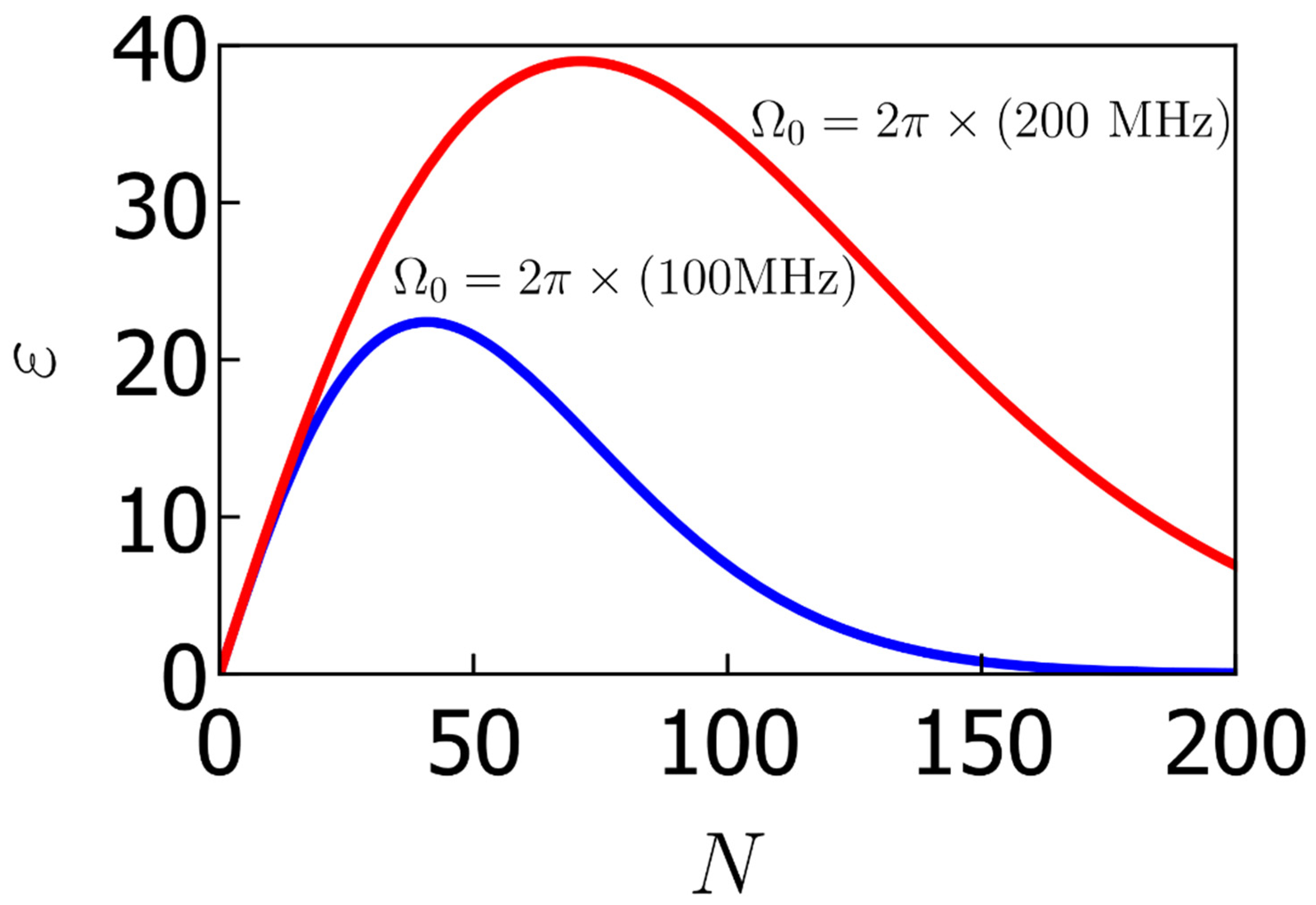
Figure 11 shows how
varies with
for
(red) and
(blue) when only the effect of the imperfection of the π-pulses is considered. We see that
for
with
. With this Rabi frequency, when
, the optimal
is 2π × (1.7 GHz), according to Equation (25). It is also shown in
Figure 11 that
can significantly affect the maximum improvement LMT can achieve.
In the analysis above, we only considered the effect of imperfect π-pulses on the signal. Next, we incorporate the effect of the finite initial size discussed in
Section 2 into the calculation of the signal. Adding the contribution of the finite initial size to the reduction in the height of the signal peak shown in Equation (4), Equation (23) is modified to be:
and Equation (24) is modified to be:
Here,
is the initial (final) size of the atomic cloud, as defined earlier in
Section 2. The optimal detuning will not be affected by the initial size of the atomic cloud because the term contributed by the finite initial size does not depend on the detuning
. Therefore, with the optimal detuning, we have:
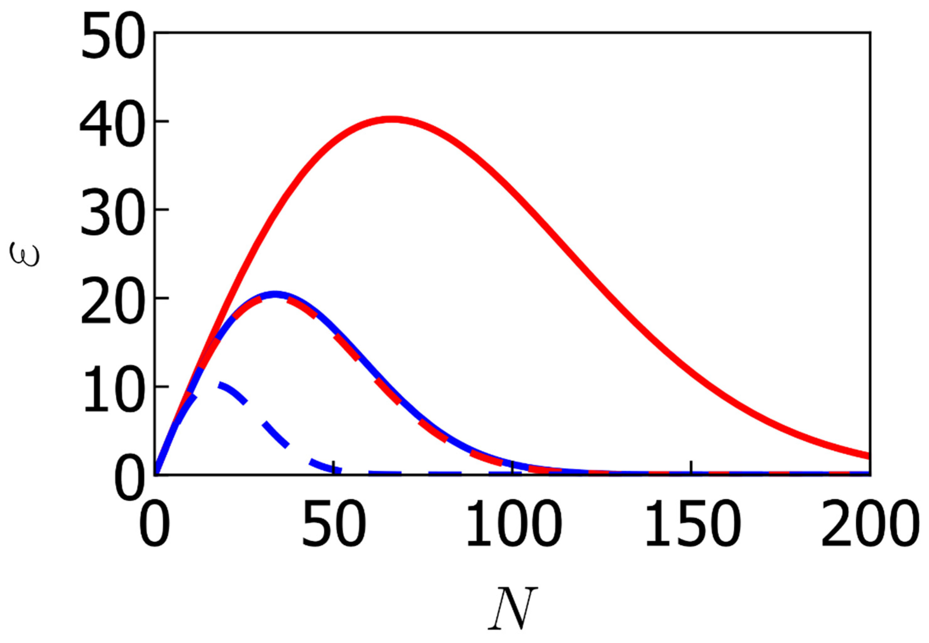
Figure 12 shows the relationship between
and
given by Equation (31), with
,
,
. The black dotted curve shows the case where
, which is identical to the red curve in
Figure 12. The red curves are the plots for
, while the blue curves are for
. The solid (dashed) curves correspond to an angular velocity of 1 (2) μHz. We can see that if
, the correction to the signal due to the finite initial size is very small. In this case the conclusion derived above that
for
is still valid. We can also see that the correction to the signal due to the finite initial size decreases as the angular velocity we want to measure decreases. Therefore, LMT is more advantageous for measuring smaller rotations.
To recap, both
Figure 11 and
Figure 12 are plots of the improvement factor
ε versus
.
Figure 11 shows the cases where we only considered the effect of Doppler shift detuning and spontaneous decay.
Figure 12 shows the cases where we additionally took into account the effect of the finite initial size of the atomic cloud. In
Figure 11, the blue curve shows the case where the one-photon Rabi frequency was 100 MHz and the red curve was 200 MHz. We can see that a higher one-photon Rabi frequency will enable us to improve the PSI more with LMT. We used a one-photon Rabi frequency of 200 MHz for all curves in
Figure 12. In this figure, the red curves (both solid and dashed) are plots for the initial size of the atomic cloud
, and the blue curves for
. The solid curves (both red and blue) are for the angular velocity of 1 µHz, and the dashed curves are for 2 µHz. We can see that both a smaller initial size and a smaller angular velocity will enable us to improve the PSI more with LMT. With
,
, and an angular velocity of 1 µHz, the effect of the finite initial size of the atomic cloud is not obvious and thus the result becomes very similar to the red curve in
Figure 11 (reproduced as the black dotted curve in
Figure 12).
It can be seen from the discussion above that the value of
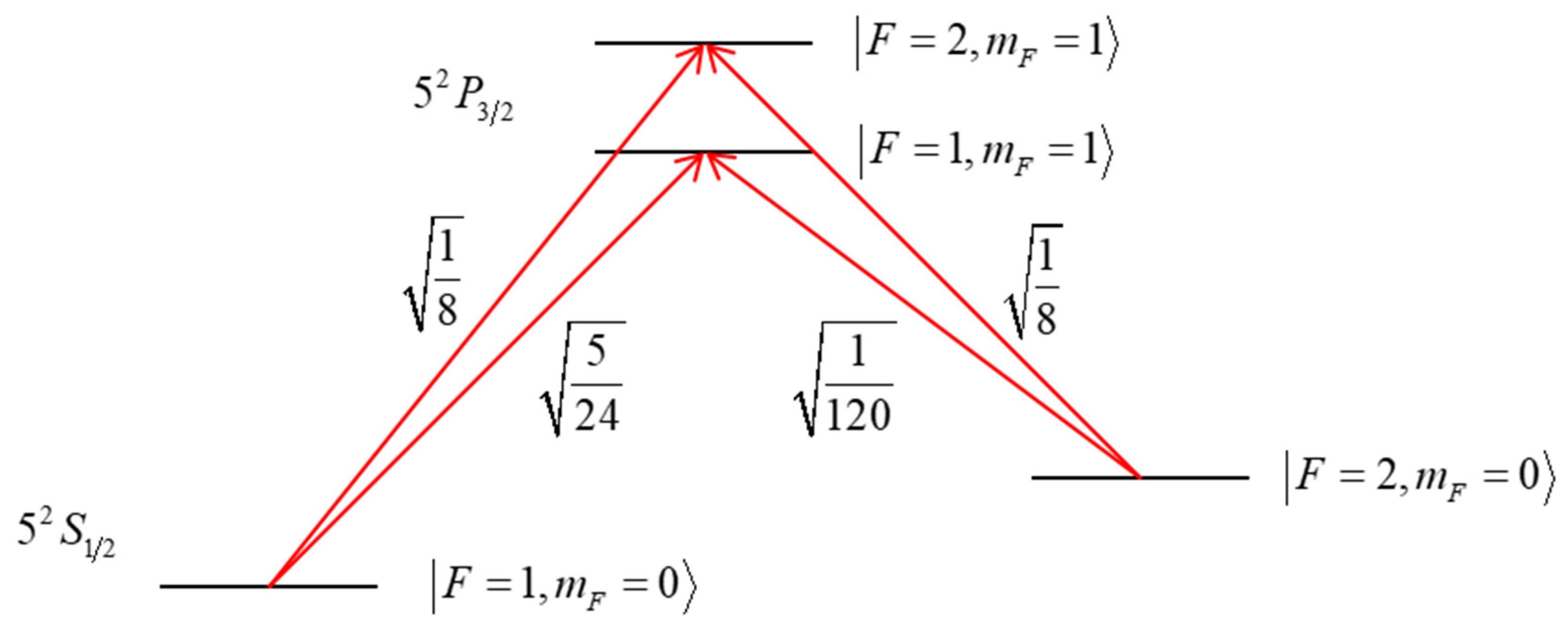
is very important for the performance of the LMT-PSI. Therefore, we discuss here the relationship between the experimental parameters and
. For
, we assumed the ground state
to be
, and the excited state
to be
. In most implementations of Raman-pulse-based atom interferometers, the beams are circularly (σ) polarized [
36]. If the beams are
polarized, the intermediate state
consists of two states:
and
of the
manifold. The corresponding transition matrix elements [
37] are shown in
Figure 13. For the cycling transition from
to
, an intensity of 3.34 mW/cm
2 yields
. For a given intensity on each leg of the Raman transition, we can use this information to determine the effective Rabi frequency for each of the two Raman transitions, treated separately, and the net effective Rabi frequency would be the sum of these two effective Rabi frequencies. If we assume that each leg has the same laser intensity and consider the fact that the energy separation between the two upper levels (~157 MHz) is negligible compared to the detuning, then it is easy to see that the effective Rabi frequency for the lower Raman transition is weaker than that for the upper Raman transition by a factor of
. If we consider the upper Raman transition only, the intensity needed for the condition of
is ~3.7 W/cm
2. When both Raman transitions are taken into account, an intensity lower by a factor of 3/4 (i.e., ~2.8 W/cm
2) would produce the effective Rabi frequency corresponding to
in our model presented above [
38]. Such an intensity can be achieved, for example, by using a tapered amplifier on each leg of the Raman transition.
There is another technique that can potentially decrease the effect of the detuning. At the beginning, when the momentum difference between the two arms is small, both arms are addressed with the same Raman beams. When the momentum difference between the two arms become large enough, we can address them with different Raman beams so that both arms are resonant to its own Raman beams and far detuned from the Raman beams for the other arm. This technique works well for very cold atoms. However, for an atom at a temperature of 6 μK, the thermal momentum is about . It is not obvious whether this thermal momentum is sufficiently small in comparison to the total momentum transfer for this technique to improve the performance of the PSI–LMT significantly. This issue will be investigated in the future.


 ,
, 


