Model-Free Current Loop Autotuning for Synchronous Reluctance Motor Drives


Department of Management and Engineering, University of Padova, Stradella San Nicola, 3, 36100 Vicenza, Italy
*
Author to whom correspondence should be addressed.
Automation 2020, 1(1), 33-47; https://0-doi-org.brum.beds.ac.uk/10.3390/automation1010003
Submission received: 1 September 2020
/
Revised: 15 September 2020
/
Accepted: 20 September 2020
/
Published: 24 September 2020
Abstract
:Synchronous reluctance motors are arousing lively interest as a possible alternative to the less efficient induction motors. An open issue is the effective tuning of the inner current loops because of the nonlinearity that cannot be overlooked. The present paper uses a relay feedback approach to perform autotuning without resorting to any parameter knowledge. The tuning is iterated at different working points, to get a uniform current control bandwidth everywhere. Unlike many solutions in the field, the algorithm is truly autonomous, in the sense that it also suggests a correct value for the bandwidth specification. The paper includes both simulation and experimental results, obtained on a laboratory prototype.
1. Introduction
In the mainstream of energy and environmental global paradigms, the electric drives technology is moving toward more efficient motors and more intelligent control systems, able to minimize the human intervention at any stage of the product life, while ensuring the best possible performance.
Synchronous reluctance (SynR) motors conjugate the efficiency of synchronous machines with the low-cost structure and absence of the permanent magnet (PM) typical of induction motors. In the light of the above frame, they represent a promising alternative in many low cost, mid-performance applications.
Performance achievement is directly linked to the correct tuning of the inner current control loop, which is fully responsible for torque dynamics. The opportunity to spare commissioning time suggests an automatic tuning that unfortunately is complicated by the nonlinearity of the magnetic model [1].
In literature, the problem has been faced in different ways. In [2], an online tuning adaptive controller is proposed, based on the least mean-square algorithm. A nonlinear programming optimization technique is used to improve the convergence rate, giving the system enhanced transient responses and tracking capability. Anyway, the complexity of the algorithm and the high number of parameters to be tuned somewhat clashes with the demand for cost-effectiveness and simplicity that characterise SynR motor drives.
A different approach, also characterised by marked complexity, is reported in [3]. The paper proposes an enhanced brain emotional learning-based intelligent controller for a synchronous reluctance motor (SynRM) drives. The standard proportional-integral (PI) controllers are replaced by emotional learning and decision-making mechanisms-cues certainly fascinating—but assessed as rather over-the-top for the goal at hand.
As a more realistic alternative, an accurate magnetic model can be used in combination with conventional PI controllers, as in [4]. The PI gain scheduling and synchronous axes decoupling are based on a comprehensive model. Thus, the complexity is shifted from current loop tuning to offline motor characterisation. This may help, but the whole system still relies on a delicate and very involved neural networks algorithm.
Reference [5] discusses nonlinear proportional-integral (PI) current control assuming that the flux linkage maps are obtained by either Finite Element analysis (FEA) or measurements.
A simple autotuning controller that allows the field engineer define the closed loop dynamics by specification of the current peak response time and overshoot is proposed in [6]. Again, it hinges the motor model, which is obtained by a recursive least squares algorithm.
In the end, analysis of the literature indicates that the weak point of the SynR motor drives is inherent uncertainty in the model. This seems to push towards a calibration of the current loop as free as possible from the motor parameters. On the other hand, the simplicity of proportional-integral controllers is still attractive.
This work gives an answer to both issues. The conventional PI controllers are tuned automatically by an algorithm that does not hinge on the knowledge of any motor model. A well known method, i.e., the relay autotuning method firstly proposed in [7], can be fruitfully adopted toward this aim. In a nutshell, the method consists of the automation of the Ziegler–Nichols sustained oscillation method through the use of an online relay experiment. The relay autotuning method does not require a model of the process to be controlled. The principle of operation is known and already applied to industrial PLC ([8]) and PMSM motor drives ([9]). However, the latter work deals with an isotropic synchronous motor where the magnetic model is linear.
In this paper, the relay autotuning method is brought to the specific world of highly nonlinear SynR motors. In contrast to past research efforts, the algorithm has to be tailored for the motor under test knowing this important characteristic. The task is less trivial than expected. The marked nonlinearity and the high values of phase inductance call for special attention in implementation. As a distinctive feature, the result is a true autonomous tuning algorithm, in the sense that it alone suggests the most likely value for the bandwidth, relieving the human operator from this task. The proposed algorithm does not require a model of the motor, in accordance with the model-free characteristic of relay autotuning methods [7], but it has been developed based on the fact that the model is nonlinear, and not on the exact knowledge of such nonlinearity characteristic. Furthermore, an automatic procedure aiming at obtaining the best current control bandwidth is also proposed. Finally, the tests are carried out at standstill, thus no rotor movement is either necessary or produced by the proposed algorithm.
The paper is organized as follows. Section 2 gives a short recollection of the models of both the SynR motor and the inverter. The key concepts for the implementation of the current control loop of an inverter-fed SynR motor are also discussed.
Section 3 presents the basics of the relay feedback autotuning theory. It includes suitable mathematical background and some insights for real implementation of the proposed autotuning procedure.
2. AC Drive System Overview
In order to design the most suitable autotuning algorithm for the process under consideration, it is useful to describe the general model of a SynR motor fed by a three phase inverter. The peculiarities and characteristics of both motor and inverter transfer functions are described in Section 2.1 and Section 2.2.
2.1. Synchronous Reluctance Motor Model
The control of the SynR motor currents is performed in the reference frame synchronous with the electrical position of the rotor . The alignment of the d-axis is chosen along the position that features the minimum magnetic reluctance with respect to the stator windings. The motor voltages balance equations are written using matrix notation as:
where , and are the stator voltages, currents, and magnetic flux linkages, respectively, R is the stator windings resistance, is the electric speed, p is the number of pole pairs, and is the mechanical speed. The matrix is defined as a static rotation of , i.e., .
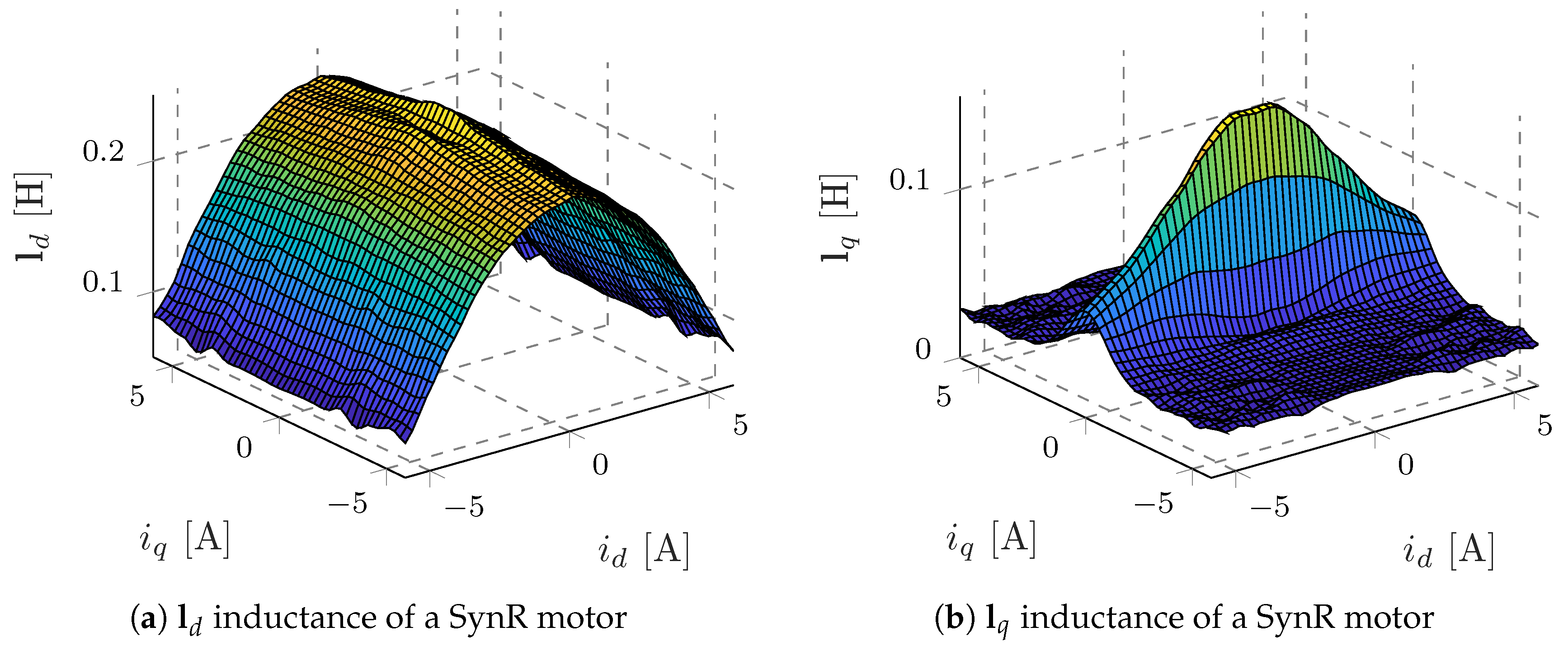
The SynR motor is strongly affected by magnetic saturation even inside the nominal load range, as depicted in Figure 1. The curves represent the differential inductance maps of the motor used in the experimental tests. The complete maps were obtained by means of dedicated tests, such as the method proposed in [10]. It is worth noting that a dedicated test rig is required in [10], which is not possible in many industrial applications. Due to the saturation, the magnetic paths suffer cross-coupling, so that the flux linkages in (1) are functions of both currents .
However, knowledge of the nonlinear relationships between flux linkages and currents is crucial for the model-based current controller design methods.
In order to simplify the design of the current controllers, which are often proportional-integral controllers (PI), the magnetic flux linkages are written as function of currents only. The motor model (1) is rewritten as:
where and are the differential and apparent inductances. In the sequel, the dependence of both inductances on currents is understood.
Despite the additional complexity introduced by the two nonlinear maps, two considerations allow to facilitate analysis of the mathematical motor model (2). On one hand, the speed dependent term can be discarded by considering the rotor at standstill. This is a common assumption for autotuning techniques. On the other hand, the axes cross-saturation effects can be ignored by assuming a diagonal inductance matrix . This is true when only one current is not zero, whereas the other one is maintained at zero value. Under the previous two hypotheses, the motor voltages balance can be rewritten as
and the torque T equation becomes
It is important to highlight that, when the current of one axis is null, the magnetic flux of the same axis is null as well. Therefore, the torque produced by the SynR motor is not zero only if both currents are nonzero.
The currents fully handle the torque production and the proposed model shows that they can be independently regulated by two PI-like controllers.
In case of constant inductances, two conventional PI controllers should be able to guarantee the desired bandwidth within the whole operating region of the motor. Since for a SynR motor this is not the case, it is impossible to guarantee stable current dynamics throughout the working region. This calls for more intricate solutions. In this paper, the PI structure is preserved, while variable gains are considered and sought by the autotuning procedure.
2.2. Voltage Source Inverter Model
The SynR motor is supplied by a voltage source inverter, operating according to the field oriented control (FOC) principle. The inverter suffers from several non-idealities due to the real behaviors of the switches. Nonetheless, many viable solutions to compensate for these side effects have been proposed in the literature (see, e.g., [11,12,13]). In the following, a well-compensated voltage inverter is assumed, so that the model reduces to a static delay, linked to the digital synthesis of the reference voltages. Therefore, the inverter transfer function is
which is usually approximated as
with , with being the switching period.
3. Relay Feedback Autotuning Basics
As discussed in Section 2.1 and Section 2.2, the inverter-motor set can be represented as a first order plus time delay (FOPDT) model. A relay feedback autotuning technique was implemented in [9] for an isotropic synchronous permanent magnet motor, based on the original work presented in [7].
In principle, the same technique could be applied to a SynR motor, although the nonlinear behavior of the magnetic flux linkages relationships with the current reported in Section 2.1 poses an important limitation. In fact, the autotuning method proposed in [9] is valid for one working point, i.e., only at .
This paper aims at preserving the manifold benefits of the relay feedback approach, trying to extend its application to an SynR motor AC drive. The autotuning procedure for a single working point is first described in Section 3.1. Several hints and comments on how to achieve the maximum reachable bandwidth are reported in Section 3.2. Finally, the complete procedure is described in Section 3.3.
3.1. Single Value Autotuning
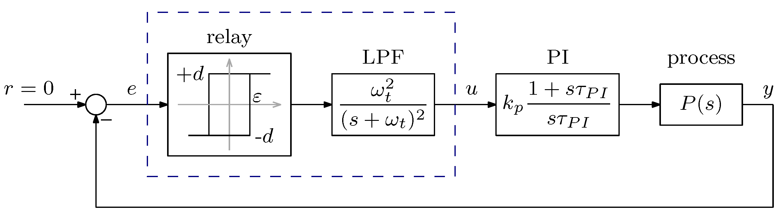
The main blocks of the autotuning procedure are sketched in Figure 2. The unknown process is assumed to be a FOPTD model, and it is preceded by PI block expressed in Bode form. During the tuning procedure, relay and low-pass filter (LPF) blocks are introduced in the direct control chain, but they will be removed at the end of the tuning procedure. The relay block presents a hysteresis and output amplitude d. The LPF is of second order and its cut-off frequency is equal to . It is interesting to note that the additional blocks, highlighted by the dashed closed line in Figure 2, of the proposed autotuning method can be implemented inside the control scheme. Therefore, no additional hardware is required.
The output of the relay is a square wave signal, and it produces a permanent perturbation on the system, i.e., the stimuli necessary for the proposed relay-feedback autotuning method. The speed of the generated oscillation is denoted , and the identification of the direct chain reveals its position in the Nyquist diagram.
At each instant, the equation is imposed by the system autotuning architecture. In particular, considering the Laplace transforms of these variables and observing their phases, it holds that:
which means that the direct chain phase is equal to and so the point is the crossing of the function with the negative real axis of the complex plane. Observing this result, it is already possible to focus the target of the tuning procedure. In order to obtain a properly designed PI controller, it is enough to note that, for a given desired bandwidth and phase margin , Equation (7) evaluated at should yield in .
The relay is a nonlinear component whose behavior can be modeled according to the Fourier Series. As shown in [9], it is independent of and dependent on parameters and a, which is the amplitude of the oscillation of y. If , the phase lag becomes negligible, improving the model robustness. The hysteresis of the relay is introduced to enhance the robustness to noise measurements and avoid spurious commutations of the relay. After an initial measurement of the noise which affects the control system, the threshold can be chosen. In particular, the amplitude a of the oscillation can be selected as a multiple of in order to guarantee precise oscillation measurement (in this paper ).
The low-pass filter introduces a phase lag equal to
The value is tuned to guarantee that when the system in Figure 2 is oscillating at the desired closed loop bandwidth ().
The phase lag introduced by the PI controller depends only on , and it spans from to 0. The process to be controlled exhibits low-pass filter behavior and it introduces an additive phase lag which is unknown and dependent.
From the analysis of the blocks, it can be inferred that, during the tuning, for constant and invariant processes, depends only on . In particular, if is increased, the negative phase lag due to the PI subsystem is reduced and must therefore be compensated, according to (7), increasing the negative lag introduced by the other blocks, i.e., increasing . On the contrary, if is decreased, also decreases. This relationship permits specification of a method for the tuning of . Focusing on varying , is changed until it is equal to the desired bandwidth. In this condition, the additional blocks introduce a phase lag equal to the phase margin. The phase lag of the series between the control block and the process (which will be a direct chain once the other two elements are removed) is exactly equal to .
When the oscillation frequency reaches the desired closed-loop bandwidth, the zero of the PI block is tuned. The target is now determination of the gain which permits achieving zero attenuation at the desired cross-over frequency. The input u to the PI block and the output y of the process are measured. The amplitude ratio of the two variables represents the attenuation introduced by the series connection of the controller and the process at the desired control bandwidth and it has to be made equal to one. The requested can be evaluated accordingly.
3.2. Maximum Achievable Bandwidth
It can often happen that, given a certain process dynamics, the desired bandwidth is not achievable. Moreover, the typical industrial specifications do not precisely define the closed loop bandwidth of the system but request a minimum value which characterizes the poorest performance of the system that is acceptable. An autotuning procedure that is able to automatically detect if a target bandwidth is not possible or extract the maximum achievable bandwidth (MAB) from a given process could be very useful.
Considering the autotuning system of Figure 2, if the target bandwidth is increased, the negative phase lag of all the blocks evaluated at increases, except for that of the PI block. Therefore, in order to guarantee the required phase margin, the zero of the PI block must introduce more positive phase increasing . This concept can be applied until the zero of the PI block corresponds to a frequency of such low magnitude that its modification does not produce any other positive effects (namely lower than three decades with respect to the requested bandwidth). For these values of , the measured during tuning do not increase further. Thus, the MAB can be estimated observing how progresses with respect to the desired bandwidth for a PI block tuned with a zero placed below three decades with respect to this latter. If the measured is lower than , it means that the system (with the LPF included) already introduces a phase lag equal to at a frequency which is lower than the requested . The phase margin at will surely be less than the target value. In this case, a different control strategy or softer dynamic specifications (reducing the required bandwidth or phase margin) should be chosen.
3.3. Proposed Adaptive Pi Autotuning Procedure
The autotuning procedure described in Section 3.1 can be adapted to work at different working points of the motor by imposing a DC current offset (). This solution permits exploration of the possible magnetic saturation effects on the current control performances of a SynR motor drive. In fact, the motor inductances may vary with the working point, and a correction of the controller gains should be performed to guarantee the stability at each working condition. Hence, as suggested in [4], an adaptive PI approach can be chosen. The gains of the controller can be obtained by executing iteratively, for different levels of current, the relay-feedback autotuning procedure proposed in Section 3.1.
Particular attention should be paid to the amplitude of the perturbation. As a matter of fact, it must be chosen as a trade-off between having negligible effects of the relay () and the necessity to maintain linear motor behavior during the procedure in particular for the evaluation of .
The ability of the self-commissioning procedure to operate at a standstill is very valuable. In this paper, the standstill operations are obtained for a SynR motor drive by performing the autotuning only imposing one current at a time. As mentioned in Section 2.1, the torque production is null if one current is at zero value. Thus, by performing the autotuning procedure one axis at a time, while keeping the other axis current at zero, the standstill operations are guaranteed.
Because of the strict relationship between the evolution of the oscillation frequency with respect to and the MAB, it is possible not only to autotune the current controllers but also to maximize their performance. These are limited by the motor electrical dynamics that changes during the autotuning. In particular, the worst condition for the tuning of the d axis controller is . In this working point, the inductance value reaches the maximum. The minimum value of the MAB along the motor working range corresponds to this condition.
In order to find a sub-optimal solution, an iterative procedure is proposed by starting from maximum control specification, i.e., very high control bandwidth and phase margin. The maximum control bandwidth value is gradually decreased until its value and the desired phases margin are reachable. The initial bandwidth can be chosen as equal to half the switching frequency, which is the theoretical maximum value of the discrete control system bandwidth by the Shannon frequency. The phase margin is chosen in accordance with the desired degree of stability. The value of is chosen in order to maximize the benefits of the PI in the phase lag of the open loop system (namely three decades below the required bandwidth). The identification of the system is started by enabling the relay operations and measuring the oscillation period. The procedure, even with large , will measure an oscillation with frequency less than the desired bandwidth. Therefore, by gradually decreasing the required bandwidth, the maximum value in the worst condition (axis d, ) can be detected. The bandwidth value founded by the proposed procedure is thus adopted and it is iteratively performed tabulating the obtained PI gains for the next use during the motor control.
To summarize, the adaptive autotuning procedure consists of the two Algorithms 1 and 2. The former is performed firstly with the aim of determining the MAB . The latter is iteratively run for both axes and different current offsets r obtaining the adaptive PI gain maps which guarantee the same performances at each working condition of the motor. The function systemPerturbation stands for enabling the relay of the considered axis, increasing its output values since the current oscillation reaches the desired amplitude a and measures the frequency of the generated oscillation.
| Algorithm 1: Search of the MAB |
 |
| Algorithm 2: Single value autotuning |
 |
4. Simulation Results
The proposed autotuning algorithm was first tested on a virtual simulation environment. The aims of the simulations include the verification of the effectiveness of the technique and its functioning. Model features were tailored to the real test bench used for the subsequent experiments, whose nameplate data are reported in Table 1.
The autotuning parameters are listed in Table 2.
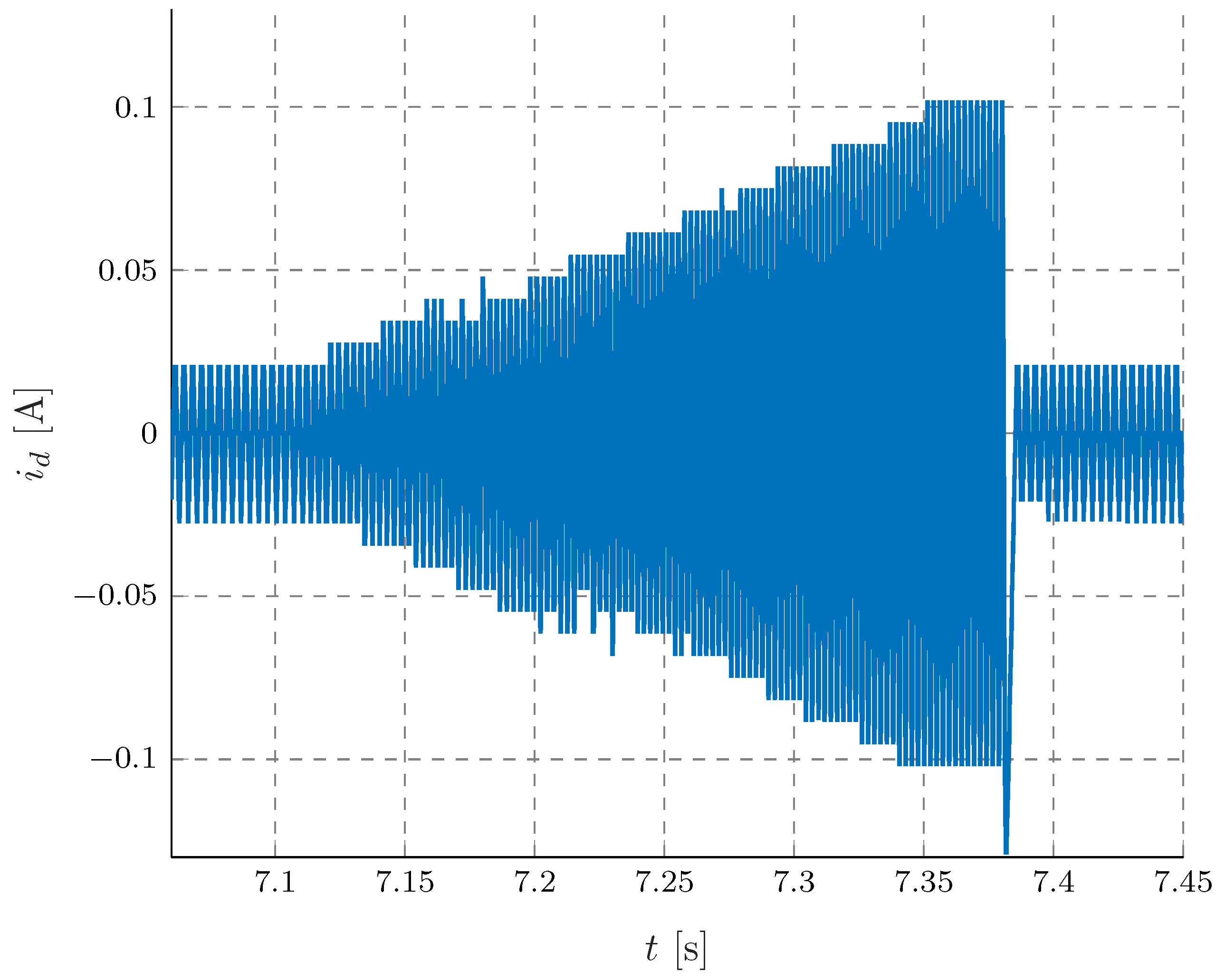
The autotuning procedure begins with the search along the MAB along the d axis current with a current offset equal to zero according to Algorithm 1. With an initial target bandwidth surely higher than the maximum achievable one (for example, , ), a first perturbation of the system is performed, activating the relay and LPF digital blocks. When subjected to a perturbation, the measured current evolves sinusoidally as in Figure 3. The output of the relay is gradually increased until the amplitude of the current oscillation is in absolute value both for the positive and the negative peaks. Then, the oscillation is maintained for 20 periods in order to measure the oscillation frequency.
The measurement, the output of the relay, and the output of the filter during the measurement are shown in more detail, for clarity, in Figure 4.
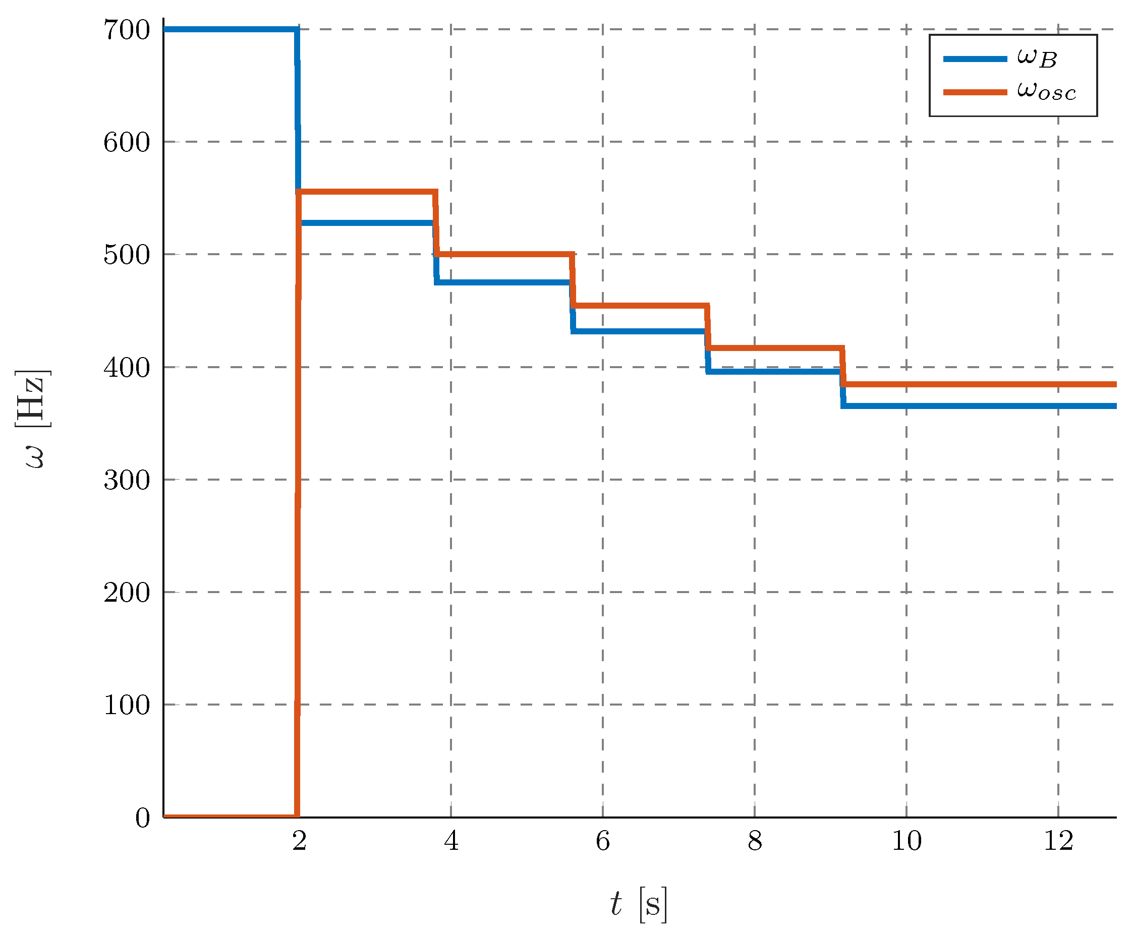
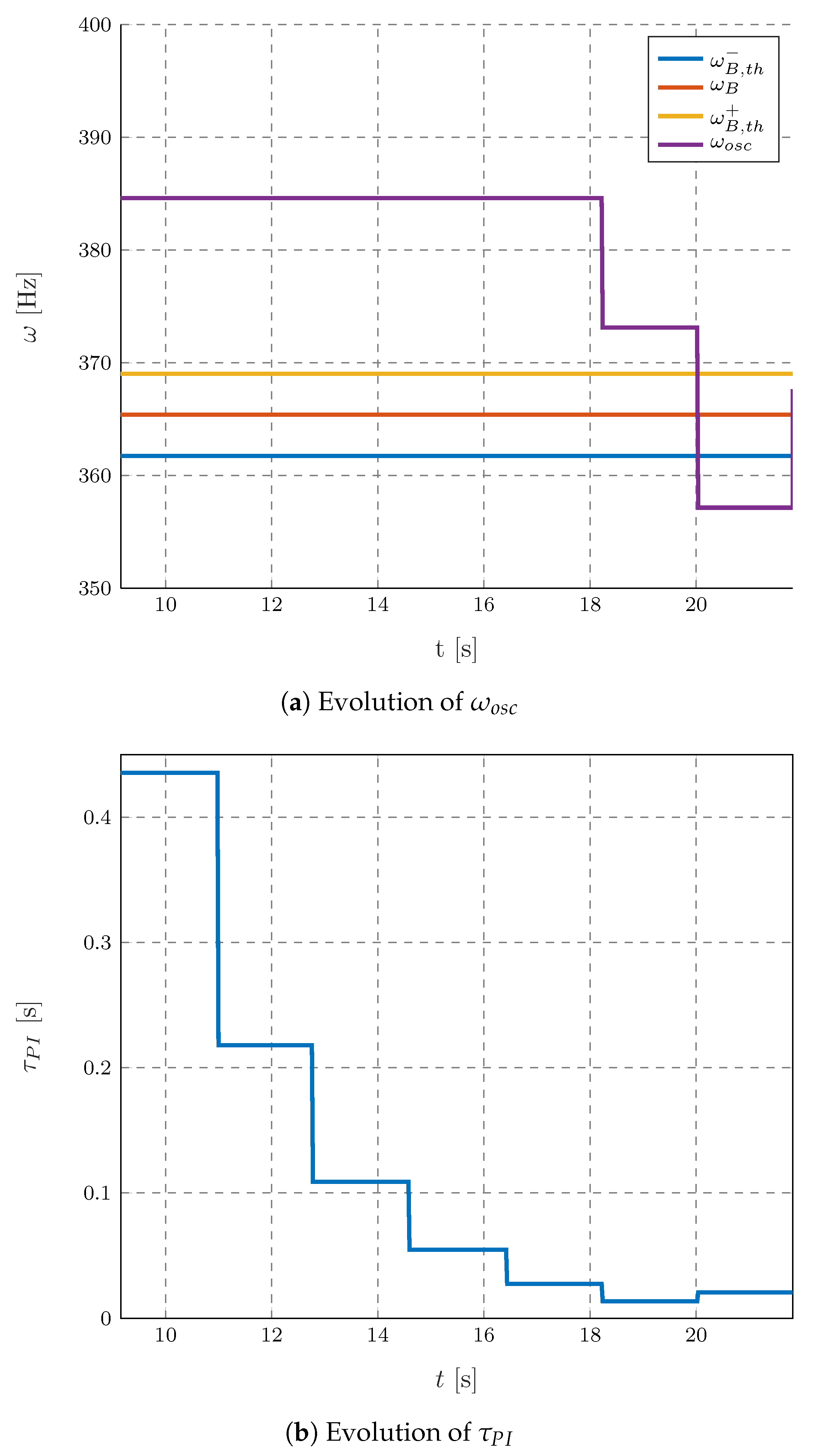
After measurement, the target value of can be decreased, the LPF filter and were updated accordingly, and a new perturbation is applied. Figure 5 shows the evolution of the target and the measurement during the search of the MAB. Each horizontal segment coincides with a perturbation of the system and a measurement of the relative .
After the measure, is compared with . Since , the phase lag due to the PI at the observed frequency is at its minimum. is the maximum oscillation frequency reachable from the given system with the LPF designed in a function of the actual . If , the requested dynamic specifications are impossible to achieve with a simple PI. Thus, is gradually decreased until . From this final value, the procedure can start to tune the PI in a function of the obtained and desired .
The procedure continues repeating Algorithm 2 along each current axis and for different values of the current offset. The autotuning performed imposing the MAB achieved in simulation with a phase margin of 65 gives the results reported in Figure 6.
Comparing the two figures, it is possible to see that the procedure starts with a high value of which is gradually decreased in order to achieve the desired phase margin at the given bandwidth. During the initial transient of the procedure, is so high that its variation does not produce a perceivable phase lag. Thus, even if is changed the measure of remains invariant. When moves near one decade below , it starts to have some effect on the total phase lag of the system and so on the oscillation frequency. In order to speed up the procedure, two thresholds on the target are fixed which are placed at . Once is within these boundaries, the time constant of PI is assumed to be tuned. This condition corresponds to the final instant of the figures. The measure of is achieved with .
Further results were obtained experimentally and are reported in the next section.
5. Experimental Results
The experimental results implementing all the design hints discussed above are reported hereafter. The test rig was composed by a SynR motor and an industrial inverter whose nameplate data are reported in Table 1. The drive was controlled by a dSpace MicroLabBox system. The same parameters as in the simulation tests were chosen for the autotuning procedure.
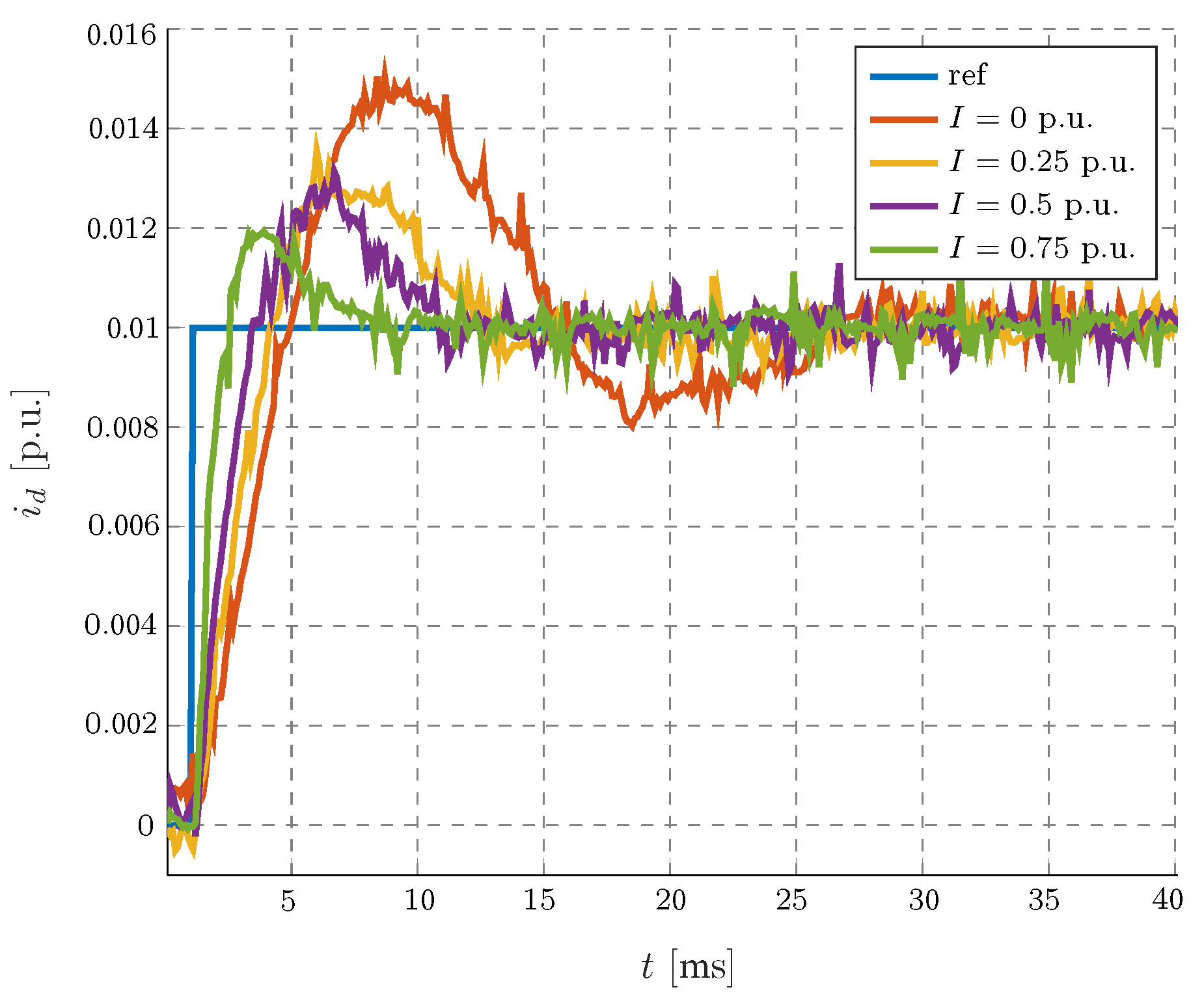
In order to demonstrate the necessity to perform several tunings for different levels of current, a first test was performed. The current step response along the d axis was analyzed. The relative controller was tuned through our autotuning technique imposing a bandwidth of and a phase margin of 65. Taking in mind that the motor dynamics change according to the magnetic saturation level the PI block was precautionarily tuned at of the nominal current. For lower currents, the dynamics become less acceptable, but the stability of the system is maintained. These concepts are demonstrated experimentally in Figure 7.
Maintaining the same PI a step of current with amplitude ( p.u.) is performed at different levels of current (0 p.u., p.u., p.u., p.u.). The time response corresponds to the desired bandwidth only when the current offset p.u. at which the PI was designed. For other values, the performance decreases noticeably.
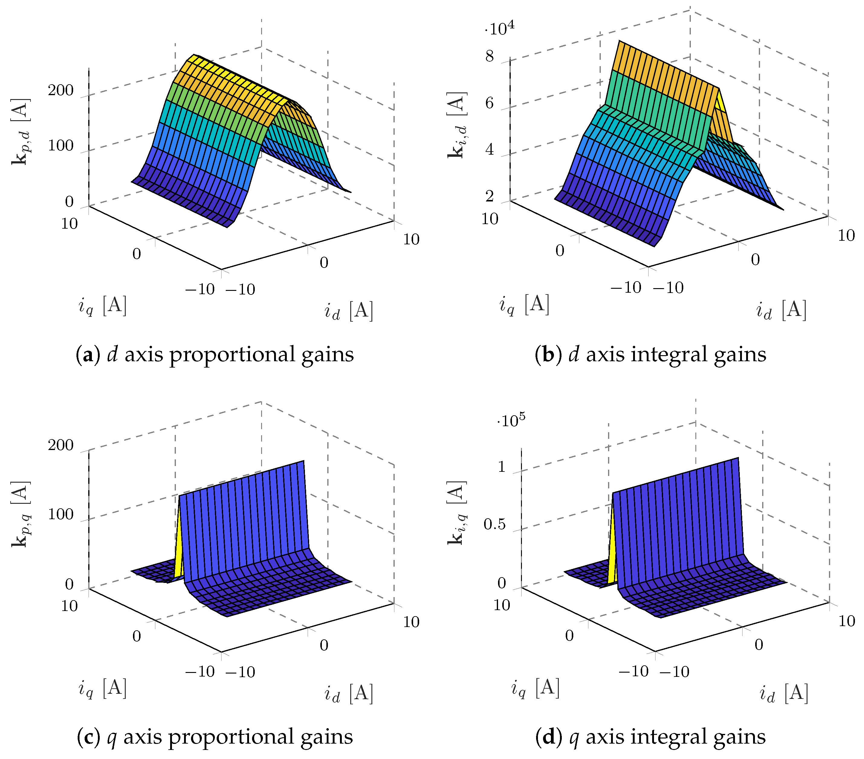
Keeping the same control targets, the autotuning was repeatedly performed along the d and q axes for different levels of currents starting from 0 p.u. to p.u. by steps of p.u. The obtained gains along the axes are so repeated (assuming absence of cross-coupling) in order to map the whole operating range of the motor. The results obtained are reported in Figure 8.
6. Discussion of the Results
The shapes of the maps reported in Figure 8 resemble those of the differential inductances reported in Figure 1. In other words, the results of Figure 8 show qualitatively how the gains change due to the magnetic iron saturation.
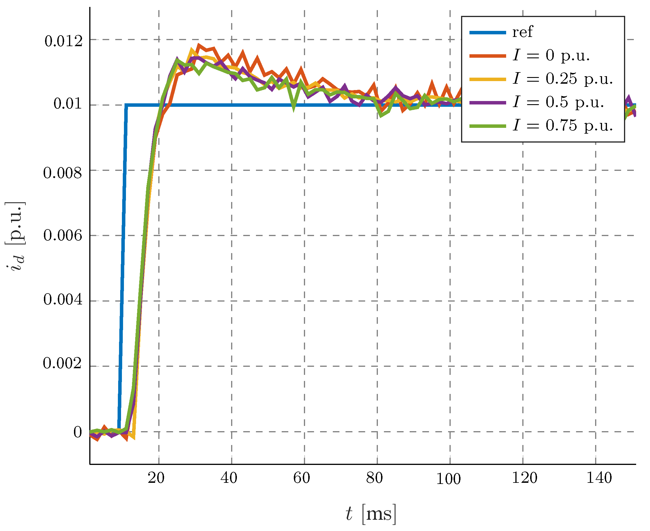
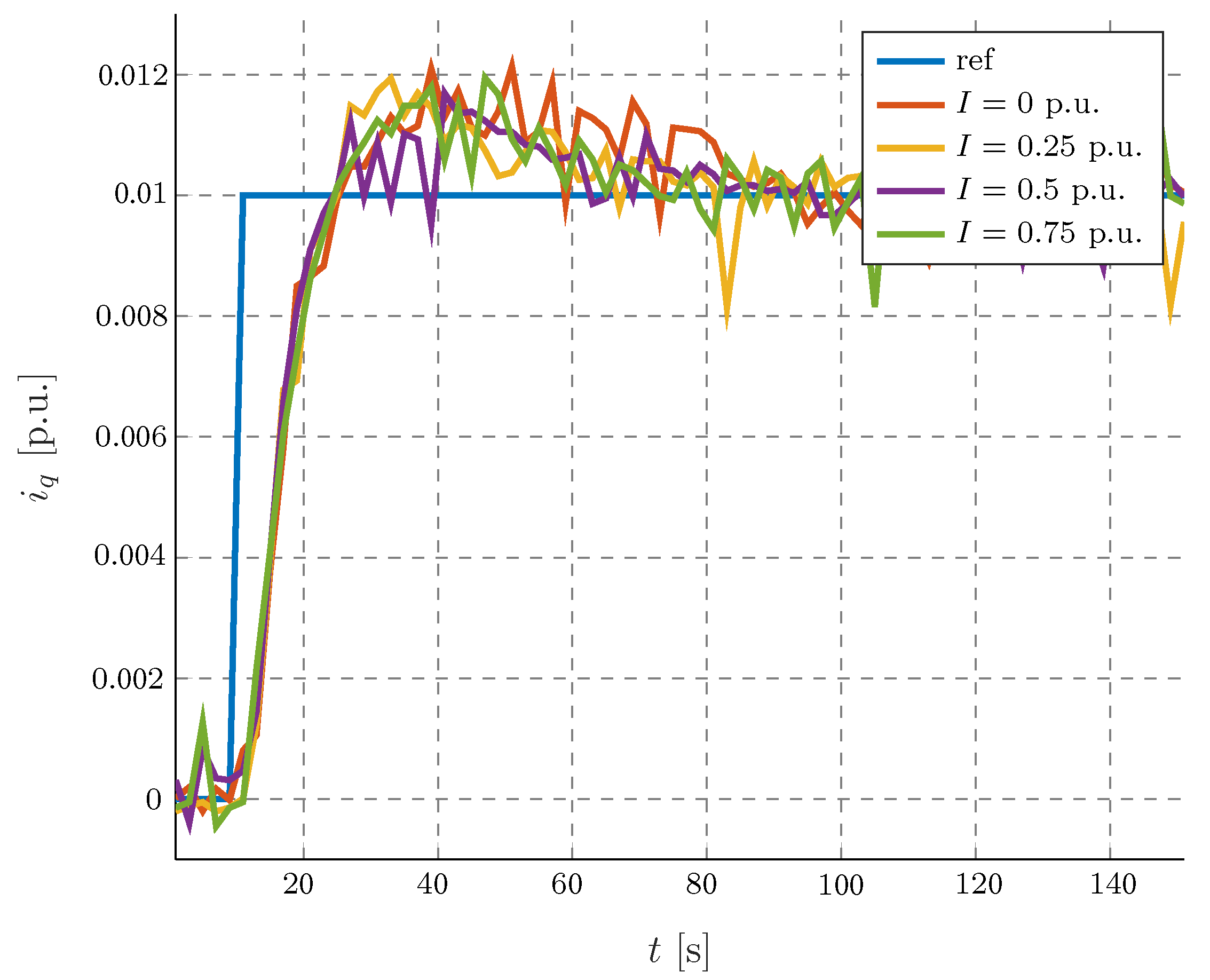
The detrimental effects of iron saturation lead to the results of Figure 7, where the dynamic performance of the current control loop cannot be satisfactory. However, the results of the proposed procedure, in turn the gains reported in Figure 8, can be fruitfully adopted to get fast and repeatable adequate dynamic responses in the whole operating region. In other words, a constant control bandwidth has to be guaranteed regardless of the actual working point of the motor. The results reported in Figure 9 and Figure 10 suggest that this is possible by adopting the variable PI gains obtained by the proposed procedure. Finally, it is possible to infer from Figure 9 and Figure 10 how the gains calculated at different levels of current effectively facilitates guaranteeing the same control dynamic even under various saturations of the motor.
7. Conclusions
In conclusion, an automatic method for PI autotuning of a SynR motor is presented in this paper. The proposed procedure rests on the relay autotuning method, but its application has been tailored to nonlinear SynR motors, whereas prior research efforts were dedicated to permanent magnet synchronous motors with linear flux–current relationship. No information about the motor parameters values is needed, thus keeping the model-free characteristic of the relay autotuning method. The procedure is effective and it can be easily implemented and industrialized. According to the typical industrial specifications, the autotuning does not only tune the system to have a certain dynamics, but it can also find the maximum performance achievable with a PI controller through the whole operating region of the motor. Furthermore, the rotor remains at standstill throughout the whole autotuning procedure. The procedure is validated using both simulation and experimental results, which demonstrate the importance of having variable gain PI controllers for achieving satisfactory dynamics in the whole operating region.
Author Contributions
All authors have contributed equally to this work. All authors have read and agreed to the published version of the manuscript. D.P. performed the Formal analysis, Methodology, Software and Writing – original draft; F.T. contributed to Validation and Visualization; M.Z. supervised the research Project administration, contributed to review and editing.
Funding
This research received no external funding..
Conflicts of Interest
The authors declare no conflict of interest.
References
- Ortombina, L.; Pasqualotto, D.; Tinazzi, F.; Zigliotto, M. Magnetic Model Identification for Synchronous Reluctance Motors Including Transients. In Proceedings of the 2019 IEEE Energy Conversion Congress and Exposition (ECCE), Baltimore, MD, USA, 29 September–3 October 2019; pp. 3196–3202. [Google Scholar]
- Wei, M.; Liu, T. Design and Implementation of an Online Tuning Adaptive Controller for Synchronous Reluctance Motor Drives. IEEE Trans. Ind. Electron. 2013, 60, 3644–3657. [Google Scholar] [CrossRef]
- Daryabeigi, E.; Mirzaei, A.; Abootorabi Zarchi, H.; Vaez-Zadeh, S. Enhanced Emotional and Speed Deviation Control of Synchronous Reluctance Motor Drives. IEEE Trans. Energy Convers. 2019, 34, 604–612. [Google Scholar] [CrossRef]
- Antonello, R.; Ortombina, L.; Tinazzi, F.; Zigliotto, M. Advanced current control of synchronous reluctance motors. In Proceedings of the 2017 IEEE 12th International Conference on Power Electronics and Drive Systems (PEDS), Honolulu, HI, USA, 12–15 December 2017; pp. 1037–1042. [Google Scholar]
- Hackl, C.M.; Kamper, M.J.; Kullick, J.; Mitchell, J. Current control of reluctance synchronous machines with online adjustment of the controller parameters. In Proceedings of the 2016 IEEE 25th International Symposium on Industrial Electronics (ISIE), Santa Clara, CA, USA, 8–10 June 2016; pp. 153–160. [Google Scholar]
- Wiedemann, S.; Kennel, R.M. Self-Commissioning of the Current Control Loop in AC Drives. In Proceedings of the PCIM Europe 2018: International Exhibition and Conference for Power Electronics, Intelligent Motion, Renewable Energy and Energy Management, Nuremberg, Germany, 5–7 June 2018; pp. 1–8. [Google Scholar]
- Åström, K.; Hägglund, T. Automatic tuning of simple regulators with specifications on phase and amplitude margins. Automatica 1984, 20, 645–651. [Google Scholar] [CrossRef] [Green Version]
- Levy, S.; Korotkin, S.; Hadad, K.; Ellenbogen, A.; Arad, M.; Kadmon, Y. PID autotuning using relay feedback. In Proceedings of the 2012 IEEE 27th Convention of Electrical and Electronics Engineers in Israel, Eilat, Israel, 14–17 November 2012; pp. 1–4. [Google Scholar]
- Mattavelli, P.; Tubiana, L.; Zigliotto, M. Simple control autotuning for PMSM drives based on feedback relay. In Proceedings of the 2005 European Conference on Power Electronics and Applications, Dresden, Germany, 11–14 September 2005; pp. 1–10. [Google Scholar]
- Armando, E.; Bojoi, R.I.; Guglielmi, P.; Pellegrino, G.; Pastorelli, M. Experimental Identification of the Magnetic Model of Synchronous Machines. IEEE Trans. Ind. Appl. 2013, 49, 2116–2125. [Google Scholar] [CrossRef]
- Gaeta, A.; Zanchetta, P.; Tinazzi, F.; Zigliotto, M. Advanced self-commissioning and feed-forward compensation of inverter nonlinearities. In Proceedings of the 2015 IEEE International Conference on Industrial Technology (ICIT), Seville, Spain, 17–19 March 2015; pp. 610–616. [Google Scholar]
- Park, Y.; Sul, S. A Novel Method Utilizing Trapezoidal Voltage to Compensate for Inverter Nonlinearity. IEEE Trans. Power Electron. 2012, 27, 4837–4846. [Google Scholar]
- Bedetti, N.; Calligaro, S.; Petrella, R. Self-Commissioning of Inverter Dead-Time Compensation by Multiple Linear Regression Based on a Physical Model. IEEE Trans. Ind. Appl. 2015, 51, 3954–3964. [Google Scholar]
Figure 1.
Differential inductance maps of the SynR motor under test calculated from magnetic maps as in [10].
Figure 1.
Differential inductance maps of the SynR motor under test calculated from magnetic maps as in [10].

Figure 2.
Relay feedback-based autotuning system.

Figure 3.
Current waveform during a perturbation of the system.

Figure 4.
The current , output of the relay, and output of the LPF.

Figure 5.
Evolution of the target and the oscillation measurement during the search of the MAB.

Figure 6.
and signals during autotuning along axis d with a current offset .

Figure 7.
Step responses at different levels of current and PI with constant gains.

Figure 8.
Adaptive PI gains obtained through the proposed autotuning technique.

Figure 9.
Step responses along the d-axis for different current levels with the adaptive PI maps obtained through the proposed autotuning technique with and .
Figure 9.
Step responses along the d-axis for different current levels with the adaptive PI maps obtained through the proposed autotuning technique with and .

Figure 10.
Step responses along the q-axis for different current levels with the adaptive PI maps obtained through the proposed autotuning technique with and .
Figure 10.
Step responses along the q-axis for different current levels with the adaptive PI maps obtained through the proposed autotuning technique with and .


Table 1.
Inverter and SynR motor data.
| Nominal current () | |
| Nominal speed () | |
| Nominal torque () | |
| Number of pole pairs (p) | 2 |
| Stator resistance (R) | |
| Inverter switching period () |
Table 2.
Autotuning parameters.
| Relay hysteresis () | |
| Oscillation amplitude (a) | |
| Initial (unfeasible) bandwidth specification |
© 2020 by the authors. Licensee MDPI, Basel, Switzerland. This article is an open access article distributed under the terms and conditions of the Creative Commons Attribution (CC BY) license (http://creativecommons.org/licenses/by/4.0/).
Share and Cite
MDPI and ACS Style
Pasqualotto, D.; Tinazzi, F.; Zigliotto, M. Model-Free Current Loop Autotuning for Synchronous Reluctance Motor Drives. Automation 2020, 1, 33-47. https://0-doi-org.brum.beds.ac.uk/10.3390/automation1010003
AMA Style
Pasqualotto D, Tinazzi F, Zigliotto M. Model-Free Current Loop Autotuning for Synchronous Reluctance Motor Drives. Automation. 2020; 1(1):33-47. https://0-doi-org.brum.beds.ac.uk/10.3390/automation1010003
Chicago/Turabian StylePasqualotto, Dario, Fabio Tinazzi, and Mauro Zigliotto. 2020. "Model-Free Current Loop Autotuning for Synchronous Reluctance Motor Drives" Automation 1, no. 1: 33-47. https://0-doi-org.brum.beds.ac.uk/10.3390/automation1010003