Semilocal Convergence of the Extension of Chun’s Method

Abstract

In this work, we use the technique of recurrence relations to prove the semilocal convergence in Banach spaces of the multidimensional extension of Chun’s iterative method. This is an iterative method of fourth order, that can be transferred to the multivariable case by using the divided difference operator. We obtain the domain of existence and uniqueness by taking a suitable starting point and imposing a Lipschitz condition to the first Fréchet derivative in the whole domain. Moreover, we apply the theoretical results obtained to a nonlinear integral equation of Hammerstein type, showing the applicability of our results.

1. Introduction

In this paper, we focus on solving nonlinear systems of equations, that is $F\left(x\right)=0$ where $F:\Omega \subset X⟶Y$, is a nonlinear continuous and twice differentiable Fréchet operator in an open convex set $\Omega$, and X and Y Banach spaces. It is well known that these kind of problems usually can not be solved analytically and then we use iterative methods for approximating the solution.

One of the best known iterative method is Newton’s method, [1], whose iterative function is given by

$$x_{k+1}=x_k-{\Gamma }_{k}F\left(x_k\right)$$

with ${\Gamma }_k={\left[F^{\prime }\left(x_k\right)\right]}^{-1}$ for $k=0,1,2,\dots$, being $x_0$ the starting point. The simplicity of its iterative expression and second order of convergence confers to Newton’s method a very useful efficiency in many applied problems.

Nevertheless, in the recent years, one can find in the literature a great variety of iterative methods that can reach higher convergence order and better efficiency than Newton’s method, see [2,3] and the references therein. In these texts, we can see the study about the convergence order of the methods always related with the computational efficiency reached.

However, it is also important to complete the study with theoretical results of semilocal convergence of these iterative methods, not only to prove the convergence of the iterates sequence, also because we can demonstrate the existence of solutions for a particular problem. This can be of particular interest in some applied problems, where the existence of solution is not trivial. Moreover, we obtain uniqueness domains for the solutions, see [4,5] and the references therein.

The semilocal convergence ball, $B(x_0,R)$ gives us a neighborhood in the operators domain centered in the starting guess where the sequence of iterates $x_k$ with $k=1,2,\dots$ remains. Moreover, it is proven that this sequence converges to $x^{*}\in \overline{B(x_0,R)}$ and it is verified that $F\left(x^{*}\right)=0,$ so it is called the existence domain for the solution. Then, the study of the domain of uniqueness completes the analysis.

Specially relevant are the works on the convergence of derivative-free Banach spaces (as can be seen in [3,6]). Different authors have devoted their efforts to this task, either on Steffensen’s method [7], Steffensen-type [8,9,10], or the secant scheme [11,12,13]. In those problems where the nonlinear operator F is not differentiable, we can approximate the derivatives by divided differences using a numerical derivation formula, and so, one can introduce iterative processes that use divided differences instead of derivatives. Let us consider the operator $[u,v;F]:\Omega \subset X⟶Y$, $u,v\in \Omega ,$ with $u\ne v$, it is a first-order divided difference [1,14,15] satisfying

$$[u,v;F]\in \mathcal{L}(X,Y)\mathrm{and}[u,v;F](u-v)=F\left(u\right)-F\left(v\right),$$

(1)

where $\mathcal{L}(X,Y)$ is the set of bounded linear operators between X and Y. By using this approximation for the derivative, we find in the literature the so called derivative free iterative methods, see [4,16]. But, as it was stated originally in [17,18], the divided difference operator can be used for extending an iterative method defined for the scalar case (without direct extension) into a vectorial iterative method. Our aim is to analyze the fourth order of convergence extension of Chun’s method (see [17]), whose iterative scheme is

$$x_{k+1}=y_k-\left(3I-2{\Gamma }_k[x_k,y_k;F]\right){\Gamma }_{k}F\left(y_k\right),$$

(2)

where $y_k=x_k-{\Gamma }_{k}F\left(x_k\right)$ is the Newton’s step, $[x,y;F]$ is the divided difference operator, and ${\Gamma }_k={\left[F^{\prime }\left(x_k\right)\right]}^{-1}$.

This method was introduced and analyzed in [17], but now, we are interested in its semilocal convergence study. For this purpose we use the recurrence relation technique. This method was defined by Candela et al. in [19,20] as a system of four real sequences for the third-order Halley’ and Chebyshev’s schemes. Hernández-Verón et al. simplified this technique, establishing a system of as many scalar sequences as the order of convergence of the iterative method minus one (see [21,22,23,24]).

The rest of the paper is organized as follows: in Section 2 we describe the recurrence relations and the properties needed to prove the semilocal convergence of the fourth order method, which is developed in Section 3. Next, Section 4 is devoted to the application of the theoretical results obtained to a Hammerstein integral equation, with very good results. Finally, in Section 5 we draw some final remarks.

2. Recurrence Relations

Let X and Y be Banach spaces and let $F:\Omega \subseteq X\to Y$ be a twice differentiable nonlinear Fréchet operator in an open $\Omega$.

The iterative scheme of the fourth order Chun’s method extended to multidimensional case is

$$x_{k+1}=y_k-\left(3I-2{\Gamma }_k[x_k,y_k;F]\right){\Gamma }_{k}F\left(y_k\right),$$

(3)

where $y_k=x_k-{\Gamma }_{k}F\left(x_k\right)$ is the Newton’s step, $[x,y;F]$ is the divided difference operator, and ${\Gamma }_k={\left[F^{\prime }\left(x_k\right)\right]}^{-1}$.

Let us assume that the inverse of the Jacobian matrix of the system in the first iteration, ${\Gamma }_0\in \mathcal{L}(Y,X)$, exists in $x_0\in \Omega$, where $\mathcal{L}(Y,X)$ is the set of linear operators from Y to X.

Moreover, in order to obtain the semilocal convergence result for this iterative method, Kantorovich conditions are assumed:

(C₁)

$\parallel {\Gamma }_0\parallel \le \beta$,

(C₂)

$\parallel {\Gamma }_{0}F\left(x_0\right)\parallel \le \eta$,

(C₃)

$\parallel F^{\prime }\left(x\right)-F^{\prime }\left(y\right)\parallel \le K\parallel x-y\parallel$,

where K, $\beta$, $\eta$ are non-negative real numbers. For the sake of simplicity, we denote $a_0=K\beta \eta$ and define the sequence

$$a_{n+1}=a_{n}f{\left(a_n\right)}^{2}g\left(a_n\right),$$

(4)

where we use the following auxiliary functions

$$h\left(x\right)=x+x^2,$$

(5)

$$f\left(x\right)={\displaystyle \frac{1}{1-x(1+\frac{1}{2}h\left(x\right)),}}$$

(6)

and

$$g\left(x\right)=\frac{x}{2}+\frac{1}{2}\left(\frac{x}{\eta }+1\right)h\left(x\right)+\frac{x}{8}{\left(h\left(x\right)\right)}^2,$$

(7)

that will play a key role for obtaining the main results of this work.

Preliminary Results

Once the needed recurrence relation and the auxiliary functions have been defined, we proceed to analyze the iterative method step by step, as the basis for the later semilocal convergence analysis.

The difference between the first two elements of the iterative sequence defined in (3) is

$$x_1-x_0=(y_0-x_0)-\left(3I-2{\Gamma }_0[x_0,y_0;F]\right){\Gamma }_{0}F\left(y_0\right).$$

(8)

The Taylor series expansion of F around $x_0$ evaluated in $y_0$ is

$$F\left(y_0\right)=F\left(x_0\right)+F^{\prime }\left(x_0\right)(y_0-x_0)+{\int }_{x_0}^{y_0}(F^{\prime }\left(x\right)-F^{\prime }\left(x_0\right))dx,$$

where the term $F\left(x_0\right)+F^{\prime }\left(x_0\right)(y_0-x_0)$ is equal to zero, since it comes from a Newton’s step. With the change $x=x_0+t(y_0-x_0)$, we get

$$F\left(y_0\right)={\int }_0^1\left(F^{\prime }(x_0+t(y_0-x_0))-F^{\prime }\left(x_0\right)\right)(y_0-x_0)dt.$$

The divided difference operator can be expressed in an integral way by means of the Genocchi-Hermite formula $[x,y;F]={\int }_0^1{F}^{\prime }(x+t(y-x))dt$, see [1]. By replacing the integral expression of $F\left(y_0\right)$ in (8),

$$\begin{array}{ccc}\hfill x_1-x_0& =& (y_0-x_0)-\left(3I-2{\Gamma }_0{\int }_0^1{F}^{\prime }(x_0+t(y_0-x_0))dt\right)\hfill \\ & & {\Gamma }_0\left({\int }_0^1\left(F^{\prime }(x_0+t(y_0-x_0))-F^{\prime }\left(x_0\right)\right)(y_0-x_0)dt\right).\hfill \end{array}$$

Then,

$$\begin{array}{ccc}\hfill x_1-x_0& =& (y_0-x_0)-3{\Gamma }_0{\int }_0^1(F^{\prime }(x_0+t(y_0-x_0))-F^{\prime }\left(x_0\right))(y_0-x_0)dt+\hfill \\ \hfill & & +2{\Gamma }_0^2{\int }_0^1{F}^{\prime }(x_0+t(y_0-x_0))dt{\int }_0^1(F^{\prime }(x_0+t(y_0-x_0))-F^{\prime }\left(x_0\right))(y_0-x_0)dt.\hfill \end{array}$$

Adding and subtracting $F^{\prime }\left(x_0\right)$ to the second integral, the terms can be grouped

$$\begin{array}{ccc}\hfill x_1-x_0& =& (y_0-x_0)-{\Gamma }_0{\int }_0^1(F^{\prime }(x_0+t(y_0-x_0))-F^{\prime }\left(x_0\right))(y_0-x_0)dt\hfill \\ \hfill & & +2{\Gamma }_0^2{\int }_0^1(F^{\prime }(x_0+t(y_0-x_0))-F^{\prime }\left(x_0\right))dt\hfill \\ & & {\int }_0^1(F^{\prime }(x_0+t(y_0-x_0))-F^{\prime }\left(x_0\right))(y_0-x_0)dt.\hfill \end{array}$$

Taking norms and applying Lipschitz condition, we get

$$\begin{array}{ccc}\hfill \parallel x_1-x_0\parallel & \le & \parallel y_0-x_0\parallel +\parallel {\Gamma }_0\parallel \frac{K}{2}\parallel y_0-x_0{\parallel }^2+2\parallel {\Gamma }_0{\parallel }^2\left[\frac{K}{2}\parallel y_0-x_0\parallel \right]\frac{K}{2}{\parallel y_0-x_0\parallel }^2\hfill \\ & \le & \eta +\beta \frac{K}{2}{\eta }^2+\frac{1}{2}{K}^2{\beta }^2{\eta }^3=\eta \left(1+\frac{1}{2}(a_0+a_0^2)\right)=\eta \left(1+\frac{1}{2}h\left(a_0\right)\right),\hfill \end{array}$$

so that

$$\parallel x_1-x_0\parallel \le \eta \left(1+\frac{h\left(a_0\right)}{2}\right),$$

(9)

where $a_0=K\beta \eta$ and $h\left(x\right)=x+x^2$.

By applying Banach’s lemma [1], one has

$$\begin{array}{ccc}\hfill \parallel I-{\Gamma }_0{F}^{\prime }\left(x_1\right)\parallel & =& \parallel {\Gamma }_0{F}^{\prime }\left(x_0\right)-{\Gamma }_0{F}^{\prime }\left(x_1\right)\parallel \hfill \\ & =& \parallel {\Gamma }_0\parallel \parallel F^{\prime }\left(x_0\right)-F^{\prime }\left(x_1\right)\parallel \hfill \\ & \le & K\beta \parallel x_1-x_0\parallel \hfill \\ & \le & K\beta \eta (1+{\displaystyle \frac{1}{2}}(a_0+a_0^2))\hfill \\ & =& a_0\left(1+{\displaystyle \frac{1}{2}}h\left(a_0\right)\right)<1.\hfill \end{array}$$

Then, as far as $a_0\left(1+\frac{1}{2}h\left(a_0\right)\right)<1$ (by taking $a_0<0.650629$), Banach’s lemma guarantees that ${\left({\Gamma }_0{F}^{\prime }\left(x_1\right)\right)}^{-1}={\Gamma }_1{\Gamma }_0^{-1}$ exists and

$$\parallel {\Gamma }_1\parallel \le \frac{1}{1-a_0(1+\frac{1}{2}{a}_0+\frac{1}{2}{a}_0^2)}\parallel {\Gamma }_0\parallel =f\left(a_0\right)\parallel {\Gamma }_0\parallel ,$$

(10)

being $f\left(x\right)={\displaystyle \frac{1}{1-x\left(1+\frac{1}{2}h\left(x\right)\right)}}$.

Now, the following bounds are proven by induction for $n\ge 1$:

(I_n)

$\parallel {\Gamma }_n\parallel \le f\left(a_{n-1}\right)\parallel {\Gamma }_{n-1}\parallel$,

(II_n)

$\parallel y_n-x_n\parallel =\parallel {\Gamma }_{n}F\left(x_n\right)\parallel \le f\left(a_{n-1}\right)g\left(a_{n-1}\right)\parallel y_{n-1}-x_{n-1}\parallel$,

(III_n)

$K\parallel {\Gamma }_n\parallel \parallel y_n-x_n\parallel \le a_n$,

(IV_n)

$\parallel x_n-x_{n-1}\parallel \le \left(1+{\displaystyle \frac{1}{2}}h\left(a_{n-1}\right)\right)\parallel y_{n-1}-x_{n-1}\parallel$.

Starting with $n=1$, ($I_1$) has been proven in (10).

(II₁):

By means of the Taylor’s expansion of $F\left(x_1\right)$ around $y_0$, we get

$$\begin{array}{ccc}\hfill F\left(x_1\right)& =& F\left(y_0\right)+F^{\prime }\left(y_0\right)(x_1-y_0)+{\int }_{y_0}^{x_1}\left(F^{\prime }\left(x\right)-F^{\prime }\left(y_0\right)\right)dx\hfill \\ & =& F\left(y_0\right)+(F^{\prime }\left(y_0\right)-F^{\prime }\left(x_0\right))(x_1-y_0)+F^{\prime }\left(x_0\right)(x_1-y_0)\hfill \\ & & +{\int }_0^1\left(F^{\prime }(y_0+t(x_1-y_0))-F^{\prime }\left(y_0\right)\right)(x_1-y_0)dt.\hfill \end{array}$$

(11)

To obtain a bound, it is necessary to calculate $x_1-y_0$. Writing the terms of the iterative Formula (3) in their integral form,

$$\begin{array}{ccc}\hfill x_1-y_0& =& -3{\Gamma }_{0}F\left(y_0\right)+2[x_0,y_0;F]{\Gamma }_0^{2}F\left(y_0\right)\hfill \\ & =& -3{\Gamma }_0{\int }_0^1(F^{\prime }(x_0+t(y_0-x_0))-F^{\prime }\left(x_0\right))(y_0-x_0))dt\hfill \\ & & +2{\Gamma }_0^2\left({\int }_0^1{F}^{\prime }(x_0+t(y_0-x_0))dt\right){\int }_0^1(F^{\prime }(x_0+t(y_0-x_0))-F^{\prime }\left(x_0\right))(y_0-x_0)dt\hfill \\ & =& -{\Gamma }_0{\int }_0^1(F^{\prime }(x_0+t(y_0-x_0))-F^{\prime }\left(x_0\right))(y_0-x_0))dt\hfill \\ & & +2{\Gamma }_0^2{\int }_0^1(F^{\prime }(x_0+t(y_0-x_0))-F^{\prime }\left(x_0\right))dt\hfill \\ & & {\int }_0^1(F^{\prime }(x_0+t(y_0-x_0))-F^{\prime }\left(x_0\right))(y_0-x_0)dt,\hfill \end{array}$$

and bounding its norm, the following inequality is obtained

$$\parallel x_1-y_0\parallel \le {\displaystyle \frac{1}{2}}K\beta {\eta }^2+{\displaystyle \frac{1}{2}}{K}^2{\beta }^2{\eta }^3={\displaystyle \frac{1}{2}}\eta a_0+{\displaystyle \frac{1}{2}}\eta a_0^2={\displaystyle \frac{1}{2}}\eta h\left(a_0\right).$$

(12)

Taking norms in (11) and replacing (12) in it, finally $\parallel F\left(x_1\right)\parallel$ is bounded

$$\parallel F\left(x_1\right)\parallel \le \frac{1}{2}K{\eta }^2+\frac{1}{2}K{\eta }^{2}h\left(a_0\right)+\frac{1}{2\beta }\eta h\left(a_0\right)+\frac{1}{8}K{\eta }^2{\left(h\left(a_0\right)\right)}^2.$$

Therefore, by applying $\left(I_1\right)$,

$$\begin{array}{ccc}\hfill \parallel y_1-x_1\parallel & =& \parallel {\Gamma }_{1}F\left(x_1\right)\parallel =f\left(a_0\right)\parallel {\Gamma }_0\parallel \parallel F\left(x_1\right)\parallel \le \hfill \\ & \le & f\left(a_0\right)\left[{\displaystyle \frac{1}{2}}{a}_0+{\displaystyle \frac{1}{2}}\left(a_0+1\right)h\left(a_0\right)+{\displaystyle \frac{1}{8}}{a}_0{\left(h\left(a_0\right)\right)}^2\right]\eta ,\hfill \end{array}$$

that is,

$$\parallel y_1-x_1\parallel =f\left(a_0\right)g\left(a_0\right)\eta \le f\left(a_0\right)g\left(a_0\right)\parallel y_0-x_0\parallel ,$$

is obtained, where

$$g\left(x\right)=\frac{x}{2}+\frac{1}{2}(x+1)h\left(x\right)+\frac{x}{8}{\left(h\left(x\right)\right)}^2.$$

(III₁):

using ($I_1$) and ($I{I}_1$),

$$K\parallel {\Gamma }_1\parallel \parallel y_1-x_1\parallel \le Kf\left(a_0\right)\parallel {\Gamma }_0\parallel f\left(a_0\right)g\left(a_0\right)\parallel y_0-x_0\parallel =a_0{\left(f\left(a_0\right)\right)}^{2}g\left(a_0\right)=a_1.$$

(IV₁):

for $n=1$ it has been proven in (9).

Taking $\left(I_n\right),\left(I{I}_n\right),\left(II{I}_n\right),\left(I{V}_n\right)$ as an inductive hypothesis for $n\ge 1$ it can be proven in a similar way that $\left(I_{n+1}\right),\left(I{I}_{n+1}\right),\left(II{I}_{n+1}\right),\left(I{V}_{n+1}\right)$ are also true and these complete the proof by induction.

3. Convergence Analysis

It is well known that to analyze the convergence of a sequence $\left\{x_n\right\}$ in a Banach space, it is necessary to prove that it is a Cauchy sequence. To get this aim, we analyze the properties of the recurrence sequence $\left\{a_n\right\}$ and the auxiliary functions $h\left(x\right)$, $f\left(x\right)$ and $g\left(x\right)$ introduced in Section 2 by giving the following preliminary results.

Lemma 1.

Let $h\left(x\right),$ $f\left(x\right)$ and $g\left(x\right)$ be defined as in (5)–(7). Then,

(i)

$f\left(x\right)$ is increasing and $f\left(x\right)>1$ for $x\in (0,0.650629)$,

(ii)

$h\left(x\right)$ and $g\left(x\right)$ are increasing for $x\in (0,0.650629)$.

Proof. 

The proof follows by elemental procedures, so we omit it. □

Lemma 2.

Let be $f\left(x\right)$ and $g\left(x\right)$ the auxiliary functions defined by (6) and (7). Then

(i)

$f\left(a_0\right)g\left(a_0\right)<1$ for $a_0<0.367826$,

(ii)

$f{\left(a_0\right)}^{2}g\left(a_0\right)<1$ for $a_0<0.300637$,

(iii)

the sequence $\left\{a_n\right\}$ is decreasing and $a_n<0.300637$ for $n\ge 0.$

Proof. 

It is straightforward that $\left(i\right)$ and $\left(ii\right)$ are satisfied. As $f{\left(a_0\right)}^{2}g\left(a_0\right)<1$, then by construction of $a_n,$ (see (4)), it is a decreasing sequence. So, $a_n<a_0\le 0.300637$, for all $n\ge 1$. □

Theorem 1.

Let X and Y be Banach spaces and let $F:\Omega \subseteq X\to Y$ be a twice differentiable Fréchet nonlinear operator in an open set Ω. Let us assume that ${\Gamma }_0={\left[F^{\prime }\left(x_0\right)\right]}^{-1}$ exists in $x_0\in \Omega$ and conditions $\left(C_1\right)-\left(C_3\right)$ are satisfied. Let be $a_0=K\beta \eta$, and assume that $a_0<0.3$. Then, if $B(x_0,R\eta )=\{x\in X:\parallel x-x_0\parallel <R\eta \}\subset \Omega$ where $R={\displaystyle \frac{1+\frac{1}{2}h\left(a_0\right)}{1-f\left(a_0\right)g\left(a_0\right)}}$, the sequence $\left\{x_n\right\}$ defined in (3) and starting in $x_0$ converges to the solution $x^{*}$ of $F\left(x\right)=0$. In that case, the iterates $\left\{x_n\right\}$ and $\left\{y_n\right\}$ are contained in $B(x_0,R\eta )$ and $x^{*}\in \overline{B(x_0,R\eta )}$. Moreover $x^{*}$ is the only solution of equation $F\left(x\right)=0$ in $B(x_0,\frac{2}{K\beta }-R\eta )\cap \Omega$.

Proof. 

By recursively applying $\left(I{V}_n\right)$, we can write

$$\begin{array}{ccc}\hfill \parallel x_{n+1}-x_n\parallel & \le & \left({\displaystyle \frac{h\left(a_n\right)}{2}}+1\right)\parallel y_n-x_n\parallel \hfill \\ & \le & \left({\displaystyle \frac{h\left(a_n\right)}{2}}+1\right)f\left(a_{n-1}\right)g\left(a_{n-1}\right)\parallel y_{n-1}-x_{n-1}\parallel \hfill \\ & \le & \cdots \le \left({\displaystyle \frac{h\left(a_n\right)}{2}}+1\right)\left[\prod _{j=0}^{n-1}f\left(a_j\right)g\left(a_j\right)\right]\parallel y_0-x_0\parallel .\hfill \end{array}$$

(13)

Then,

$$\begin{array}{cc}\hfill \parallel x_{n+m}-x_n\parallel & \le \parallel x_{n+m}-x_{n+m-1}\parallel +\parallel x_{n+m-1}-x_{n+m-2}\parallel +\cdots +\parallel x_{n+1}-x_n\parallel \\ & \le \left({\displaystyle \frac{h\left(a_{n+m-1}\right)}{2}}+1\right)\eta \prod _{j=0}^{n+m-2}f\left(a_j\right)g\left(a_j\right)\\ & +\left({\displaystyle \frac{h\left(a_{n+m-2}\right)}{2}}+1\right)\eta \prod _{j=0}^{n+m-3}f\left(a_j\right)g\left(a_j\right)\\ & +\cdots +\left({\displaystyle \frac{h\left(a_n\right)}{2}}+1\right)\eta \prod _{j=0}^{n-1}f\left(a_j\right)g\left(a_j\right).\end{array}$$

As $h\left(x\right)$ is increasing and $a_n$ decreasing, it can be stated that

$$\begin{array}{ccc}\hfill \parallel x_{n+m}-x_n\parallel & \le & \left({\displaystyle \frac{h\left(a_n\right)}{2}}+1\right)\eta \sum _{l=0}^{m-1}\left[\prod _{j=0}^{n+l-1}f\left(a_j\right)g\left(a_j\right)\right]\hfill \\ & \le & \left({\displaystyle \frac{h\left(a_n\right)}{2}}+1\right)\eta \sum _{l=0}^{m-1}{\left(f\left(a_0\right)g\left(a_0\right)\right)}^{l+n}.\hfill \end{array}$$

Moreover, by Lemmas 1 and 2, f and g are increasing and $a_n$ decreasing. So, we can use the expression for the partial sum of a geometrical series,

$$\parallel x_{n+m}-x_n\parallel \le \left({\displaystyle \frac{h\left(a_0\right)}{2}}+1\right)\frac{1-{\left(f\left(a_0\right)g\left(a_0\right)\right)}^m}{1-f\left(a_0\right)g\left(a_0\right)}{\left(f\left(a_0\right)g\left(a_0\right)\right)}^n\eta .$$

So, we conclude that $\left\{x_n\right\}$ is a Cauchy sequence if and only if $f\left(a_0\right)g\left(a_0\right)<1$ (Lemma 2).

For $n=0$,

$$\parallel x_m-x_0\parallel \le \left({\displaystyle \frac{h\left(a_0\right)}{2}}+1\right)\frac{1-{\left(f\left(a_0\right)g\left(a_0\right)\right)}^m}{1-f\left(a_0\right)g\left(a_0\right)}\eta \le R\eta ,$$

and by taking $m\to \infty$, we get the radius of convergence $R\eta ={\displaystyle \frac{1+\frac{1}{2}h\left(a_0\right)}{1-f\left(a_0\right)g\left(a_0\right)}}\eta$.

To prove that $x^{*}$ is a solution $F\left(x\right)=0$ we start bounding $\parallel F^{\prime }\left(x_n\right)\parallel$,

$$\begin{array}{ccc}\hfill \parallel F^{\prime }\left(x_n\right)\parallel & \le & \parallel F^{\prime }\left(x_0\right)\parallel +\parallel F^{\prime }\left(x_n\right)-F^{\prime }\left(x_0\right)\parallel \hfill \\ & \le & \parallel F^{\prime }\left(x_0\right)\parallel +K\parallel x_n-x_0\parallel \hfill \\ & \le & \parallel F^{\prime }\left(x_0\right)\parallel +KR\eta .\hfill \end{array}$$

Then, from (13),

$$\begin{array}{ccc}\hfill \parallel F\left(x_n\right)\parallel & \le & \parallel F^{\prime }\left(x_n\right)\parallel \parallel x_n-x_0\parallel \hfill \\ & \le & \parallel F^{\prime }\left(x_n\right)\parallel \left({\displaystyle \frac{h\left(a_n\right)}{2}}+1\right)\left[\prod _{j=0}^{n-1}f\left(a_j\right)g\left(a_j\right)\right]\eta ,\hfill \end{array}$$

as h, f and g are increasing functions and $a_n$ is a decreasing sequence,

$$\parallel F\left(x_n\right)\parallel \le \parallel F^{\prime }\left(x_n\right)\parallel \left({\displaystyle \frac{h\left(a_n\right)}{2}}+1\right){\left(f\left(a_0\right)g\left(a_0\right)\right)}^n\eta .$$

Taking into account that $\parallel F^{\prime }\left(x_n\right)\parallel$ is bounded and ${\left(f\left(a_0\right)g\left(a_0\right)\right)}^n$ tends to zero when $n\to \infty$, we conclude that $\parallel F\left(x_n\right)\parallel \to 0$. As F is continuous in $\Omega$, then $F\left(x^{*}\right)=0$.

Finally, the uniqueness of $x^{*}$ in $B\left(x_0,\frac{2}{K\beta }-R\eta \right)\cap \Omega$ is going to be proven. We assume that $y^{*}$ is another solution of $F\left(x\right)=0$ in $B(x_0,\frac{2}{K\beta }-R\eta )\cap \Omega$, and let us prove that $x^{*}=y^{*}$. Starting with the Taylor series of F around $x^{*}$,

$$F\left(x\right)=F\left(x^{*}\right)+{\int }_0^1{F}^{\prime }(x^{*}+t(x-x^{*}))(x-x^{*})dt,$$

then,

$$F\left(y^{*}\right)=F\left(x^{*}\right)+{\int }_0^1{F}^{\prime }(x^{*}+t(y^{*}-x^{*}))(y^{*}-x^{*})dt,$$

so that

$$0=F\left(y^{*}\right)-F\left(x^{*}\right)=(y^{*}-x^{*}){\int }_0^1{F}^{\prime }(x^{*}+t(y^{*}-x^{*}))dt.$$

In order to guarantee that $y^{*}-x^{*}=0$ it is necessary to prove that operator ${\int }_0^1{F}^{\prime }(x^{*}+t(y^{*}-x^{*}))dt$ is invertible. Applying hypothesis $\left(C_3\right)$,

$$\begin{array}{ccc}\hfill \parallel {\Gamma }_0\parallel {\int }_0^1\parallel F^{\prime }(x^{*}+t(y^{*}-x^{*}))-F^{\prime }\left(x_0\right)\parallel dt& \le & K\beta {\int }_0^1\parallel x^{*}+t(y^{*}-x^{*})-x_0\parallel dt\hfill \\ & \le & K\beta {\int }_0^1\left((1-t)\parallel x-x_0\parallel +t\parallel y^{*}-x_0\parallel \right)dt\hfill \\ & <& \frac{K\beta }{2}\left(R\eta +\frac{2}{K\beta }-R\eta \right)=1.\hfill \end{array}$$

Therefore, Banach’s lemma guarantees that the operator is invertible, so $y^{*}=x^{*}$ and the proof is finished. □

4. Numerical Experiments

Hammerstein’s integral equation appears in nonlinear physical phenomena, such as the dynamics of electromagnetic fluids, in the reformulation of contour problems with nonlinear boundary conditions of the Hammerstein type, etc. See, for instance, [25] or [26].

So, in order to show the applicability of the theoretical results, we apply the obtained results for solving the following Hammerstein type integral equation,

$$x\left(s\right)=1+{\int }_0^{1}G(s,t)x{\left(t\right)}^{2}dt,s\in [0,1],t\in [0,1],$$

(14)

where $x\in C(0,1)$, $t\in [0,1]$ with kernel $G(s,t)=\left\{\begin{array}{c}(1-s)t,t\le s,\hfill \\ s(1-t),s<t.\hfill \end{array}\right.$

To solve Equation (14) we transform it into a system of nonlinear equations through a discretization process. We approximate the integral appearing in (14) by using Gauss-Legendre quadrature,

$${\int }_0^{1}h\left(t\right)dt\approx \sum _{i=1}^m{w}_{i}h\left(t_i\right),$$

(15)

being $t_i$ and $w_i$ the nodes and the weights of the Gauss-Legendre polynomial. Denoting the approximation of $x\left(t_i\right)$ as $x_i$, $i=1,2,\dots ,m$, then we estimate (14) with the system of nonlinear equations

$$x_i=1+\sum _{j=1}^m{a}_{ij}{x}_j^2,i=1,2,\dots ,m$$

(16)

where $a_{ij}=\left\{\begin{array}{c}{w}_j{t}_j(1-t_i),j\le i\\ w_j{t}_i(1-t_j),j>i.\end{array}\right.$

The system can be rewritten as

$$\begin{array}{ccc}\hfill F\left(x\right)& =& x-1-A{v}_x,v_x={(x_1^2,x_2^2,\dots ,x_m^2)}^T,\hfill \\ \hfill F^{\prime }\left(x\right)& =& I-2AD\left(x\right),D\left(x\right)=diag(x_1,x_2,\dots ,x_m),\hfill \end{array}$$

where F is a nonlinear operator in the Banach space $R^m$, and $F^{\prime }$ is its Fréchet derivative in $\mathcal{L}(R^m,R^m).$ We will use the extension of Chun’s method introduced in (3) to solve the nonlinear system.

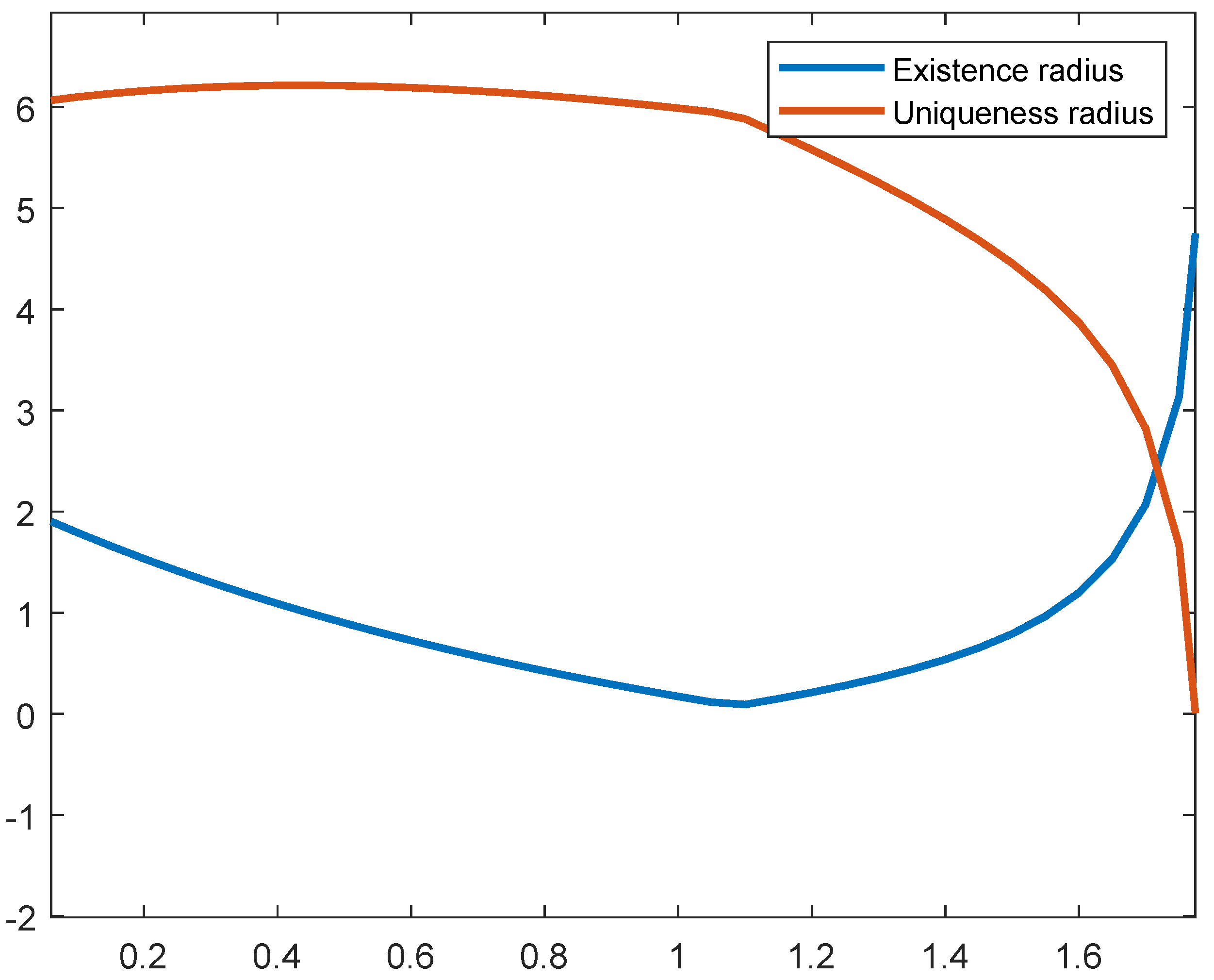
Taking $x_0={(1.7,1.7,\dots ,1.7)}^T$, $m=8$ and the infinity norm, we get

$$\begin{array}{ccc}\hfill \parallel {\Gamma }_0\parallel \le \beta ,& \beta & \approx 1.6550,\hfill \\ \hfill \parallel {\Gamma }_{0}F\left(x_0\right)\parallel \le \eta ,& \eta & \approx 0.6927,\hfill \\ \hfill \parallel F^{\prime }\left(x\right)-F^{\prime }\left(y\right)\parallel \le k\parallel x-y\parallel ,& k& \approx 0.2471,\hfill \\ \hfill a_0=k\beta \eta ,& a_0& \approx 0.2833.\hfill \end{array}$$

The convergence conditions are met and consequently the method can be applied to the system. In addition, by Theorem 1, we guarantee the existence of the solution in $B(x_0,2.0725)$, and its uniqueness in $B(x_0,2.8181)$. In

Table 1. Parameters of (16) for different initial estimations.

${{\mathit{x}}_0}_{\mathit{i}}$	$\mathit{\beta }$	$\mathit{\eta }$	${\mathit{a}}_0$	${\mathit{R}}_{\mathit{e}}$	${\mathit{R}}_{\mathit{u}}$
0	1.0000	1.0000	0.2471	2.0825	6.0108
0.2	1.0516	0.8465	0.2200	1.5346	6.1614
0.4	1.1080	0.6864	0.1879	1.0901	6.2142
0.6	1.1699	0.5189	0.1500	0.7256	6.1925
0.8	1.2380	0.3428	0.1049	0.4238	6.1134
1.0	1.3134	0.1567	0.0509	0.1720	5.9899
1.2	1.3973	0.1879	0.0649	0.2123	5.5796
1.4	1.4912	0.3889	0.1433	0.5380	4.8892
1.6	1.5969	0.5911	0.2333	1.1986	3.8694

and in Figure 1, we show the existence radius, $R_e$, and the uniqueness radius, $R_u$ for different values of the initial estimation vector $x_0$, with equal components. Let us remark that, for ${x_0}_i>1.77$, $i=1,2,\dots ,8$, convergence conditions are not satisfied and, therefore, the convergence is not guaranteed.

The approximated solution of the system (16) after 5 iterations of multidimensional Chun’s method taking $x_0={(1.7,1.7,\dots ,1.7)}^T$ and as stopping criterium $\parallel x_n-x_{n-1}{\parallel }_{\infty }<{10}^{-180}$ or $\parallel F\left(x_n\right){\parallel }_{\infty }<{10}^{-180}$, can be seen in

Table 2. Numerical solution of (16).

i	1	2	3	4	5	6	7	8
$x_i^{*}$	1.0122…	1.0584…	1.1181…	1.1598…	1.1598…	1.1181…	1.0584…	1.0122…

. The software used is MATLAB 2019b and the processor used has been Intel Core(TM) i7-9700 CPU @ 3.00 GHz with 32 GB of RAM. Variable precision arithmetics has been used in the calculations with 2000 digits of mantissa. The approximated computational order of convergence (ACOC) [27]

$$\rho =\frac{ln\frac{\parallel x_{n+1}-x_n{\parallel }_{\infty }}{\parallel x_n-x_{n-1}{\parallel }_{\infty }}}{ln\frac{\parallel x_n-x_{n-1}{\parallel }_{\infty }}{\parallel x_{n-1}-x_{n-2}{\parallel }_{\infty }}},\mathrm{for} \mathrm{each} n=2,3,\dots$$

(17)

is also calculated.

As expected, the method converges to the solution if the Kantorovich conditions are met, we obtain the same solution with any initial estimation of Table 1. As can be observed in

Table 3. Numerical results extension of Chun’s method with different initial estimations.

${{\mathit{x}}_0}_{\mathit{i}}$	iter	$\parallel {\mathit{x}}_{\mathit{n}}-{\mathit{x}}_{\mathit{n}-1}{\parallel }_{\mathit{\infty }}$	$\parallel \mathit{F}\left({\mathit{x}}_{\mathit{n}}\right){\parallel }_{\mathit{\infty }}$	$\mathit{\rho }$
0.2	5	$5.2749\times {10}^{-189}$	$9.396\times {10}^{-757}$	4.0
0.4	5	$2.9207\times {10}^{-211}$	$8.8316\times {10}^{-846}$	4.0
0.6	5	$9.5406\times {10}^{-242}$	$1.0055\times {10}^{-967}$	4.0
0.8	5	$2.2172\times {10}^{-288}$	$1.7003\times {10}^{-1008}$	4.0
1.0	5	$4.7315\times {10}^{-381}$	$1.8738\times {10}^{-1008}$	4.0
1.2	5	$1.28\times {10}^{-455}$	$3.258\times {10}^{-1823}$	4.0
1.4	5	$9.6618\times {10}^{-300}$	$1.0576\times {10}^{-1199}$	4.0
1.6	5	$4.943\times {10}^{-231}$	$7.2453\times {10}^{-925}$	4.0

, by changing the initial estimation (with equal components ${x_0}_i$, $i=1,2,\dots ,8$), the number of iterations needed to converge to the unique root is always 5, the computational order of convergence $\rho$ fits exactly the theoretical order of convergence and the estimations of the error, as it is intended, are lower as closer are initial guesses to the root.

This kind of semilocal convergence demonstrations that guarantee the existence and uniqueness of the solution under some assumptions are especially valuable in unsupervised processes where it is difficult to prove the existence of solutions.

5. Conclusions

This paper completes the study of the multidimensional extension of Chun’s fourth-order of convergence iterative method. We have analyzed the behavior of this method under Kantorovich conditions assuming a Lipschitz condition for the derivative. In these terms, we have been able to obtain the existence and uniqueness domain for the solution.

This is important not only because it gives us a theoretical proof of the iterates convergence; moreover, it is the way to prove the existence of the solution for some applied problems that cannot be solved analitically.

The theoretical study has been corroborated by solving an applied problem formulated as a nonlinear integral equation of Hammerstein type. The efficiency of this method has been proven numerically, by the calculation of high-precision approximation of the solution of an integral equation with very few iterations and fourth-order of convergence. The future work is centered in modifying the method and the corresponding semilocal convergence study for the nondifferentiable case.

References

- Ortega, J.M.; Rheinboldt, W.C. Iterative Solution of Nonlinear Equations in Several Variables; Academic Press: New York, NY, USA, 1970. [Google Scholar]
- Petković, M.S.; Neta, B.; Petković, L.D.; DŽunić, J. Multipoint Methods for Solving Nonlinear Equations; Academic Press: New York, NY, USA, 2012. [Google Scholar]
- Amat, S.; Busquier, S. Advances in Iterative Methods for Nonlinear Equations; Springer: Cham, Switzerland, 2016. [Google Scholar]
- Ezquerro, J.A.; Grau-Sánchez, M.; Hernández, M.A.; Noguera, M. A study of optimization for Steffensen-type methods with frozen divided differences. SeMA 2015, 70, 23–46. [Google Scholar] [CrossRef] [Green Version]
- Hernández-Verón, M.A.; Martínez, E.; Teruel, C. Semilocal convergence of a k-step iterative process and its application for solving a special kind of conservative problems. Numer. Algor. 2017, 6, 309–331. [Google Scholar] [CrossRef]
- Hernández, M.A.; Rubio, M.J. On the local convergence of a Newton-Kurchatov-type method for non-differentiable operators. Appl. Math. Comput. 2017, 304, 1–9. [Google Scholar] [CrossRef]
- Argyros, I.K. A new convergence theorem for Steffensen’s method on Banach spaces and applications. Southwest Pure Appl. Math. 1997, 1, 23–29. [Google Scholar]
- Alarcón, V.; Amat, S.; Busquier, S.; López, D.J. A Steffensen’s type method in Banach spaces with applications on boundary-value problems. Comput. Appl. Math. 2008, 216, 243–250. [Google Scholar] [CrossRef]
- Amat, S.; Busquier, S. A two-step Steffensen’s method under modified convergence conditions. Math. Anal. Appl. 2006, 324, 1084–1092. [Google Scholar] [CrossRef] [Green Version]
- Amat, S.; Busquier, S. On a Steffensen’s type method and its behavior for semismooth equations. Appl. Math. Comput. 2006, 177, 819–823. [Google Scholar] [CrossRef]
- Potra, F.A. On a modified Secant method. Anal. Number. Theor. Approx. 1979, 8, 203–214. [Google Scholar]
- Potra, F.A.; Ptak, V. Nondiscrete Induction and Iterative Processes; Research Notes in Mathematics 103; Pitman: Boston, MA, USA, 1984. [Google Scholar]
- Argyros, I.K.; Cordero, A.; Magreñán, Á.A.; Torregrosa, J.R. On the convergence of a damped Secant-like method with modified right hand side vector. Appl. Math. Comput. 2015, 252, 315–323. [Google Scholar]
- Balazs, M.; Goldner, G. On existence of divided differences in linear spaces. Rev. Anal. Numer. Theor. Approx. 1973, 2, 3–6. [Google Scholar]
- Grau-Sánchez, M.; Noguera, M.; Amat, S. On the approximation of derivatives using divided difference operators preserving the local convergence order of iterative methods. J. Comput. Appl. Math. 2013, 237, 363–372. [Google Scholar] [CrossRef]
- Dehghan, M.; Hajarian, M. Some derivative free quadratic and cubic convergence iterative formulas for solving nonlinear equations. Comput. Appl. Math. 2010, 29, 19–30. [Google Scholar] [CrossRef]
- Cordero, A.; García-Maimó, J.; Torregrosa, J.R.; Vassileva, M.P. Solving nonlinear problems by Ostrowski-Chun type parametric families. J. Math. Chem. 2015, 53, 430–449. [Google Scholar] [CrossRef] [Green Version]
- Abad, M.F.; Cordero, A.; Torregrosa, J.R. A family of seventh-order schemes for solving nonlinear systems. Bull. Math. Soc. Sci. Math. Roum. 2014, 57, 133–145. [Google Scholar]
- Candela, V.; Marquina, A. Recurrence relations for rational cubic models I: The Halley method. Computing 1990, 44, 169–184. [Google Scholar] [CrossRef]
- Candela, V.; Marquina, A. Recurrence relations for rational cubic models II: The Chebyshev method. Computing 1990, 45, 355–367. [Google Scholar] [CrossRef]
- Ezquerro, J.A.; Hernández, M.A. Generalized differentiability conditions for Newton’s method. IMA Numer. Anal. 2002, 22, 187–205. [Google Scholar] [CrossRef]
- Ezquerro, J.A.; Hernández, M.A. Halley’s method for operators with unbounded second derivative. Appl. Numer. Math. 2007, 57, 354–360. [Google Scholar] [CrossRef]
- Ezquerro, J.A.; Hernández, M.A. An optimization of Chebyshev’s method. Complexity 2009, 25, 343–361. [Google Scholar] [CrossRef] [Green Version]
- Cordero, A.; Hernández-Verón, M.A.; Romero, N.; Torregrosa, J.R. Semilocal convergence by using recurrence relations for a fifth-order method in Banach spaces. Comput. Appl. Math. 2015, 273, 205–213. [Google Scholar] [CrossRef]
- Hu, S.; Khavanin, M.; Zhuang, W. Integral equations arising in the kinetic theory of gases. Appl. Anal. 1989, 34, 261–266. [Google Scholar] [CrossRef]
- Maleknejad, K.; Torabi, P. Application of fixed point method for solving nonlinear Volterra-Hammerstein Integral Equation. Univ. Politeh. Buchar. Sci. Bull. Ser. A 2012, 74, 45–56. [Google Scholar]
- Cordero, A.; Torregrosa, J.R. Variants of Newton’s method using fifth-order quadrature formulas. Appl. Math. Comput. 2007, 190, 686–698. [Google Scholar] [CrossRef]
Figure 1.
Radii of existence and uniqueness for different initial estimations.