A Novel Numerical Method for Solving Fractional Diffusion-Wave and Nonlinear Fredholm and Volterra Integral Equations with Zero Absolute Error

Abstract

In this work, a new numerical method for the fractional diffusion-wave equation and nonlinear Fredholm and Volterra integro-differential equations is proposed. The method is based on Euler wavelet approximation and matrix inversion of an $M\times M$ collocation points. The proposed equations are presented based on Caputo fractional derivative where we reduce the resulting system to a system of algebraic equations by implementing the Gaussian quadrature discretization. The reduced system is generated via the truncated Euler wavelet expansion. Several examples with known exact solutions have been solved with zero absolute error. This method is also applied to the Fredholm and Volterra nonlinear integral equations and achieves the desired absolute error of $0\times {10}^{-31}$ for all tested examples. The new numerical scheme is exceptional in terms of its novelty, efficiency and accuracy in the field of numerical approximation.

1. Introduction

Fractional calculus is very useful and widely used in many applications in science, numerical computations and engineering, where the mathematical modeling of several real world problems is presented in terms of fractional differential equations, see, e.g., [1,2,3,4,5,6,7,8]. For example, the authors in [8] approximated the Caputo fractional derivative by quadratic segmentary interpolation. That raised a new approach of approximating fractional derivatives and provides some insights for a new applications where the numerical resolution of ordinary fractional differential equations is achieved.

The definition of such fractional order involves an integration represented as a non-local operator. This important feature allows to capture the previous history (memory) when calculating, for example, the time-fractional diffusion wave derivative value of a given function within certain period of time. This could not be achieved based on the classical (integer) derivative order.

The fractional diffusion-wave equation and some types of integral equations, as a mathematical models, are widely used in many physical phenomena, where the exact solution usually is difficult to obtain. Note that the authors of [9] introduced a mathematical model that intermediates between the wave, heat, and transport equations, both time and spatial variations of the corresponding dynamical law are expressed in fractional form (Caputo derivative for the time-variable and Riesz pseudo-differential operator for the spatial one), so that pure wavelike propagation is connected with pure diffusion and transport processes in unified form.

Several authors have reported the higher precision numerical solution with absolute error of ${10}^{-16}$–${10}^{-20}$ for nonlinear Volterra integral equation as in [10] and for fractional diffusion wave equation in [11]. They used the popular collocation method based on some wavelet systems to solve the nontrivial mathematical problems.

Since the number of collocation points is limited by 16 for 1–dimensional or 4 × 4 for 2–dimensional problems, we have noticed kind of a numerical phenomenon for each case and specifically for the absolute error. In this paper, we propose a novel numerical method to solve the fractional diffusion-wave equations and nonlinear Fredholm and Volterra integro-differential problems with zero absolute error. We also discuss the proposed method in [10] and proposed a new one to solve the nonlinear Volterra integral equation with absolute error of 0 × ${10}^{-31}$. As it has been shown, in every case, there is a numerical phenomenon of error cancellation.

2. Fractional Diffusion-Wave Equation

We consider the following fractional diffusion-wave equation involved by the Caputo fractional derivative of order $\alpha >0$:

$${\mathcal{D}}_c^{\alpha }u+\mu u_t-u_{xx}=Q(x,t),0\le x,t\le 1,$$

(1)

where $u=u(x,t)$, $\mu$ is a damping parameter, and the Caputo fractional derivative for this work is defined as

$${\mathcal{D}}_c^{\alpha }u=\frac{1}{\Gamma (2-\alpha )}{\int }_0^t\frac{u_{\tau \tau }(x,\tau )}{{(t-\tau )}^{2-\alpha }}d\tau ,1<\alpha \le 2.$$

(2)

The initial and boundary conditions for Equation (1) is given as follows

$$u(x,0)=f_0\left(x\right),u_t(x,0)=f_1\left(x\right),u(0,t)=g_0\left(t\right),u(1,t)=g_1\left(t\right),$$

(3)

where $\alpha ,f_0,f_1,g_0,g_1,Q$ are known functions.

We simulate the problem defined in Equations (1)–(3) based on these given functions. We propose a new numerical method based on Euler wavelets with different sets of collocation points. Surprisingly, the numerical scheme used in this paper achieved zero absolute error. The absolute error of the numerical algorithm is defined on the grid only, which is why we were able to estimate zero absolute error. All examples in the manuscript are not trivial, which is why we believe that this method can be interesting to the international community.

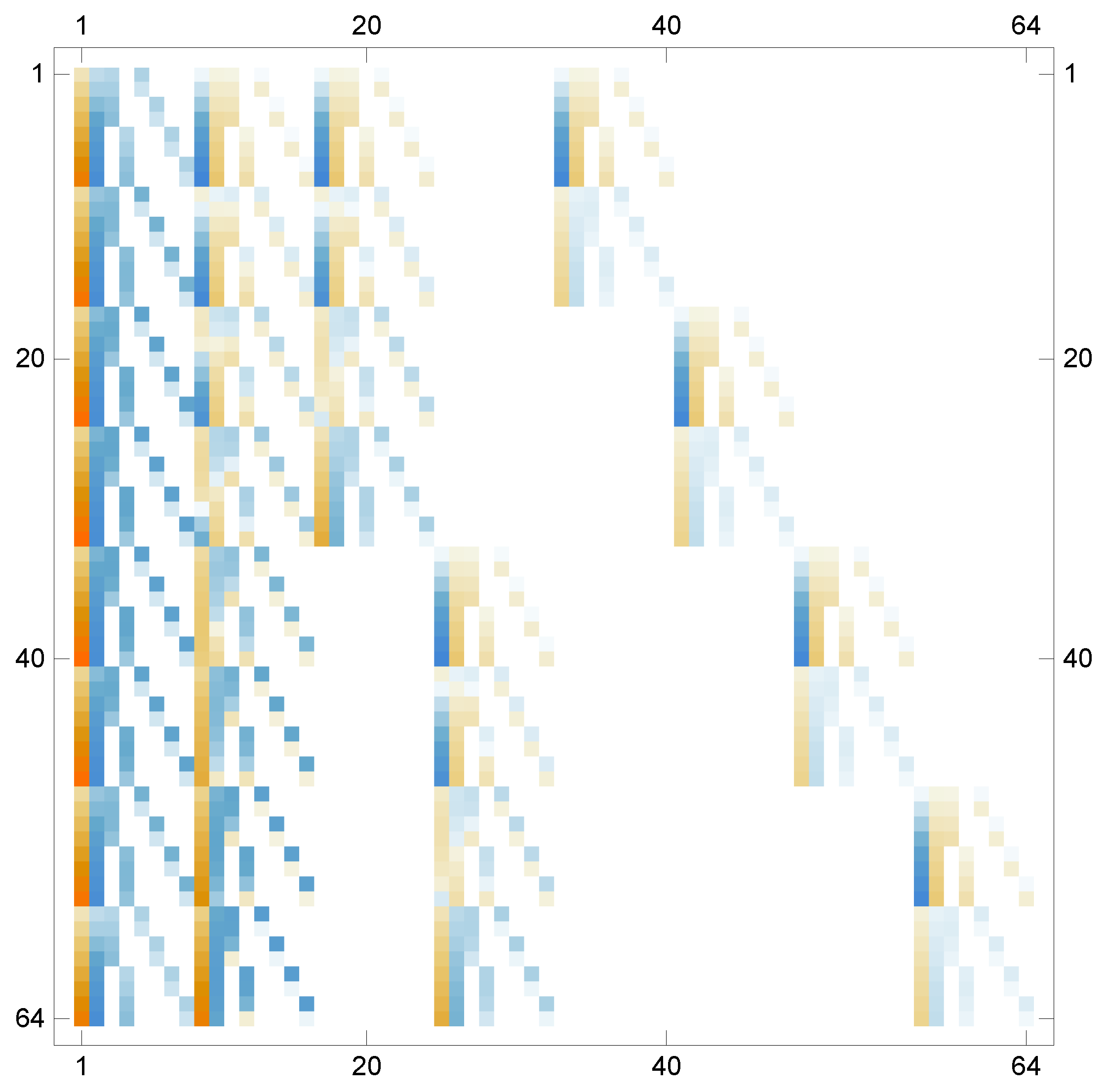
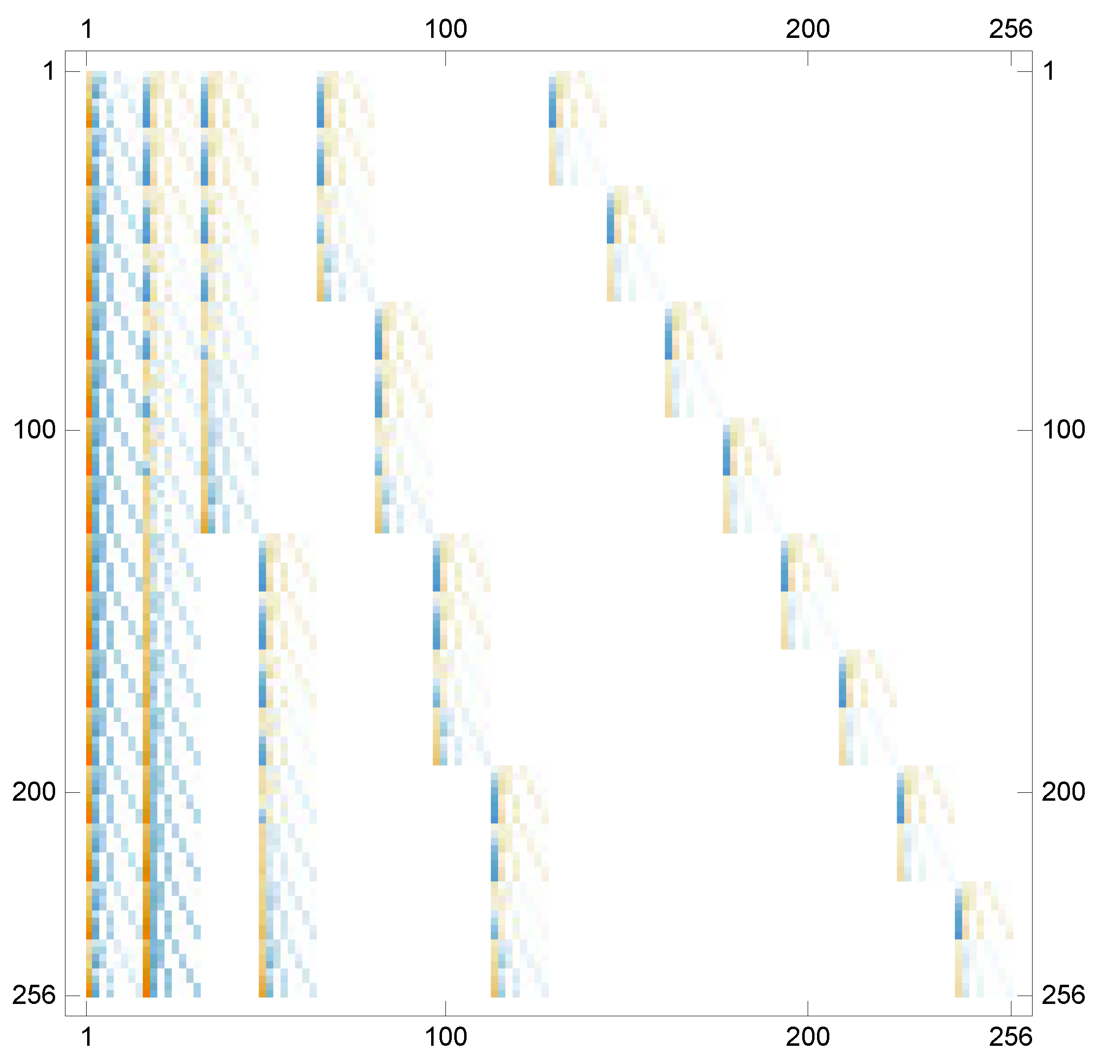
3. The New Numerical Scheme

Wavelets are basis set, very well localized functions, and known as a useful tool for solving various types of differential and integral equations. In particular, orthogonal wavelets are used extensively to approximate different types of fractional differential equations in the literature. To solve the proposed problem in Equations (1)–(3), we use wavelets based on Euler polynomials. We define the Euler polynomials $E_1\left(x\right),E_2\left(x\right)$ and the needed functions for our novel numerical algorithm as follows:

$$\begin{array}{ccc}\hfill E_1\left(x\right)& =& -\frac{1}{2}+x,E_2\left(x\right)=-x+x^2,\hfill \end{array}$$

(4)

$$\begin{array}{ccc}\hfill I_1^1& =& {\int }_0^x{E}_1\left(t\right)dt=-\frac{x}{2}+\frac{x^2}{2},\hfill \end{array}$$

(5)

$$\begin{array}{ccc}\hfill I_2^1& =& {\int }_0^x{E}_2\left(t\right)dt=-\frac{x^2}{2}+\frac{x^3}{3},\hfill \end{array}$$

(6)

$$\begin{array}{ccc}\hfill I_1^2& =& {\int }_0^x{I}_1^1\left(t\right)dt=-\frac{x^2}{4}+\frac{x^3}{6},\hfill \end{array}$$

(7)

$$\begin{array}{ccc}\hfill I_2^2& =& {\int }_0^x{I}_2^1\left(t\right)dt=-\frac{x^3}{6}+\frac{x^4}{12},\hfill \end{array}$$

(8)

$$\begin{array}{ccc}\hfill I_1^{\alpha }& =& {\int }_0^x\frac{E_1\left(\xi \right)}{{(x-\xi )}^{2-\alpha }}d\xi =\frac{x^{2-\alpha }(-3+\alpha +2x)}{2(-2+\alpha )(-3+\alpha )}\hfill \end{array}$$

(9)

$$\begin{array}{ccc}\hfill I_2^{\alpha }& =& {\int }_0^x\frac{E_2\left(\xi \right)}{{(x-\xi )}^{2-\alpha }}d\xi =-\frac{x^{3-\alpha }(-4+\alpha +2x)}{-6+11(\alpha -1)-6{(\alpha -1)}^2+{(\alpha -1)}^3}.\hfill \end{array}$$

(10)

Define $\Psi$ to be the set of all functions given in Equations (4)–(10). For any function $f\in \Psi$, we define the function $\psi \left(x\right)$ as follows

$$\begin{array}{ccc}\hfill \psi \left(x\right)& =& f\left(x\right),\mathit{on}[0,1],\hfill \\ & =& 0,\mathit{otherwise}.\hfill \end{array}$$

Now, assume that

$${\psi }_1=E_1,{\psi }_2=E_2,{\psi }_{1,1}=I_1^1,{\psi }_{2,1}=I_2^1,{\psi }_{1,2}=I_1^2,{\psi }_{2,2}=I_2^2,{\psi }_{1,\alpha }=I_1^{\alpha },{\psi }_{2,\alpha }=I_2^{\alpha },$$

we define the following set of functions (wavelets) depending on $j,k\in \mathbb{Z}$ as

$$\begin{array}{ccc}\hfill {\psi }_1(j,k,x)& =& {\psi }_1(2^{j}x-k),\hfill \\ \hfill {\psi }_2(j,k,x)& =& {\psi }_2(2^{j}x-k,),\hfill \\ \hfill \psi (j,k,x)& =& ({\psi }_1(j,k,x)+{\psi }_2(j,k,x)),\hfill \\ \hfill {\psi }^{1,1}(j,k,x)& =& {\psi }_{1,1}(2^{j}x-k),\hfill \\ \hfill {\psi }^{1,2}(j,k,x)& =& {\psi }_{1,2}(2^{j}x-k),\hfill \\ \hfill {\psi }^{2,1}(j,k,x)& =& {\psi }_{2,1}(2^{j}x-k),\hfill \\ \hfill {\psi }^{2,2}(j,k,x)& =& {\psi }_{2,2}(2^{j}x-k),\hfill \\ \hfill {\psi }^1(j,k,x)& =& ({\psi }^{1,1}(j,k,x)+{\psi }^{2,1}(j,k,x))/j,\hfill \\ \hfill {\psi }^2(j,k,x)& =& ({\psi }^{2,1}(j,k,x)+{\psi }^{2,2}(j,k,x))/j^2,\hfill \\ \hfill {\psi }^{1,\alpha }(j,k,x)& =& {\psi }_{1,\alpha }(2^{j}x-k),\hfill \\ \hfill {\psi }^{2,\alpha }(j,k,x)& =& {\psi }_{2,\alpha }(2^{j}x-k),\hfill \\ \hfill {\psi }^{\alpha }(j,k,x)& =& ({\psi }^{1,\alpha }(j,k,x)+{\psi }^{2,\alpha }(j,k,x))/j^{\alpha -2}.\hfill \end{array}$$

Recall that, see, e.g., [12], a function $f\in L_2\left(\mathbb{R}\right)$ can be expanded using the following series,

$$f\left(x\right)=\sum _{\ell =1}^2\sum _{j,k\in \mathbb{Z}}^{\infty }{d}^{\ell }(j,k){\psi }^{\ell }(j,k,x),$$

(11)

where,

$$d^{\ell }(j,k)=〈f,{\psi }^{\ell }(j,k,x)〉={\int }_{\mathbb{R}}f\left(x\right){\psi }^{\ell }(j,k,x)w\left(x\right)dx,$$

for which $〈·,·〉$ denotes the usual inner product over the space $L_2\left(\mathbb{R}\right)$ and w is a proper weight function. One may truncate Equation (11) by $f_{n,M}$ as

$$f_{n,M}=\sum _{\ell =1}^2\sum _{j=0}^n\sum _{k=0}^{M-1}{d}^{\ell }(j,k){\psi }^{\ell }(j,k,x).$$

(12)

In order to solve the proposed problem, we construct a vector ${\Psi }_f$ of length $M=2^{n+1},n\in \mathbb{N}$, such that

$${\Psi }_f=({\psi }_f,{\sigma }^{\rho }(1,0,x),\dots ,{\sigma }^{\rho }(2^j,k,x),\dots ,{\sigma }^{\rho }(2^n,2^{n-1},x)),j=0,1,2,\dots ,n;k=0,1,2,\dots ,2^{j-1},$$

(13)

where,

$$\left\{\begin{array}{cc}{\psi }_f=1,{\sigma }^{\rho }=\psi \hfill & iff=E_1,E_2,\rho =1,\hfill \\ {\psi }_f=x,{\sigma }^{\rho }={\psi }^1\hfill & iff=I_1^1,I_2^1,\rho =j,\hfill \\ {\psi }_f=x^2/2,{\sigma }^{\rho }={\psi }^2\hfill & iff=I_1^2,I_2^2,\rho =j^2,\hfill \\ {\psi }_f=I_1^{\alpha }\left(x\right),{\sigma }^{\rho }={\psi }^{\alpha }\hfill & iff=I_1^{\alpha },I_2^{\alpha },\rho =j^{\alpha -2}.\hfill \end{array}\right.$$

For example, for $n=2,\alpha =3/2$, we have the following:

• When ${\psi }_f=1,\rho =1$, we have

  $${\Psi }_f=\left\{\begin{array}{cc}\left(1,0,0,0,0,0,0,0\right)\hfill & x\ge 1orx<0\hfill \\ \left(1,x^2-\frac{1}{2},0,{(2x-1)}^2-\frac{1}{2},0,0,0,{(4x-3)}^2-\frac{1}{2}\right)\hfill & \frac{3}{4}\le x<1\hfill \\ \left(1,x^2-\frac{1}{2},0,{(2x-1)}^2-\frac{1}{2},0,0,{(4x-2)}^2-\frac{1}{2},0\right)\hfill & \frac{1}{2}\le x<\frac{3}{4}\hfill \\ \left(1,x^2-\frac{1}{2},4x^2-\frac{1}{2},0,0,{(4x-1)}^2-\frac{1}{2},0,0\right)\hfill & \frac{1}{4}\le x<\frac{1}{2}\hfill \\ \left(1,x^2-\frac{1}{2},4x^2-\frac{1}{2},0,16x^2-\frac{1}{2},0,0,0\right)\hfill & \mathrm{True}\hfill \end{array}\right.$$
• When ${\psi }_f=x,\rho =j$, we have

  $${\Psi }_f=\left\{\begin{array}{cc}\left(x,0,0,0,0,0,0,0\right)\hfill & x\ge 1orx<0\hfill \\ \left(x,\frac{1}{6}x\left(2x^2-3\right),0,\frac{1}{12}\left(16x^3-24x^2+6x+1\right),0,0,0,\frac{1}{12}{(4x-3)}^3+\frac{1}{8}(3-4x)\right)\hfill & \frac{3}{4}\le x<1\hfill \\ \left(x,\frac{1}{6}x\left(2x^2-3\right),0,\frac{1}{12}\left(16x^3-24x^2+6x+1\right),0,0,\frac{1}{12}\left(64x^3-96x^2+42x-5\right),0\right)\hfill & \frac{1}{2}\le x<\frac{3}{4}\hfill \\ \left(x,\frac{1}{6}x\left(2x^2-3\right),\frac{1}{6}x\left(8x^2-3\right),0,0,\frac{16x^3}{3}-4x^2+\frac{x}{2}+\frac{1}{24},0,0\right)\hfill & \frac{1}{4}\le x<\frac{1}{2}\hfill \\ \left(x,\frac{1}{6}x\left(2x^2-3\right),\frac{1}{6}x\left(8x^2-3\right),0,\frac{1}{6}x\left(32x^2-3\right),0,0,0\right)\hfill & \mathrm{True}\hfill \end{array}\right.$$
• When ${\psi }_f=x^2/2,\rho =j^2$, we have

  $${\Psi }_f=\left\{\begin{array}{cc}\left(\frac{x^2}{2},0,0,0,0,0,0,0\right)\hfill & x\ge 1orx<0\hfill \\ \left(\frac{x^2}{2},\frac{1}{12}{x}^2\left(x^2-3\right),0,\frac{1}{24}{(1-2x)}^2\left(2x^2-2x-1\right),0,0,0,\frac{1}{96}{(3-4x)}^2\left(8x^2-12x+3\right)\right)\hfill & \frac{3}{4}\le x<1\hfill \\ \left(\frac{x^2}{2},\frac{1}{12}{x}^2\left(x^2-3\right),0,\frac{1}{24}{(1-2x)}^2\left(2x^2-2x-1\right),0,0,\frac{1}{48}{(1-2x)}^2\left(16x^2-16x+1\right),0\right)\hfill & \frac{1}{2}\le x<\frac{3}{4}\hfill \\ \left(\frac{x^2}{2},\frac{1}{12}{x}^2\left(x^2-3\right),\frac{1}{12}{x}^2\left(4x^2-3\right),0,0,\frac{1}{96}{(1-4x)}^2\left(8x^2-4x-1\right),0,0\right)\hfill & \frac{1}{4}\le x<\frac{1}{2}\hfill \\ \left(\frac{x^2}{2},\frac{1}{12}{x}^2\left(x^2-3\right),\frac{1}{12}{x}^2\left(4x^2-3\right),0,\frac{4x^4}{3}-\frac{x^2}{4},0,0,0\right)\hfill & \mathrm{True}\hfill \end{array}\right.$$
• When ${\psi }_f=I_1^{\alpha },\rho =j^{\alpha -2}$, we have

  $${\Psi }_f=\left\{\begin{array}{cc}\left(2\sqrt{x},0,0,0,0,0,0,0\right)\hfill & x\ge 1orx<0\hfill \\ \left(2\sqrt{x},x^2-\frac{1}{2},0,\frac{8x^2-8x+1}{\sqrt{2}},0,0,0,32x^2-48x+17\right)\hfill & \frac{3}{4}\le x<1\hfill \\ \left(2\sqrt{x},x^2-\frac{1}{2},0,\frac{8x^2-8x+1}{\sqrt{2}},0,0,32x^2-32x+7,0\right)\hfill & \frac{1}{2}\le x<\frac{3}{4}\hfill \\ \left(2\sqrt{x},x^2-\frac{1}{2},\frac{8x^2-1}{\sqrt{2}},0,0,32x^2-16x+1,0,0\right)\hfill & \frac{1}{4}\le x<\frac{1}{2}\hfill \\ \left(2\sqrt{x},x^2-\frac{1}{2},\frac{8x^2-1}{\sqrt{2}},0,32x^2-1,0,0,0\right)\hfill & \mathrm{True}\hfill \end{array}\right.$$

Now, define the solution of the proposed system given in Equations (1)–(3) in the form of a matrix system by the following equation,

$$\begin{array}{c}{u}_{xxtt}\approx {\Psi }_E^T\left(x\right)·U·{\Psi }_E\left(t\right),\end{array}$$

(14)

where U is a matrix of order $M\times M$ that should be determined using some collocation points, ${\Psi }_E^T$ is the transpose of the vector ${\Psi }_E$ and E denotes the set of both functions $E_1$ and $E_1$ that are defined earlier.

Integrating Equation (14) step by step two times with respect to t yields:

$$\begin{array}{ccc}\hfill u_{xxt}(x,t)& \approx & {\Psi }_E^T\left(x\right)·U·{\Psi }_{I^1}\left(t\right)+F_1^{{}^{″}}\left(x\right),\hfill \\ \hfill u_{xx}(x,t)& \approx & {\Psi }_E^T\left(x\right)·U·{\Psi }_{I^2}\left(t\right)+t{F}_1^{{}^{″}}\left(x\right)+F_2^{{}^{″}}\left(x\right),\hfill \end{array}$$

Now, integrating Equation (14) step by step two times for x, reveals the following:

$$\begin{array}{ccc}\hfill u_x(x,t)& \approx & {\Psi }_{I^1}^T\left(x\right)·U·{\Psi }_{I^2}\left(t\right)+t(F_1^{{}^{\prime }}\left(x\right)-F_1^{{}^{\prime }}\left(0\right))+F_2^{{}^{\prime }}\left(x\right)-F_2^{{}^{\prime }}\left(0\right)+F_3\left(t\right),\hfill \\ \hfill u(x,t)& \approx & {\Psi }_{I^2}^T\left(x\right)·U·{\Psi }_{I^2}\left(t\right)+t(F_1\left(x\right)-F_1\left(0\right)-x{F}_1^{{}^{\prime }}\left(0\right))+F_2\left(x\right)-F_2\left(0\right)-x{F}_2^{{}^{\prime }}\left(0\right)+x{F}_3\left(t\right)+F_4\left(t\right),\hfill \end{array}$$

where

$$I^1=\left\{I_1^1,I_2^1\right\},I^2=\left\{I_1^2,I_2^2\right\},$$

and $F_1\left(x\right),F_2\left(x\right),F_3\left(t\right),F_4\left(t\right)$ are arbitrary functions that can be determined using the initial and boundary conditions given in Equation (3).

Hence, we have

$$\begin{array}{ccc}\hfill u(x,t)& \approx & {\Psi }_{I^2}^T\left(x\right)·U·{\Psi }_{I^2}\left(t\right)+t(f_1\left(x\right)-(x{F}_3^{{}^{\prime }}\left(0\right)+F_4^{{}^{\prime }}\left(0\right)))+f_0\left(x\right)-x{F}_3\left(0\right)-F_4\left(0\right)+x{F}_3\left(t\right)+g_0\left(t\right),\hfill \\ \hfill u_t(x,t)& \approx & {\Psi }_{I^2}^T\left(x\right)·U·{\Psi }_{I^1}\left(t\right)+f_1\left(x\right)-x{F}_3^{{}^{\prime }}\left(0\right)-F_4{}^{\prime }\left(0\right)+x{F}_3^{{}^{\prime }}\left(t\right)+g_0^{{}^{\prime }}\left(t\right),\hfill \\ \hfill u_{xx}(x,t)& \approx & {\Psi }_E^T\left(x\right)·U·{\Psi }_{I^2}\left(t\right)+t{f}_1^{{}^{″}}\left(x\right)+f_0^{{}^{″}}\left(x\right),\hfill \\ \hfill u_{tt}(x,t)& \approx & {\Psi }_{I^2}^T\left(x\right)·U·{\Psi }_E\left(t\right)+x{F}_3^{{}^{″}}\left(t\right)+g_0^{{}^{″}}\left(t\right),\hfill \\ \hfill {\mathcal{D}}_c^{\alpha }u(x,t)& \approx & {\displaystyle \frac{1}{\Gamma (2-\alpha )}}\left(-x{\Psi }_{I^2}^T\left(x\right)·U·{\Psi }_{I^{\alpha }}\left(t\right)+{\Psi }_{I^2}^T\left(x\right)·U·{\Psi }_{I^{\alpha }}\left(t\right)+F_5\left(t\right)+x{F}_6\left(t\right)\right),\hfill \end{array}$$

where

$$I^{\alpha }=\left\{I_1^{\alpha },I_2^{\alpha }\right\}.$$

Here, we define the functions $F_i$ as follows

$$\begin{array}{ccc}\hfill F_4\left(t\right)& =& g_0\left(t\right),\hfill \\ \hfill F_3\left(t\right)& =& g_1\left(t\right)-g_0\left(t\right)-{\Psi }_{I^2}^T\left(t\right)·U·{\Psi }_{I^2}\left(t\right)+t{c}_1+c_2,\hfill \\ \hfill F_5\left(t\right)& =& {\int }_0^t\frac{g_0^{{}^{″}}\left(\tau \right)}{{(t-\tau )}^{2-\alpha }}d\tau ,\hfill \\ \hfill F_6\left(t\right)& =& {\int }_0^t\frac{g_1^{{}^{″}}\left(\tau \right)-g_0^{{}^{″}}\left(\tau \right)}{{(t-\tau )}^{2-\alpha }}d\tau ,\hfill \\ \hfill c_0& =& g_1\left(0\right)-2g_0\left(0\right)+f_0\left(1\right),\hfill \\ \hfill c_1& =& -f_1\left(1\right)+c_0/2+g_0\left(0\right),\hfill \\ \hfill c_2& =& -f_0\left(1\right)+c_0/2+g_0\left(0\right).\hfill \end{array}$$

Now, we have all functions needed for the numerical simulation. Let us define $M=2^{1+n},n=1,2,..$ as a collocation points and

$$\Delta x=1/M,s_0=0,s_i=s_{i-1}+\Delta x,i=1,2,..,M;x_i=t_i=\frac{1}{2}(s_{i-1}+s_i),i=1,2,\dots ,M.$$

Then, we substitute the above equations into the propose system and calculate Equation (1) for each pair of the collocation points as follows

$${\mathcal{D}}_c^{\alpha }u(x_i,t_j)+\mu u_t(x_i,t_j)-u_{xx}(x_i,t_j)=Q(x_i,t_j),i,j=1,2,\dots ,M.$$

(15)

Therefore,

$$\begin{array}{ccc}& & {\displaystyle \frac{1}{\Gamma (2-\alpha )}}\left(-x_i{\Psi }_{I^2}^T\left(x_i\right)·U·{\Psi }_{I^{\alpha }}\left(t_j\right)+{\Psi }_{I^2}^T\left(x_i\right)·U·{\Psi }_{I^{\alpha }}\left(t_j\right)+F_5\left(t_j\right)+x_i{F}_6\left(t_j\right)\right)+\hfill \end{array}$$

(16)

$$\begin{array}{ccc}& & \mu \left({\Psi }_{I^2}^T\left(x_i\right)·U·{\Psi }_{I^1}\left(t_j\right)+f_1\left(x_i\right)-x_i{F}_3^{{}^{\prime }}\left(0\right)-F_4{}^{\prime }\left(0\right)+x_i{F}_3^{{}^{\prime }}\left(t_j\right)+g_0^{{}^{\prime }}\left(t_i\right)\right)-\hfill \end{array}$$

(17)

$$\begin{array}{ccc}& & \left({\Psi }_E^T\left(x\right)·U·{\Psi }_{I^2}\left(t\right)+t{f}_1^{{}^{″}}\left(x\right)+f_0^{{}^{″}}\left(x\right)\right)=Q(x_i,t_j)\hfill \end{array}$$

(18)

Note that Equations (16)–(18) generates an $M\times M$ system of algebraic equations in order to produce our matrix U.

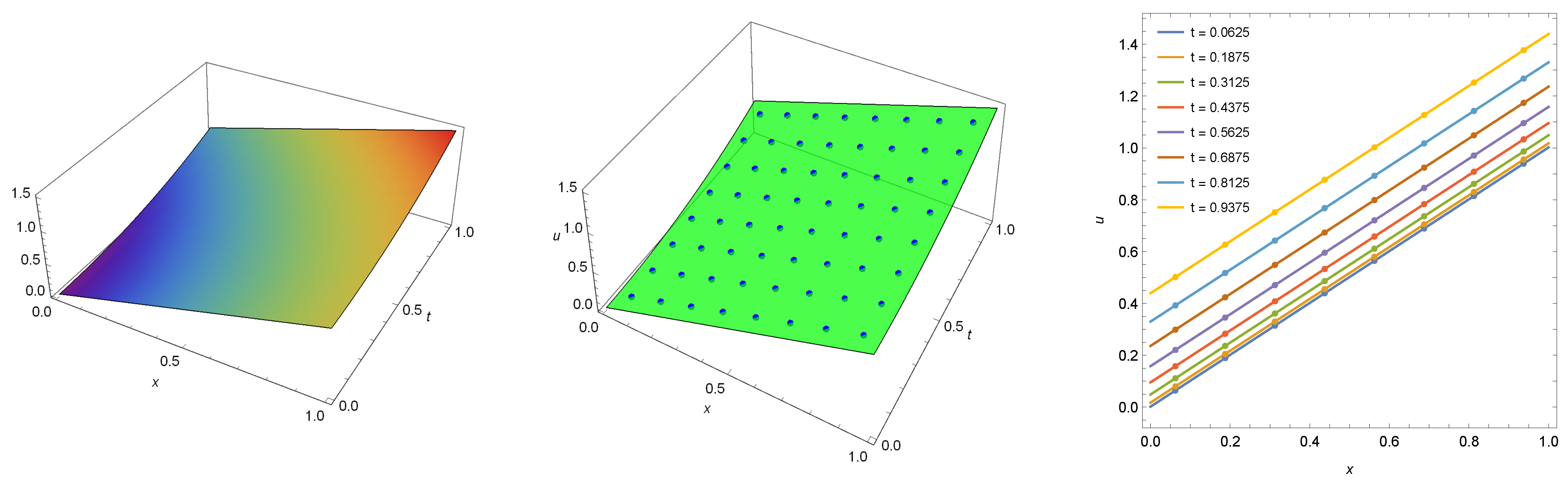
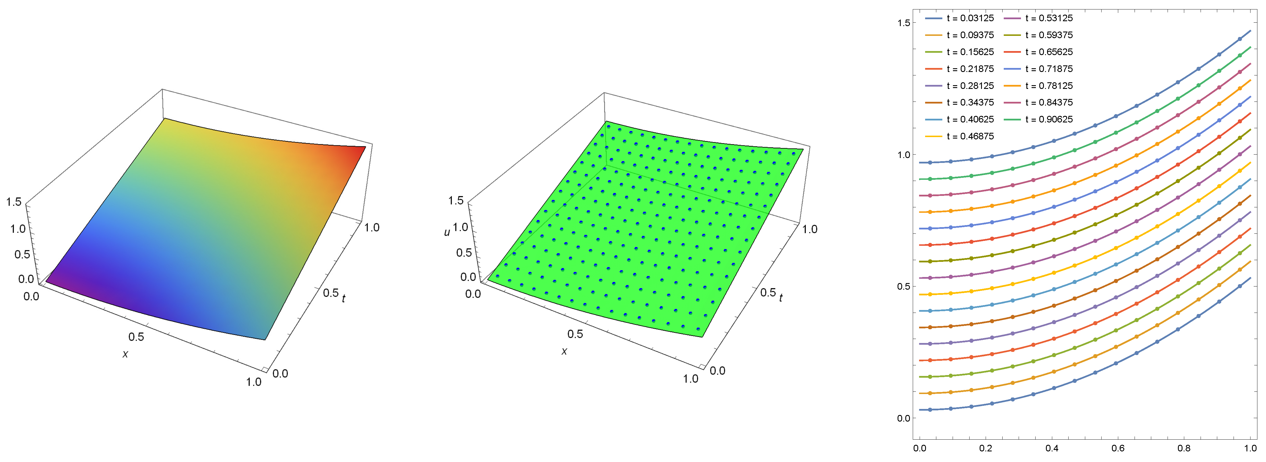
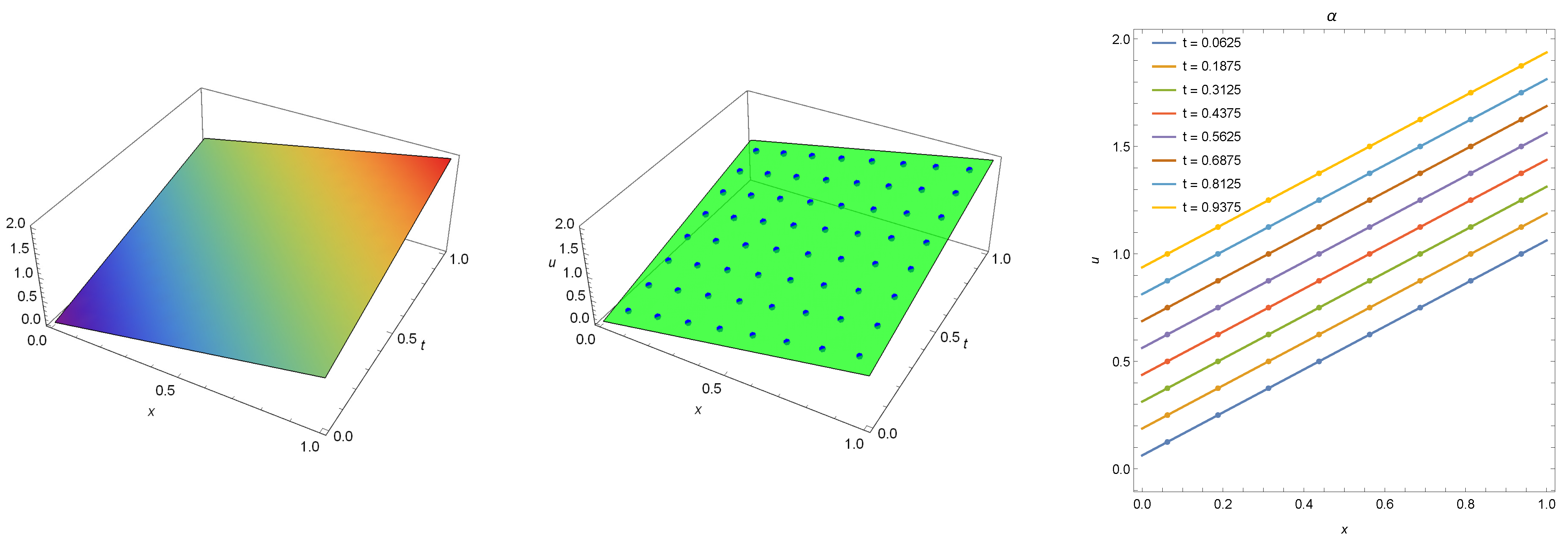
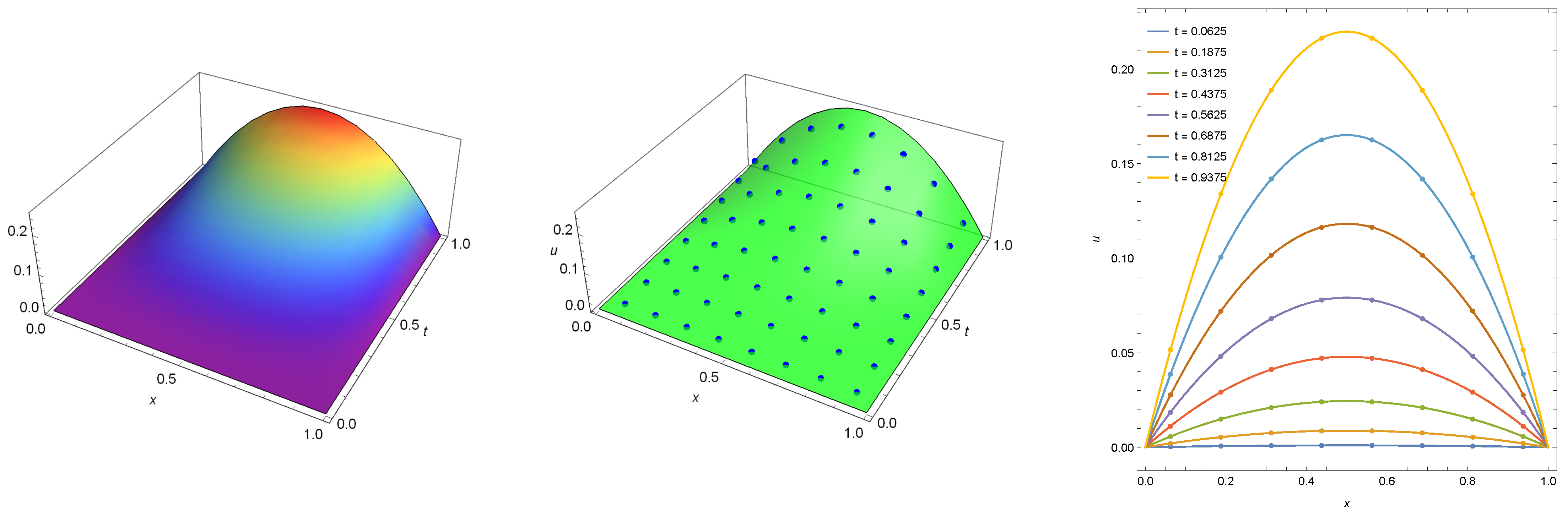
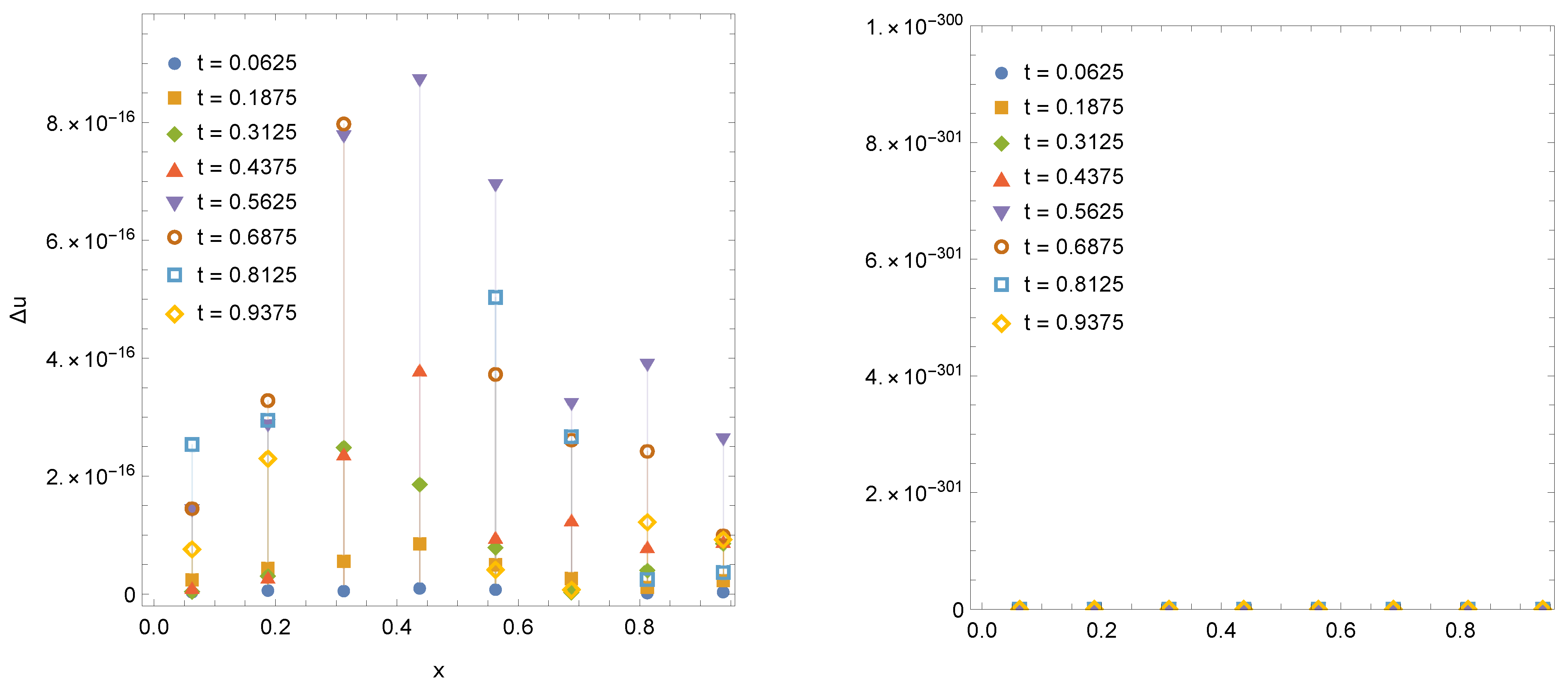
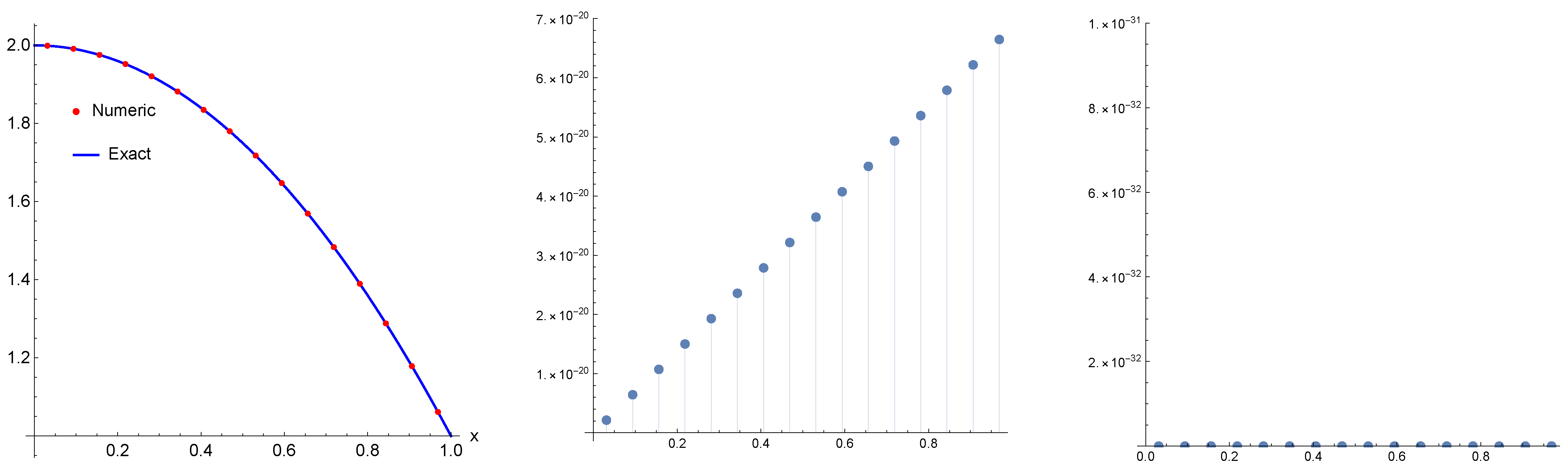
4. Numerical Performance

In this section, we present some examples of the problem proposed in Equations (1)–(3). The numerical solution demonstrated here achieved a zero absolute error and that was independent from the number of collocation points, damping parameter $\mu$ and fractional value $\alpha$. We noticed that there is a numerical phenomenon behind the error cancellation in this method.

The generated system of algebraic equations given in Equation (15) is not so simple and it is also a matrix; however, for all examples that we consider, the numerical solution is not different from the exact solution in all collocation points and that makes this technique a special and powerful tool capable of achieving such an excellent order of accuracy.

Example 1.

Consider the equation

$${\mathcal{D}}_c^{\alpha }u(x,t)+\mu u_t(x,t)-u_{xx}(x,t)=Q(x,t),$$

(19)

where,

$$Q(x,t)=\frac{1}{\Gamma (2-\alpha )}{\int }_0^t\frac{u_{\tau \tau }(x,\tau )}{{(t-\tau )}^{2-\alpha }}d\tau ,1<\alpha \le 2,$$

with the following initial and boundary condition given as

$$u(x,0)=x,u_t(x,0)=0,u(0,t)=(2-\alpha )t^2,u(1,t)=1+(2-\alpha )t^2.$$

(20)

The exact solution for this formulation is

$$u_e(x,t)=x+(2-\alpha )t^2.$$

Applying our algorithm, Figure 1 presents the exact solution (left) and exact solution with numerical solution (middle and right) computed at $M=8,\mu =1,\alpha =3/2$. The maximum absolute error for the numerical solution is calculated by Mathematica as zero and so it is less than the minimal machine number $2.22507\times {10}^{-308}$, which means

$$max|u(x_i,t_j)-u_e(x_i,t_j)|<2.22507\times {10}^{-308},i,j=1,2,\dots ,M.$$

Figure 2 shows the visual representation of the values of elements in the matrix generated during solving the related system of algebraic equations for this example.

Example 2.

Consider the equation

$${\mathcal{D}}_c^{\alpha }u(x,t)+\mu u_t(x,t)-u_{xx}(x,t)=0.$$

(21)

with the following initial and boundary condition given as

$$u(x,0)=\frac{x^2}{2},u_t(x,0)=\frac{1}{\mu },u(0,t)=\frac{t}{\mu },u(1,t)=\frac{1}{2}+\frac{t}{\mu }.$$

(22)

The exact solution for this formulation is

$$u_e(x,t)=\frac{x^2}{2}+\frac{t}{\mu }.$$

In Figure 3, we show the exact solution (left) and exact solution with numerical solution (middle and right) computed at $M=16,\mu =1,\alpha =19/10$. Again, the maximum absolute error for the numerical solution is recognized by Mathematica as zero. Thus, it is less than the minimal machine number $2.22507\times {10}^{-308}$.

Figure 4 shows the visual representation of the values of elements in the matrix generated during solving the related system of algebraic equations.

Example 3.

The numerical phenomenon of the error cancellation also occurs for the wave equation. In this case, we have $\alpha =2$, and so Equation (1) turns to the common form of the wave equation given by

$$u_{tt}(x,t)+\mu u_t(x,t)-u_{xx}(x,t)=Q(x,t),$$

(23)

where,

$$Q(x,t)=\mu .$$

The initial and boundary conditions are given as

$$u(x,0)=x,u_t(x,0)=1,u(0,t)=t,u(1,t)=1+t.$$

(24)

The exact solution of this problem is $u_e(x,t)=x+t$. In Figure 5, we present the exact solution (left) and exact solution with numerical solution (middle and right) computed at $M=8,\mu =1,\alpha =2$. The maximum absolute error for the numerical solution is zero for this case as well.

Example 4.

The numerical phenomenon of the error cancellation also occurs for the wave equation. In this case, we choose $\alpha =3/2$, and so Equation (1) turns to the common form of the wave equation given by

$${\mathcal{D}}_c^{\alpha }u(x,t)+\mu u_t(x,t)-u_{xx}(x,t)=Q(x,t),$$

(25)

where,

$$Q(x,t)=\mu x.$$

The initial and boundary conditions are given as

$$u(x,0)=0,u_t(x,0)=x,u(0,t)=0,u(1,t)=t.$$

(26)

The exact solution of this problem is $u_e(x,t)=xt$. In Figure 6, we present the exact solution (left) and exact solution with numerical solution (middle and right) computed at $M=8,\mu =1,\alpha =2$. The maximal absolute error for the numerical solution is zero. This result does not depend on the number of collocation points, nor the fractional parameters α and μ.

Example 5.

Let us consider another example by involving the fractional parameter α in the function Q as follows

$${\mathcal{D}}_c^{\alpha }u(x,t)+\mu u_t(x,t)-u_{xx}(x,t)=\frac{2x(1-x)t^{2-\alpha }}{(2-\alpha )\Gamma (2-\alpha )}+2tx(1-x)+2t^2.$$

(27)

The initial and boundary conditions are given as

$$u(x,0)=0,u_t(x,0)=0,u(0,t)=0,u(1,t)=0.$$

(28)

This example has been considered and discussed for $\mu =1$ by many authors, see, e.g., [11,13,14]. The exact solution for this case has the following form $u_e=t^{2}x(1-x)$. Using our technique, we are able to solve it with a proper setting of precision of the numerical technique. For instance, in Figure 7, we provide the exact solution and numerical solution (points) computed with machine precision of $1.11022\times {10}^{-16}$ ( shown in Figure 8, left). Increasing precision up to ${10}^{-30}$, we get the numerical solution with zero absolute error (as it shown in Figure 8, right).

5. Numerical Technique for Nonlinear Fredholm and Volterra Integral Equation

Let us now consider the following form of Volterra integral equation of the second kind

$$u\left(x\right)=g\left(x\right)+{\int }_0^{x}K(x,t,u\left(t\right))dt,0\le x\le 1,$$

(29)

where g and K (the kernel) are known functions. It is well known that Equation (29) has a unique solution under following conditions [15]:

(1)

$g\left(x\right)$ is continues and bounded on $0\le x\le 1$;

(2)

The kernel $K(x,t,u)$ is bounded and uniformly continuous in both x and t, for all finite u where $0\le t\le x\le 1$;

(3)

The kernel $K(x,t,u)$ satisfies the uniform Lipschitz condition

$$|K(x,t,u_1)-K(x,t,u_2)|\le L|u_1-u_2|,$$

(30)

for all finite $u_{1,2}$ and $0\le t\le x\le 1$.

To solve Equation (29), we use Euler wavelets in the form of vector ${\Psi }_E$ that we defined earlier. Then, we proposed that the numerical solution has the following setting:

$$u\left(x\right)=A·{\Psi }_E\left(x\right),$$

(31)

where the vector $A=(a_1,a_2,...,a_M)$ can be computed using the collocation technique such that

$$M=2^{1+n},n=1,2,...,$$

and ${\Psi }_E\left(x\right)$ is defined considering $\rho \left(j\right)=2$.

To do this, we first transform the integral in Equation (29) by substituting

$$t=\frac{x}{2}(s+1),-1\le s\le 1.$$

Then, this integral turns to the fixed limit integral, and so it can be approximated by a finite sum using the Gauss quadrature rule as follows:

$$\begin{array}{ccc}\hfill {\int }_0^{x}K(x,t,u\left(t\right))dt& =& \frac{x}{2}{\int }_{-1}^{1}K(x,x(s+1)/2,u(x(s+1)/2))ds\hfill \end{array}$$

(32)

$$\begin{array}{ccc}\hfill & =& \frac{x}{2}\sum _{i=1}^{2M}{w}_{i}K(x,x(s_i+1)/2,u(x(s_i+1)/2))+\Delta ,\hfill \end{array}$$

(33)

where $w_i$ are weights, $s_i$ are points of the Gauss quadrature rule defined on $(-1,1)$, and $\Delta$ is the error of approximation. Substituted Equations (31) and (32) in Equation (29) and using the assumed collocation points, we get a system of algebraic equations:

$$A·{\Psi }_E\left(x_j\right)=g\left(x_j\right)+\frac{x_j}{2}\sum _{i=1}^{2M}{w}_{i}K(x_j,x_j(s_i+1)/2,A·{\Psi }_E(x_j(s_i+1)/2)),$$

(34)

for $j=1,2,...,M$ and $\Delta =0$.

The system of nonlinear algebraic equations given in Equation (34) can be solved by using several method. In this work, we use Newton’s iterative technique.

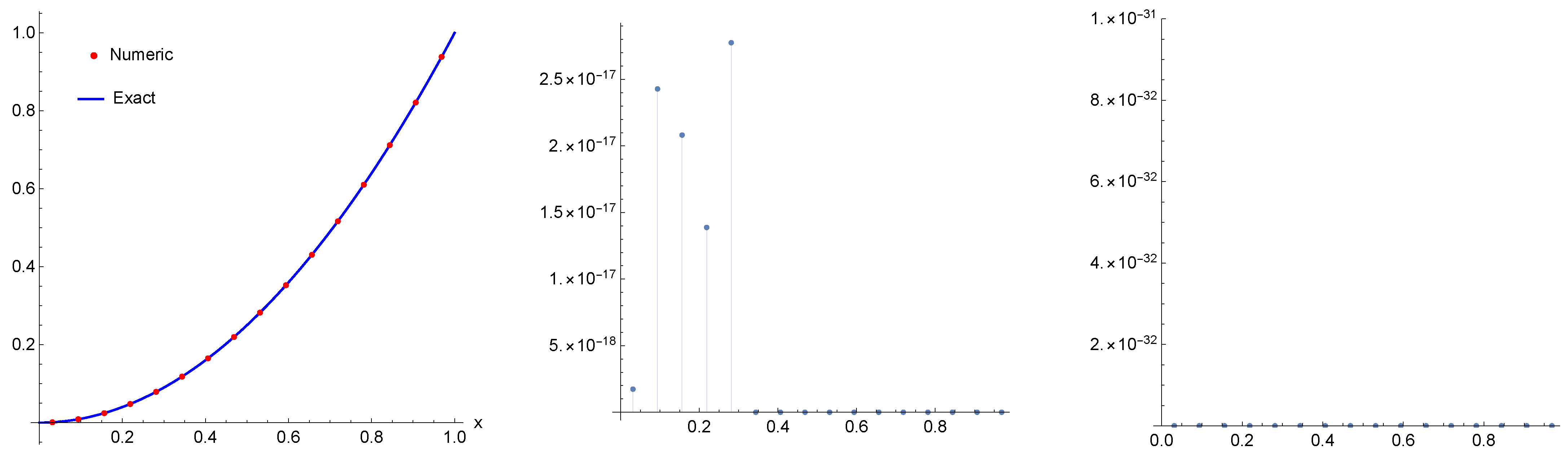
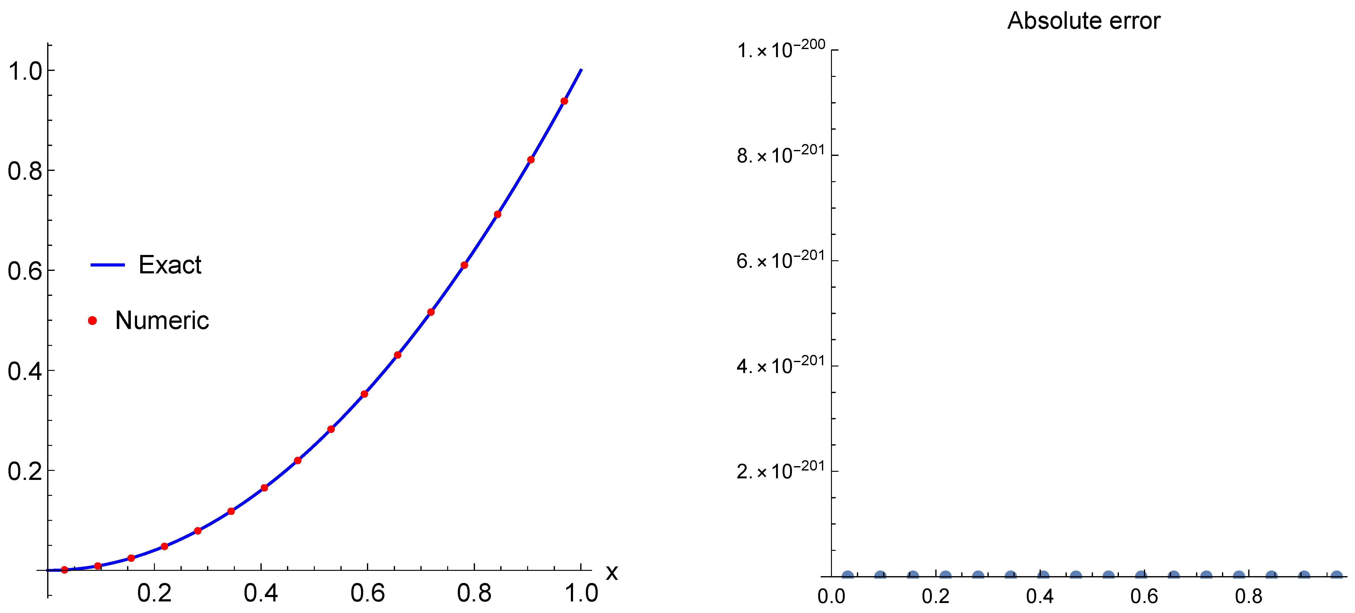
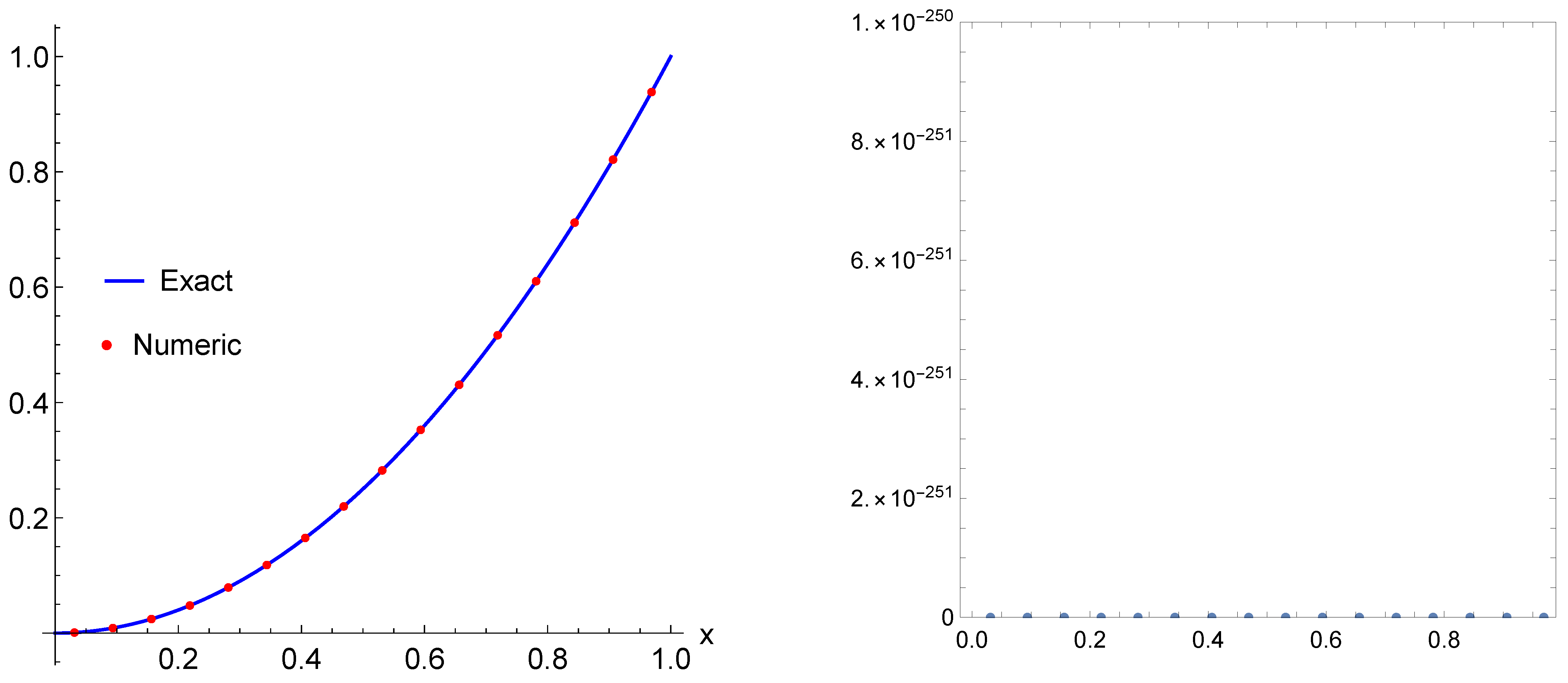
6. Numerical Examples

The parameters of the Gauss quadrature rule are not exact; however, it can be calculated with high precision of ${10}^{-60}$, it is possible to solve the system in Equation (34) with absolute error of $0\times {10}^{-31}$. We can consider this solution as a numerical solution with zero absolute error without future estimation. For the examples in this section, the numerical solution has absolute error as of $0\times {10}^{-31}$. Furthermore, we consider some intermediate results computed with machine precision as of $1.11022\times {10}^{-16}$.

Example 6.

This example has been discussed by many authors, see for example [16,17,18]:

$$u\left(x\right)=\frac{x^2}{2}(1+cos{x}^2)+{\int }_0^{x}t{x}^{2}sin\left(u\left(t\right)\right)dt$$

(35)

The exact solution of this equation is given by $u=x^2$. Using an iterative multistep kernel method [16] it is possible to get the numerical solution of Equation (35) with absolute error of $7.8974\times {10}^{-10}$, and using the method proposed in [17], the best result has absolute error of ${10}^{-6}$. Using our method, we get numerical solution with maximum absolute error of $2.77556\times {10}^{-17}$ computed with the machine precision (Figure 9, left and middle) and of 0 ×${10}^{-31}$ computed with double precision and with precision of ${10}^{-60}$ for the Gauss quadrature rule parameters $w_i,s_i$ (Figure 9, right). Note that, we have used $\rho \left(j\right)=2$ for this case.

Example 7.

Now, we consider the following nonlinear Fredholm integral Equation [19,20]:

$$u\left(x\right)=-x^2-\frac{x}{3}(2\sqrt{2}-1)+2+{\int }_0^{1}xt\sqrt{u\left(t\right)}dt$$

(36)

The exact solution for this problem is $u\left(x\right)=2-x^2$. This problem can be solved by the Haar wavelets method as in [19,20] with absolute error of $3.1\times {10}^{-5}$, $4.2\times {10}^{-6}$, respectively, where they used 128 collocation points to get into these bounds. With our method, with only 16 collocation points, we have achieved a numerical solution with absolute error of $6.64685\times {10}^{-20}$ computed using the machine precision, and as of 0 ×${10}^{-31}$ computed using a double precision as shown in Figure 10.

Example 8.

We consider now the following nonlinear Volterra integral equation based on two parameters such that

$$u\left(x\right)=x^2-\frac{x^{5+\beta +\gamma }}{5+\gamma }+{\int }_0^x{x}^{\beta }{t}^{\gamma }{u}^2\left(t\right)dt.$$

(37)

The exact solution of this equation is $u=x^2$. Numerical experiments with different $\beta ,\gamma$ shown that for any integer $\beta ,\gamma =0,1,2,\dots ,27$ the numerical solution has zero absolute error for all collocation points and for $n=3$. For integer $\gamma =0,1,2,\dots ,27$ and for some $1\le \beta \le 27$ including π and e the numerical solution has zero absolute error. For non integer $\beta ,\gamma >1$ there is absolute error that varies from zero up to ${10}^{-15}$. However, we cannot check every $\beta ,\gamma$ due to numerical limitations. The graphs of the exact, numerical and error results are depicted in Figure 11.

Example 9.

Finally, we consider the generalized form of Equation (35) based on two parameters as

$$u\left(x\right)=x^2-\frac{{}_1{F}_2(\frac{3+\gamma }{4};\frac{3}{2},\frac{7+\gamma }{4};-\frac{x^4}{4})}{3+\gamma }{x}^{3+\beta +\gamma }+{\int }_0^x{x}^{\beta }{t}^{\gamma }sin\left(u\left(t\right)\right)dt,$$

(38)

where ${}_1{F}_2(a;b;z)$ is the generalized hyper-geometric function. The exact solution of this formulation is $u=x^2$. Note that, Equation (35) is a special case of Equation (38) when $\beta =2,\gamma =1$. The numerical experiments for any integer $\beta ,\gamma =0,1,2,\dots ,80$ demonstrate a numerical solution with zero absolute error up to $\beta =30,\gamma =30$, and then maximum absolute error increases from $9\times {10}^{-50}$ for $\beta =31,\gamma =31$ to $1.01\times {10}^{-28}$ for $\beta =80,\gamma =80$. For any integer $\gamma =0,1,2,\dots ,30$ and real $0\le \beta \le 30$, the numerical solution has zero absolute error for all tested points including π and e. We present the exact, numerical and error results in Figure 12.

7. Conclusions

In this work, a novel numerical method based on a proper wavelet systems generated via Euler functions is proposed. The collocation algorithm based on Euler wavelets has been applied to the time-fractional diffusion wave and nonlinear Fredholm and Volterra integral equations. We used some truncated representations based on Euler wavelets to convert the proposed equations to a system of algebraic equations based on specific discretization. The reduced system was converted to a matrix form and simulated using Mathematica software.

We numerically solved a series of examples related to the proposed equations, where the numerical results achieved an exceptional absolute error among other numerical schemes in the literature. We provided some graphical illustrations to show the efficiency of the method.

References

1. Ghanbari, B.; Atangana, A. A new application of fractional Atangana–Baleanu derivatives: Designing ABC-fractional masks in image processing. Phys. A Stat. Mech. Appl. 2020, 542, 123516. [Google Scholar] [CrossRef]
2. Mohammad, M.; Trounev, A.; Cattani, C. An efficient method based on framelets for solving fractional Volterra integral equations. Entropy 2020, 22, 824. [Google Scholar] [CrossRef] [PubMed]
3. Mohammad, M.; Trounev, A. On the dynamical modeling of COVID-19 involving Atangana-Baleanu fractional derivative and based on Daubechies framelet simulations. Chaos Solitons Fractals 2020, 140, 110171. [Google Scholar] [CrossRef] [PubMed]
4. Mohammad, M.; Trounev, A. Fractional nonlinear Volterra–Fredholm integral equations involving Atangana–Baleanu fractional derivative: Framelet applications. Adv. Differ. Equ. 2020, 618, 1–15. [Google Scholar] [CrossRef]
5. Mohammad, M.; Trounev, A.; Cattani, C. The dynamics of COVID-19 in the UAE based on fractional derivative modeling using Riesz wavelets simulation. Adv. Differ. Equ. 2021, 2021, 1–14. [Google Scholar] [CrossRef] [PubMed]
6. Alshbool, H.M.; Isik, O.; Hashim, I. Fractional Bernstein series solution of fractional diffusion equations with error estimate. Axioms 2021, 10, 6. [Google Scholar] [CrossRef]
7. Mohammad, M. Biorthogonal-Wavelet-Based Method for Numerical Solution of Volterra Integral Equations. Entropy 2019, 21, 1098. [Google Scholar] [CrossRef] [Green Version]
8. Ferrari, A.; Gadella, M.; Lara, L.P.; Santillan, E. Approximate solutions of one dimensional systems with fractional calculus. Int. J. Mod. Phys. C 2020, 31, 2050092. [Google Scholar] [CrossRef]
9. Fernando, O.R.; Oscar, R.O. Transition from the Wave Equation to Either the Heat or the Transport Equations through Fractional Differential Expressions. Symmetry 2018, 10, 524. [Google Scholar] [CrossRef] [Green Version]
10. Rajagopal, N.; Balaji, S.; Seethalakshmi, R.; Balaji, V.S. A new numerical method for fractional order volterra integro-differential equations. Ain Shams Eng. J. 2020, 11, 171–177. [Google Scholar] [CrossRef]
11. Zhou, F.; Xu, X. Numerical solution of time-fractional diffusion-wave equations via chebyshev wavelets collocation method. Adv. Math. Phys. 2017, 2017, 1–17. [Google Scholar] [CrossRef] [Green Version]
12. Mohammad, M.; Lin, E.B. Gibbs phenomenon in tight framelet expansions. Commun. Nonlinear Sci. Numer. Simul. 2018, 55, 84–92. [Google Scholar] [CrossRef]
13. Heydari, M.H.; Hooshmandasl, M.R.; Maalek Ghaini, F.M.; Cattani, C. Wavelets method for the time fractional diffusion-wave equation. Phys. Lett. A 2015, 379, 71–76. [Google Scholar]
14. Chen, J.; Liu, F.; Anh, V.; Shen, S.; Liu, Q.; Liao, C. The analytical solution and numerical solution of the fractional diffusion-wave equation with damping. Appl. Math. Comput. 2012, 219, 1737–1748. [Google Scholar] [CrossRef] [Green Version]
15. Tricomi, F.G. Integral equations. In Pure and Applied Mathematics; Dover Publications: New York, NY, USA, 1957; Volume 5, p. 238. [Google Scholar]
16. Heydari, M.; Shivanian, E.; Azarnavid, B.; Abbasbandy, S. An iterative multistep kernel based method for nonlinear volterra integral and integro-differential equations of fractional order. J. Comput. Appl. Math. 2019, 361, 97–112. [Google Scholar] [CrossRef]
17. Babolian, E.; Javadi, S.; Moradi, E. Error analysis of re- producing kernel hilbert space method for solving functional integral equations. J. Comput. Appl. Math. 2016, 300, 300–311. [Google Scholar] [CrossRef]
18. Ketabchi, R.; Mokhtari, R.; Babolian, E. Some error estimates for solving volterra integral equations by using the reproducing kernel method. J. Comput. Appl. Math. 2015, 273, 245–250. [Google Scholar] [CrossRef]
19. Aziz, I. New algorithms for the numerical solution of nonlinear fredholm and volterra integral equations using haar wavelets. J. Comput. Appl. Math. 2013, 239, 333–345. [Google Scholar] [CrossRef]
20. Lepik, Ü.; Tamme, E. Solution of nonlinear fredholm integral equations via the haar wavelet method. Proc. Est. Acad. Sci. Phys. Math. 2007, 56, 17–27. [Google Scholar]
Figure 1. The exact solution (left) and numerical solution (points) with exact solution (middle and right) computed for Example 1 when M = 8 , μ = 1 , α = 3 / 2 .
Axioms 10 00165 g001
Figure 2. The visual representation of the matrix coefficient computed for Example 1 when M = 8 , μ = 1 , α = 3 / 2 .
Axioms 10 00165 g002
Figure 3. The numerical solution (points) with exact solution computed for Example 2 when M = 16 , μ = 1 , α = 19 / 10 .
Axioms 10 00165 g003
Figure 4. The visual representation of the matrix coefficient computed for Example 2 when M = 16 , μ = 1 , α = 19 / 10 .
Axioms 10 00165 g004
Figure 5. The exact solution (left) and numerical solution (points) with exact solution (middle and right) computed for Example 3 with M = 8 , μ = 1 , α = 2 .
Axioms 10 00165 g005
Figure 6. The exact solution (left) and numerical solution (points) with exact solution (middle and right) computed for Example 4 with M = 8 , μ = 1 , α = 3 / 2 .
Axioms 10 00165 g006
Figure 7. The exact solution (left) and numerical solution (points) with exact solution (middle and right) computed for Example 7 for M = 8 , μ = 1 , α = 3 / 2 .
Axioms 10 00165 g007
Figure 8. The absolute error computed for Example 5 given that M = 8 , μ = 1 , α = 3 / 2 with machine precision (left sub-figure) and with double precision (right sub-figure).
Axioms 10 00165 g008
Figure 9. The numerical solution (points) with exact solution (left) and the absolute error computed for Example 6 with machine precision (middle), and with double precision (right).
Axioms 10 00165 g009
Figure 10. The numerical solution (points) with exact solution (left) and the absolute error computed for Example 7 with machine precision (middle), and with double precision (right).
Axioms 10 00165 g010
Figure 11. The numerical solution (points) with exact solution (left) and the absolute error computed for Example 8 (right).
Axioms 10 00165 g011
Figure 12. The numerical solution (points) with exact solution (left) and the absolute error computed for Example 9 (right).
Axioms 10 00165 g012
Publisher’s Note: MDPI stays neutral with regard to jurisdictional claims in published maps and institutional affiliations.