
Differential Evolution with Shadowed and General Type-2 Fuzzy Systems for Dynamic Parameter Adaptation in Optimal Design of Fuzzy Controllers


Abstract
:1. Introduction
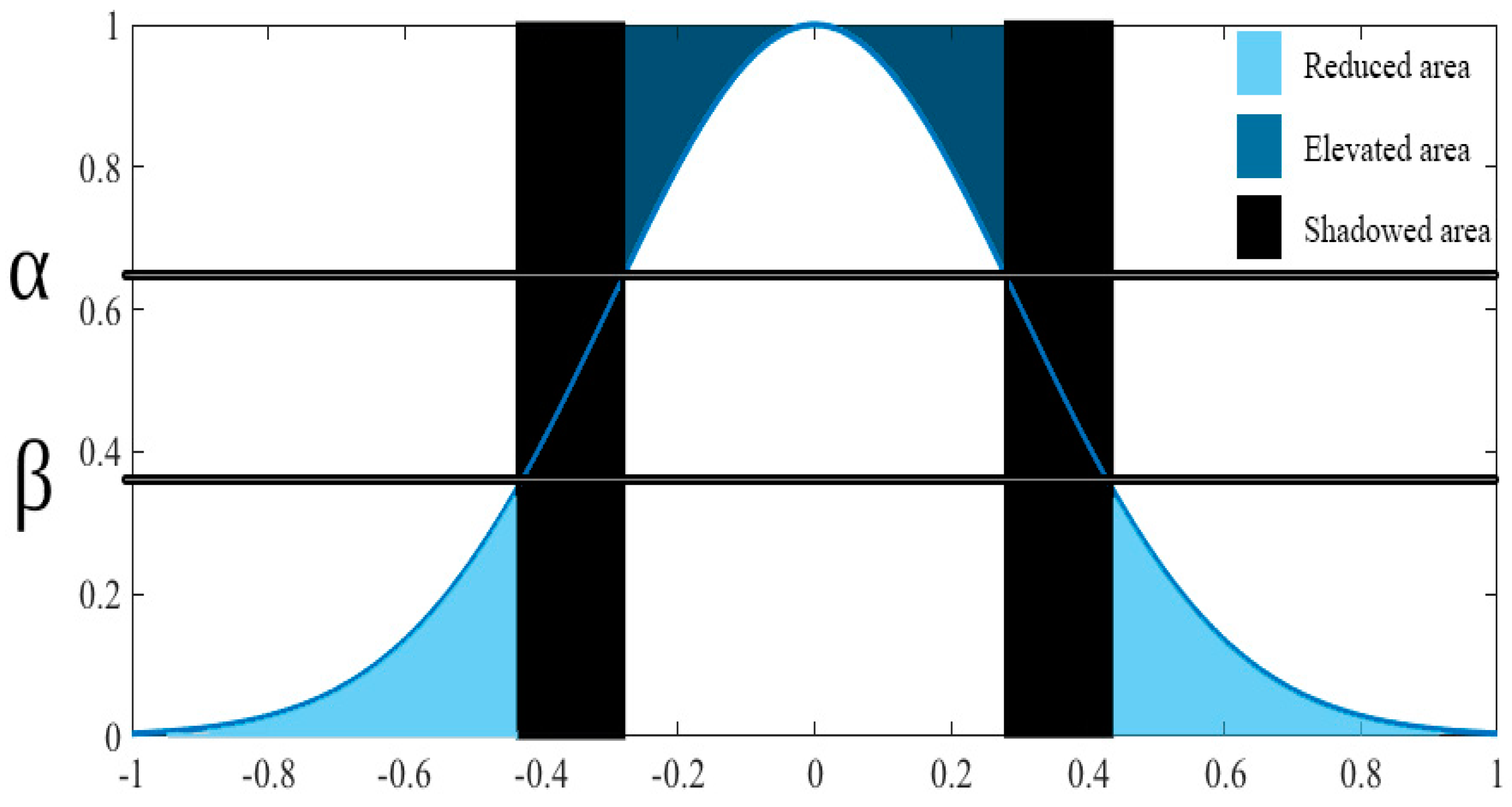
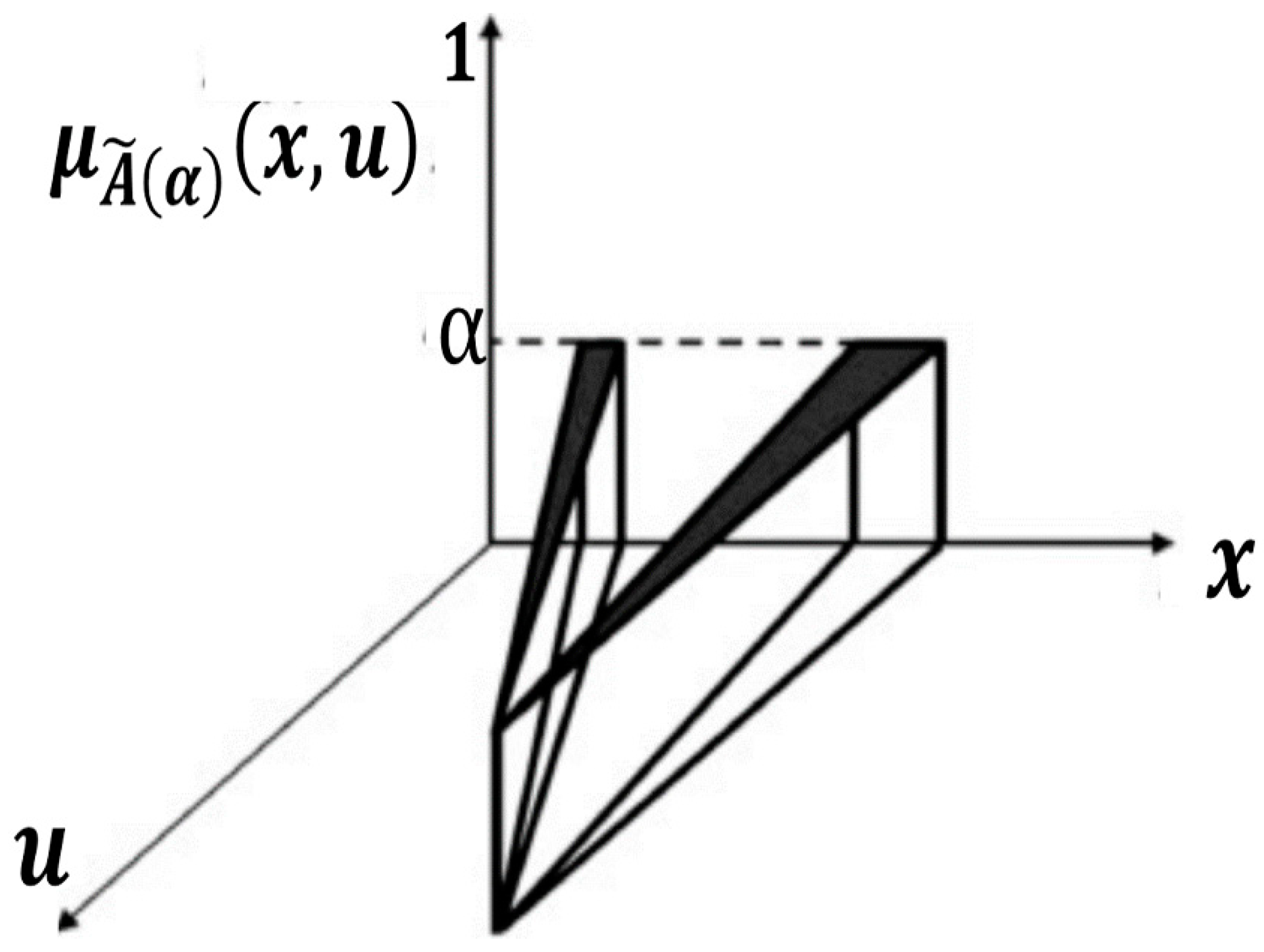
2. Type-2 Fuzzy Systems and Shadowed Sets
- -
- The elevated region for the membership degrees with a value of 1.
- -
- The reduced region for the membership degrees with a value of 0.
- -
- The shaded region with degree of membership in [0, 1].
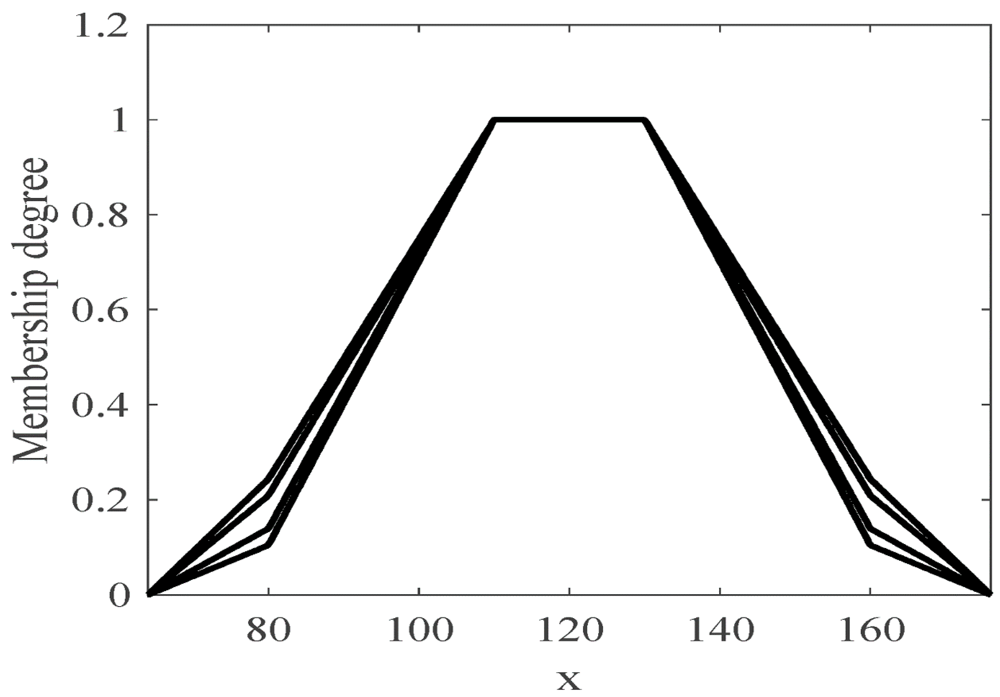
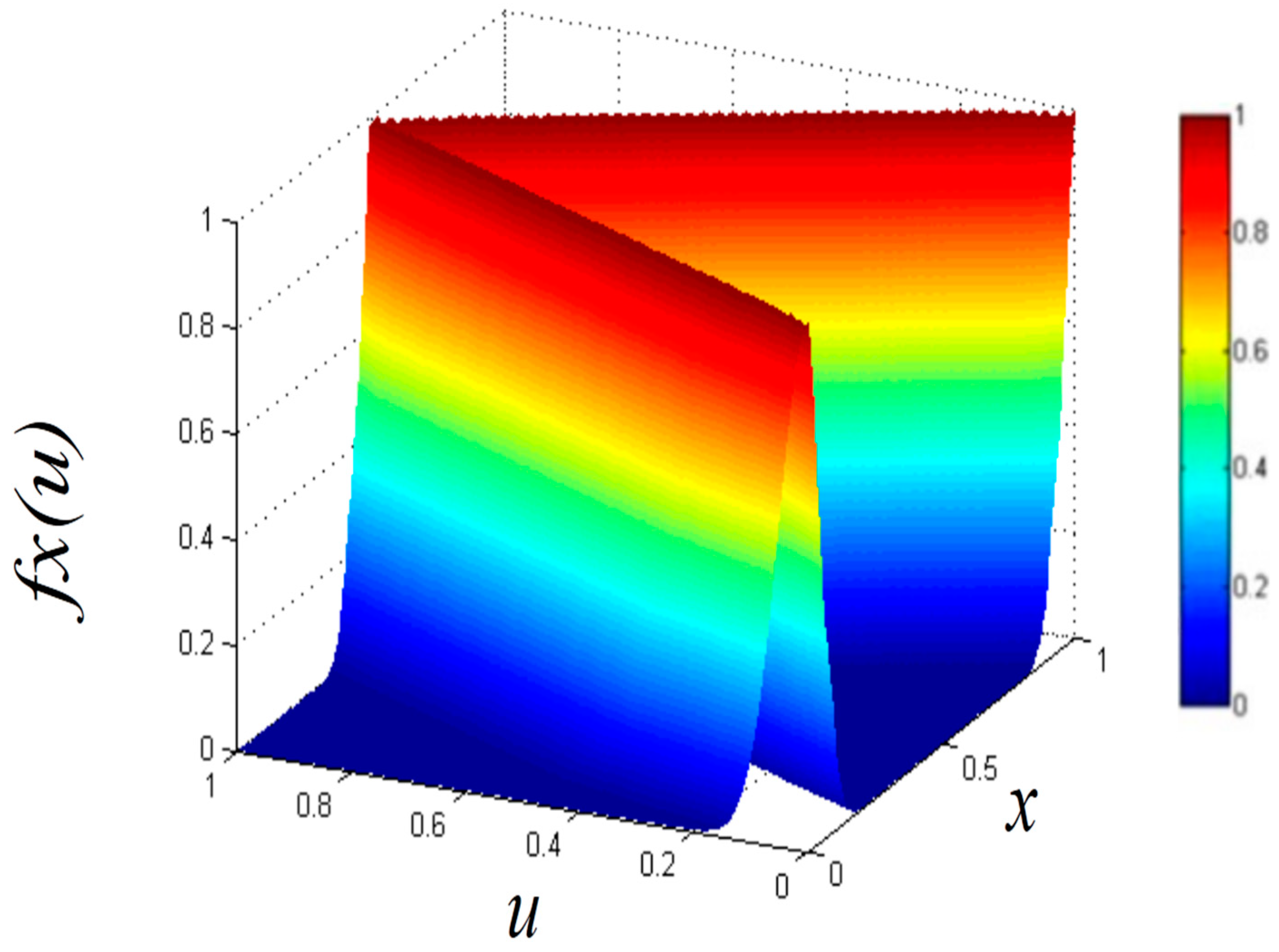
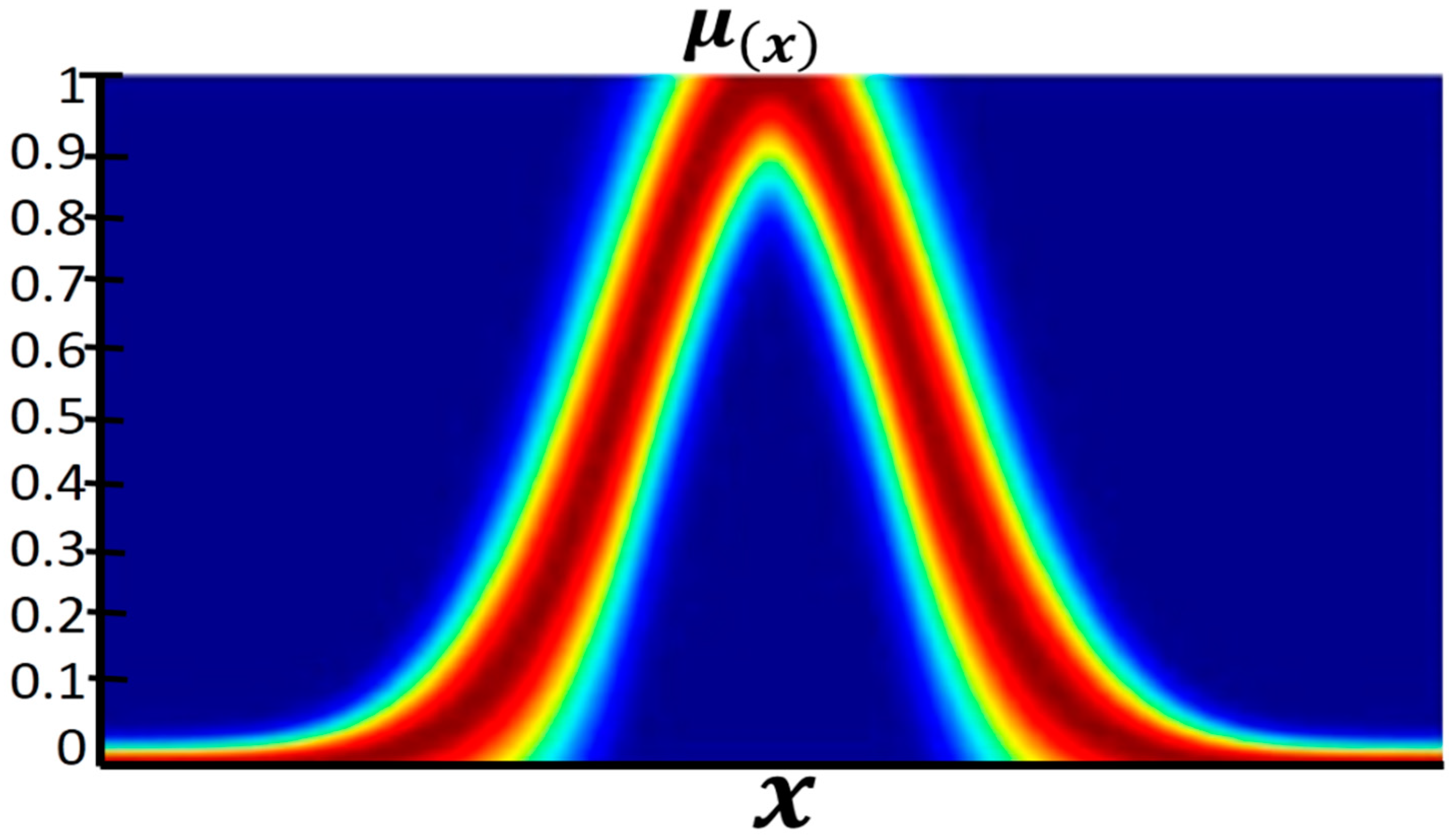
3. General Type-2 Fuzzy Systems
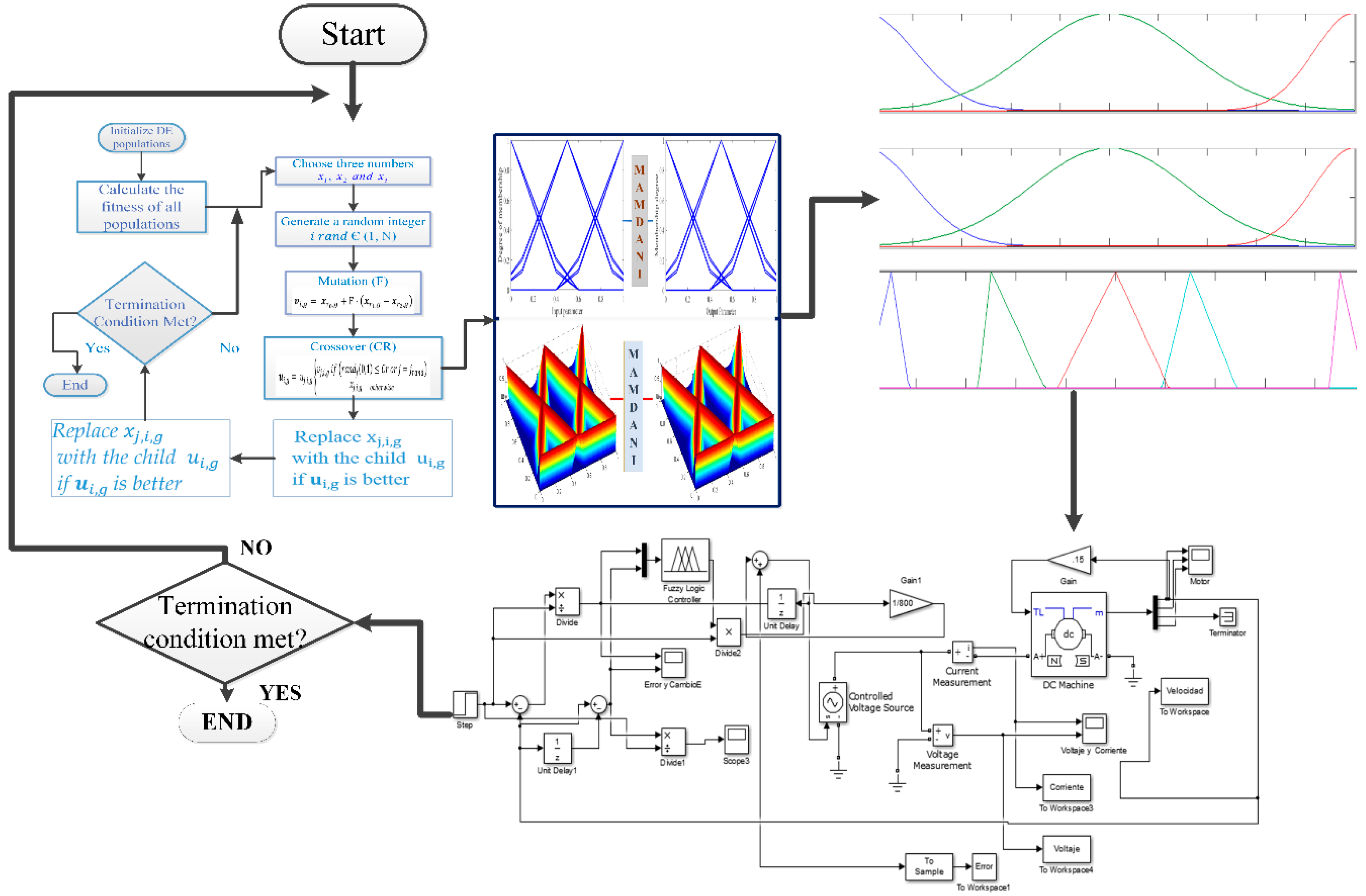
4. Differential Evolution Algorithm
5. Differential Evolution Algorithm with Dynamic Parameter Adaptation
- ➢
- Shadowed Type 2 fuzzy systems
- ➢
- General Type 2 fuzzy systems
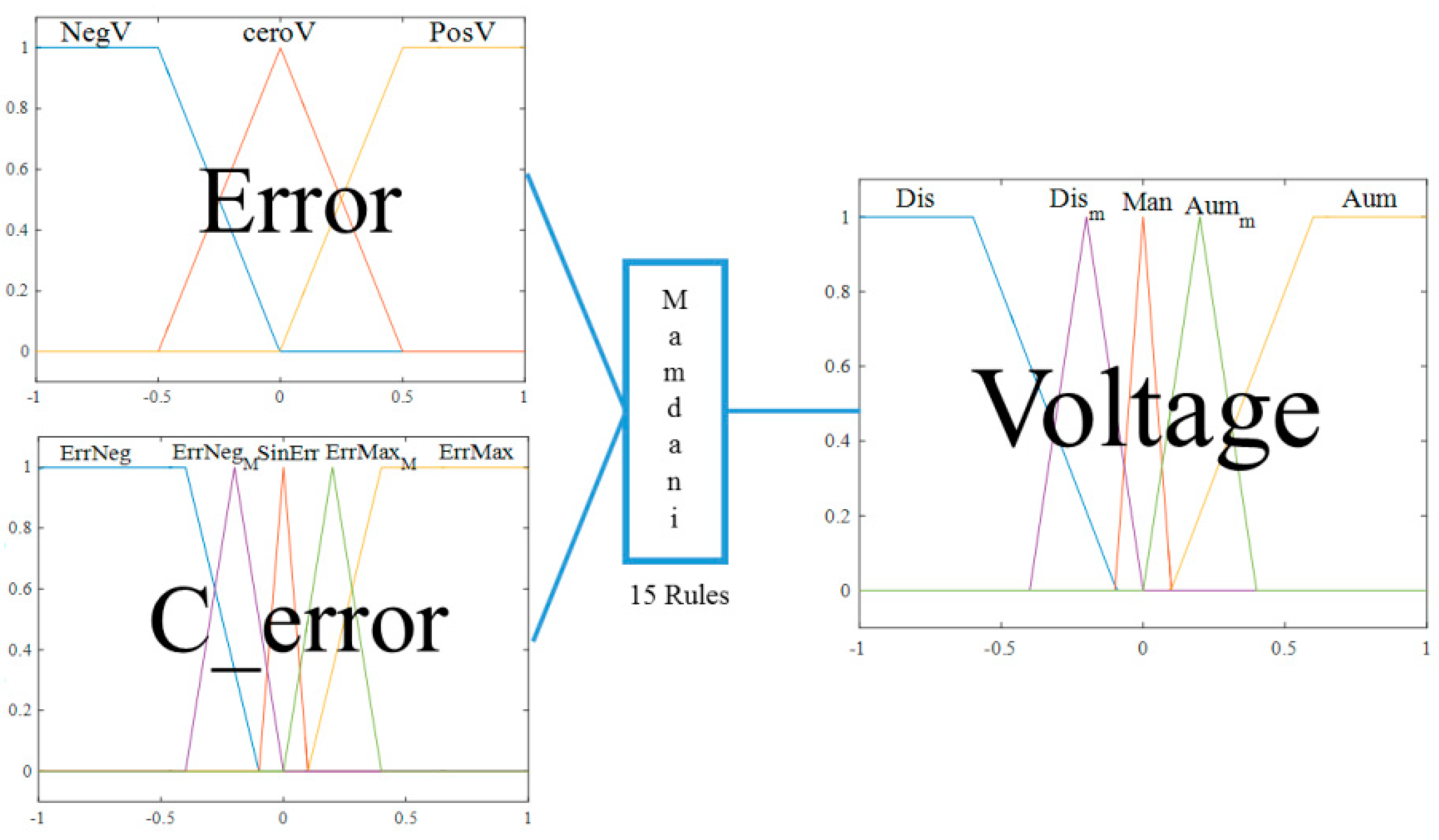
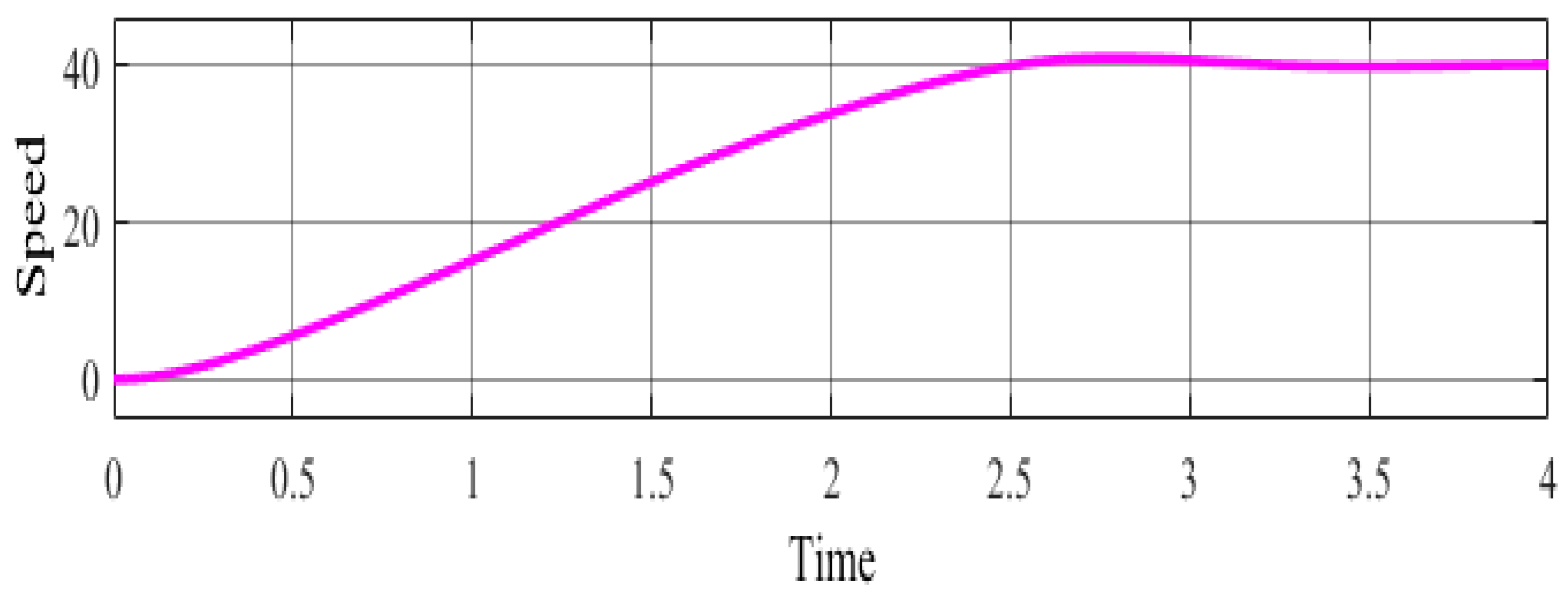
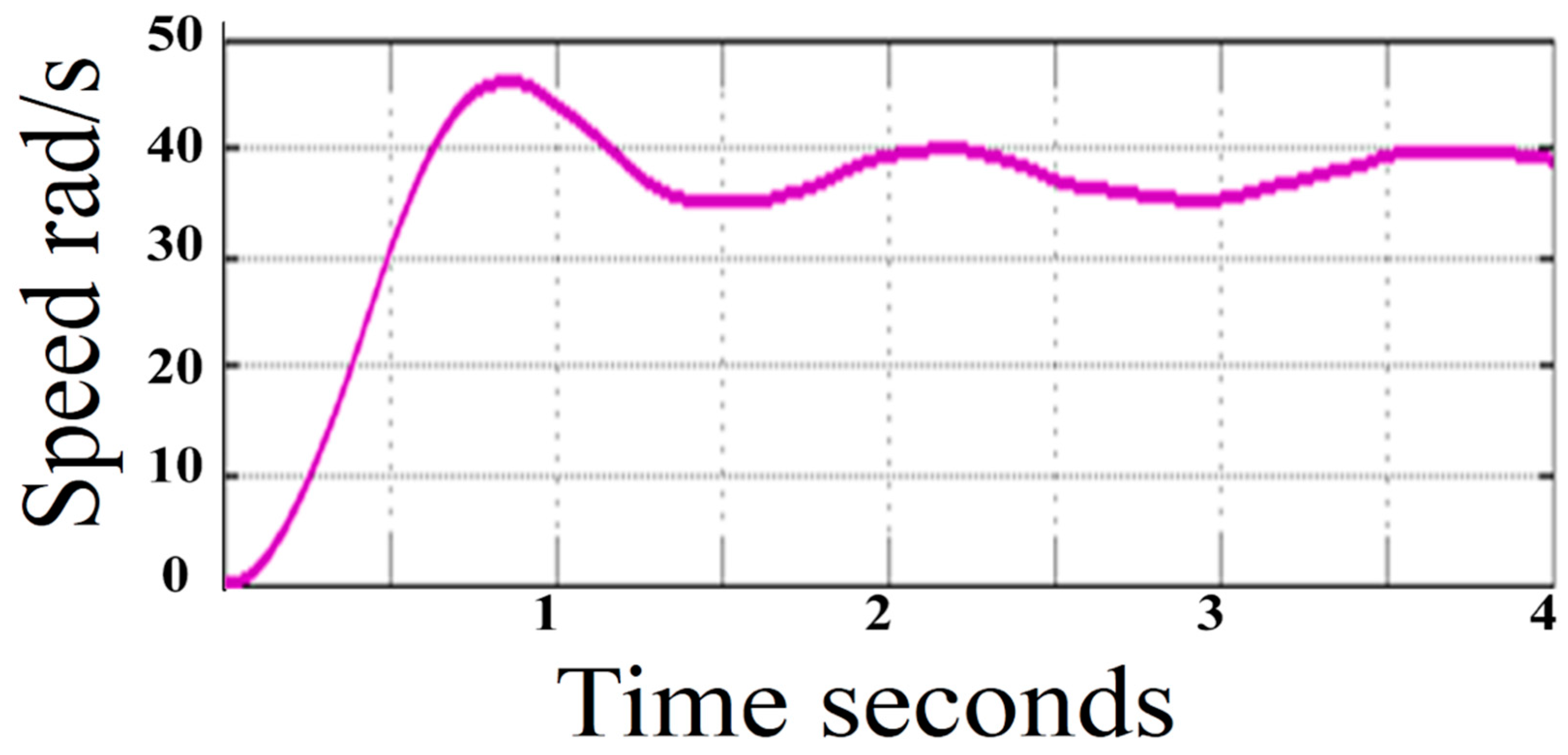
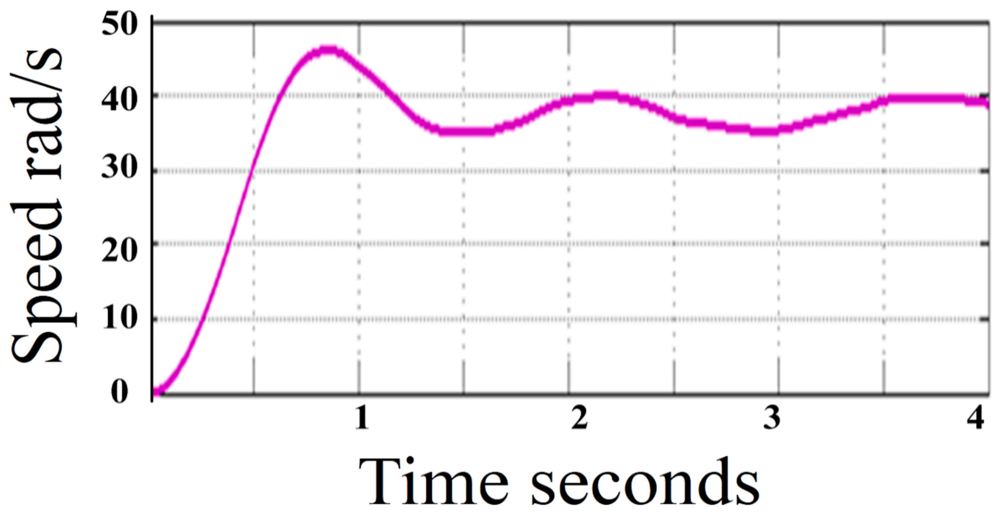
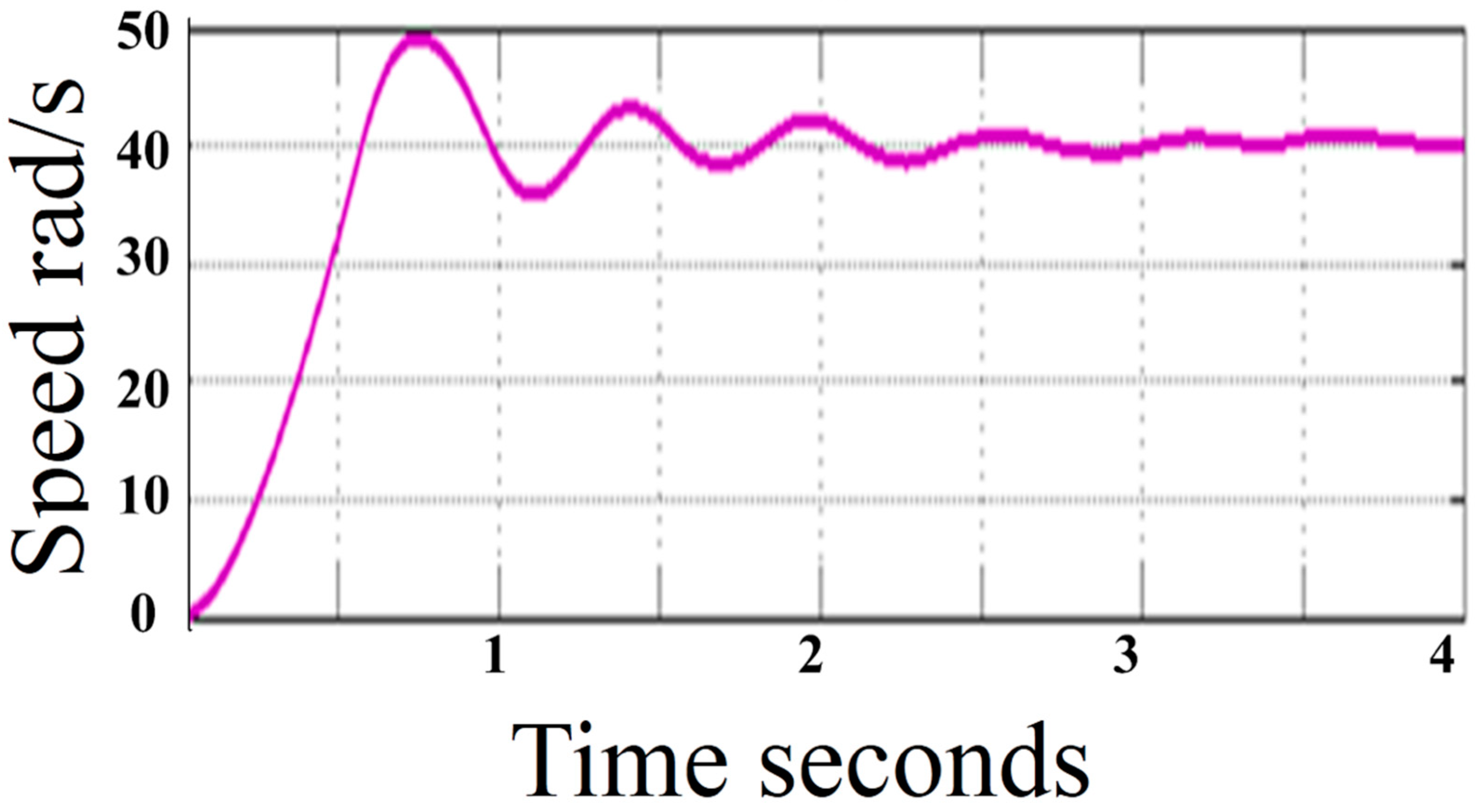
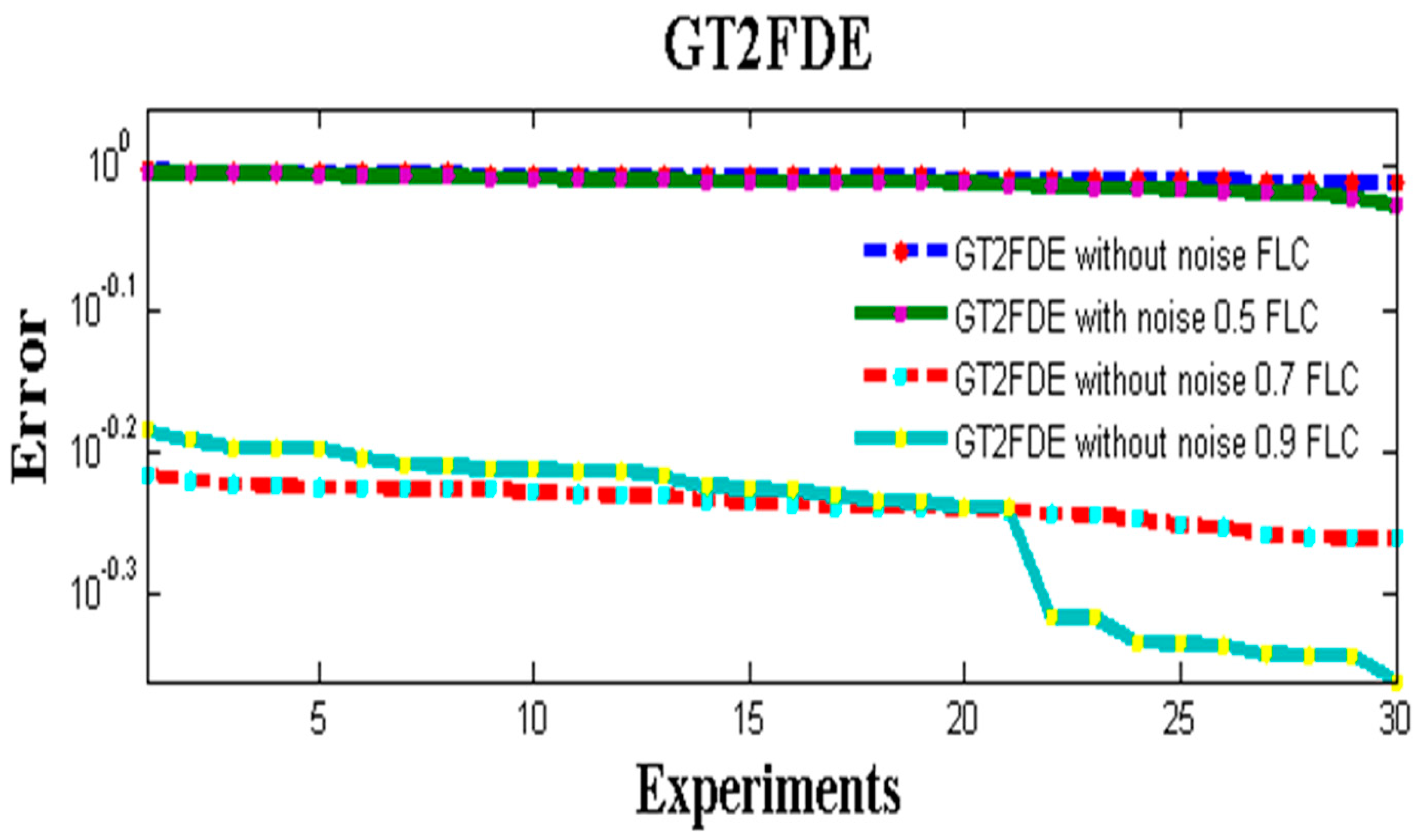
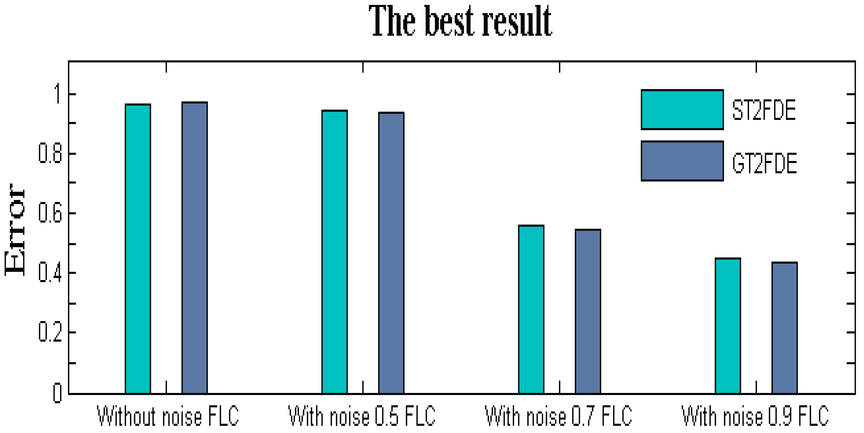
6. Experiments Whit the D.C. Motor Speed Controller
- Ho:
- The results of the GT2FDE methodology without noise and with noise are higher than the methodology ST2FDE without noise and with noise.
- Ha:
- The results of the GT2FDE methodology without noise and with noise are lower than the methodology ST2FDE without noise and with noise.
7. Discussion of Results
8. Conclusions
Author Contributions
Funding
Institutional Review Board Statement
Informed Consent Statement
Data Availability Statement
Conflicts of Interest
Ethical Approval
References
- Castillo, O.; Melin, P.; Valdez, F.; Soria, J.; Ontiveros-Robles, E.; Peraza, C.; Ochoa, P. Shadowed Type-2 Fuzzy Systems for Dynamic Parameter Adaptation in Harmony Search and Differential Evolution Algorithms. Algorithms 2019, 12, 17. [Google Scholar] [CrossRef] [Green Version]
- He, S.; Pan, X.; Wang, Y. A shadowed set-based TODIM method and its application to large-scale group decision making. Inf. Sci. 2021, 544, 135–154. [Google Scholar] [CrossRef]
- Zhang, Q.; Chen, Y.; Yang, J.; Wang, G. Fuzzy Entropy: A More Comprehensible Perspective for Interval Shadowed Sets of Fuzzy Sets. IEEE Trans. Fuzzy Syst. 2019, 28, 3008–3022. [Google Scholar] [CrossRef]
- Li, C.; Yi, J.; Wang, H.; Zhang, G.; Li, J. Interval data driven construction of shadowed sets with application to linguistic word modelling. Inf. Sci. 2020, 507, 503–521. [Google Scholar] [CrossRef]
- William-West, T.O.; Kana, A.F.D.; Ibrahim, A.M. Shadowed set approximation of fuzzy sets based on nearest quota of fuzziness. Ann. Fuzzy Math. Inform. 2019, 17, 133–145. [Google Scholar] [CrossRef]
- Melin, P.; Ontiveros-Robles, E.; Gonzalez, C.I.; Castro, J.R.; Castillo, O. An approach for parameterized shadowed type-2 fuzzy membership functions applied in control applications. Soft Comput. 2018, 23, 3887–3901. [Google Scholar] [CrossRef]
- Bose, A.; Mali, K. A two threshold model for shadowed set with gradual representation of cardinality. In Proceedings of the 2017 14th IEEE India Council International Conference (INDICON), Roorkee, India, 15–17 December 2017; pp. 1–6. [Google Scholar]
- Ontiveros-Robles, E.; Melin, P. A hybrid design of shadowed type-2 fuzzy inference systems applied in diagnosis problems. Eng. Appl. Artif. Intell. 2019, 86, 43–55. [Google Scholar] [CrossRef]
- Pedrycz, W. Shadowed sets: Representing and processing fuzzy sets. IEEE Trans. Syst. Man Cybern. Part. B 1998, 28, 103–109. [Google Scholar] [CrossRef]
- Kirchhof, J.; Krieg, F.; Romer, F.; Ihlow, A.; Osman, A.; Del Galdo, G. Sparse Signal Recovery for ultrasonic detection and reconstruction of shadowed flaws. In Proceedings of the 2017 IEEE International Conference on Acoustics, Speech and Signal Processing (ICASSP), New Orleans, LA, USA, 5–9 March 2017; pp. 816–820. [Google Scholar]
- Zhou, J.; Miao, D.; Gao, C.; Lai, Z.; Yue, X. Constrained three-way approximations of fuzzy sets: From the per-spective of minimal distance. Inf. Sci. 2019, 502, 247–267. [Google Scholar] [CrossRef]
- Yao, Y.; Wang, S.; Deng, X. Constructing shadowed sets and three-way approximations of fuzzy sets. Inf. Sci. 2017, 412–413, 132–153. [Google Scholar] [CrossRef]
- Campagner, A.; Dorigatti, V.; Ciucci, D. Entropy-based shadowed set approximation of intuitionistic fuzzy sets. Int. J. Intell. Syst. 2020, 35, 2117–2139. [Google Scholar] [CrossRef]
- Zhang, Y.; Yao, J. Game theoretic approach to shadowed sets: A three-way tradeoff perspective. Inf. Sci. 2020, 507, 540–552. [Google Scholar] [CrossRef]
- Cai, M.; Li, Q.; Lang, G. Shadowed sets of dynamic fuzzy sets. Granul. Comput. 2016, 2, 85–94. [Google Scholar] [CrossRef]
- Zhou, J.; Gao, C.; Pedrycz, W.; Lai, Z.; Yue, X. Constrained shadowed sets and fast optimization algorithm. Int. J. Intell. Syst. 2019, 34, 2655–2675. [Google Scholar] [CrossRef]
- Zhang, Q.; Gao, M.; Zhao, F.; Wang, G. Fuzzy-entropy-based Game Theoretic Shadowed Sets: A Novel Game Perspective From Uncertainty. IEEE Trans. Fuzzy Syst. 2020, 1, 28. [Google Scholar]
- Wang, H.; He, S.; Pan, X.; Li, C. Shadowed Sets-Based Linguistic Term Modeling and Its Application in Multi-Attribute Decision-Making. Symmetry 2018, 10, 688. [Google Scholar] [CrossRef] [Green Version]
- Mohammadzadeh, A.; Sabzalian, M.H.; Ahmadian, A.; Nabipour, N. A dynamic general type-2 fuzzy system with optimized secondary membership for online frequency regulation. ISA Trans. 2021, 112, 150–160. [Google Scholar] [CrossRef] [PubMed]
- Pal, S.S.; Kar, S. A Hybridized Forecasting Method Based on Weight Adjustment of Neural Network Using Generalized Type-2 Fuzzy Set. Int. J. Fuzzy Syst. 2019, 21, 308–320. [Google Scholar] [CrossRef]
- Bernal, E.; Castillo, O.; Soria, J.; Valdez, F. Parameter Adaptation in the Imperialist Competitive Algorithm Using Generalized Type-2 Fuzzy Logic. In Econometrics for Financial Applications; Springer Science and Business Media LLC: Berlin, Germany, 2020; pp. 3–10. [Google Scholar]
- Ochoa, P.; Castillo, O.; Soria, J. Optimization of fuzzy controller design using a Differential Evolution algorithm with dynamic parameter adaptation based on Type-1 and Interval Type-2 fuzzy systems. Soft Comput. 2019, 24, 193–214. [Google Scholar] [CrossRef]
- Mittal, K.; Jain, A.; Vaisla, K.S.; Castillo, O.; Kacprzyk, J. A comprehensive review on type 2 fuzzy logic applications: Past, present and future. Eng. Appl. Artif. Intell. 2020, 95, 103916. [Google Scholar] [CrossRef]
- Kaur, P.; Gosain, A. GT2FS-SMOTE: An Intelligent Oversampling Approach Based Upon General Type-2 Fuzzy Sets to Detect Web Spam. Arab. J. Sci. Eng. 2021, 46, 3033–3050. [Google Scholar] [CrossRef]
- Cherif, S.; Baklouti, N.; Hagras, H.; Alimi, A.M. Novel Intuitionistic Based Interval Type-2 Fuzzy Similarity Measures with Application to Clustering. IEEE Trans. Fuzzy Syst. 2021, 1. [Google Scholar] [CrossRef]
- Zhang, Z.; Niu, Y.; Song, J. Input-to-State Stabilization of Interval Type-2 Fuzzy Systems Subject to Cyberattacks: An Observer-Based Adaptive Sliding Mode Approach. IEEE Trans. Fuzzy Syst. 2020, 28, 190–203. [Google Scholar] [CrossRef]
- Yang, Y.; Niu, Y.; Zhang, Z. Dynamic event-triggered sliding mode control for interval Type-2 fuzzy systems with fading channels. ISA Trans. 2021, 110, 53–62. [Google Scholar] [CrossRef] [PubMed]
- Zhao, T.; Chen, Y.; Dian, S.; Guo, R.; Li, S. General Type-2 Fuzzy Gain Scheduling PID Controller with Application to Power-Line Inspection Robots. Int. J. Fuzzy Syst. 2019, 22, 181–200. [Google Scholar] [CrossRef]
- Shahparast, H.; Mansoori, E.G. Developing an online general type-2 fuzzy classifier using evolving type-1 rules. Int. J. Approx. Reason. 2019, 113, 336–353. [Google Scholar] [CrossRef]
- Gonzalez, C.I.; Melin, P.; Castillo, O.; Juarez, D.; Castro, J.R. Toward General Type-2 Fuzzy Logic Systems Based on Shadowed Sets. In Advances in Intelligent Systems and Computing; Springer Science and Business Media LLC: Berlin, Germany, 2018; pp. 131–142. [Google Scholar]
- Jafari, P.; Teshnehlab, M.; Tavakoli-Kakhki, M. Adaptive type-2 fuzzy system for synchronisation and stabilisation of chaotic non-linear fractional order systems. IET Control. Theory Appl. 2018, 12, 183–193. [Google Scholar] [CrossRef]
- Su, Z.; Hu, D.; Yu, X. General interval approach for encoding words into interval type-2 fuzzy sets based on normal distribution and free parameter. Soft Comput. 2018, 23, 8187–8206. [Google Scholar] [CrossRef]
- Zadeh, L.A. Fuzzy Sets. Inf. Control 1964, 8, 338–353. [Google Scholar] [CrossRef] [Green Version]
- Wagner, C.; Hagras, H. Toward General Type-2 Fuzzy Logic Systems Based on zSlices. IEEE Trans. Fuzzy Syst. 2010, 18, 637–660. [Google Scholar] [CrossRef]
- Coupland, S.; John, R. Geometric Type-1 and Type-2 Fuzzy Logic Systems. IEEE Trans. Fuzzy Syst. 2007, 15, 3–15. [Google Scholar] [CrossRef]
- Mendel, J.M.; Liu, F.; Zhai, D. αα-Plane Representation for Type-2 Fuzzy Sets: Theory and Applications. IEEE Trans. Fuzzy Syst. 2009, 17, 1189–1207. [Google Scholar] [CrossRef]
- Mendel, J.M.; John, R.; Liu, F. Interval Type-2 Fuzzy Logic Systems Made Simple. IEEE Trans. Fuzzy Syst. 2006, 14, 808–821. [Google Scholar] [CrossRef] [Green Version]
- Wijayasekara, D.; Linda, O.; Manic, M. Shadowed Type-2 Fuzzy Logic Systems. In Proceedings of the IEEE Symposium on Advances in Type-2 Fuzzy Logic Systems (T2FUZZ), Singapore, 16–19 April 2013; pp. 15–22. [Google Scholar]
- Pedrycz, W. From fuzzy sets to shadowed sets: Interpretation and computing. Int. J. Intell. Syst. 2009, 24, 48–61. [Google Scholar] [CrossRef]
- Pedrycz, W.; Song, M. Granular fuzzy models: A study in knowledge management in fuzzy modeling. Int. J. Approx. Reason. 2012, 53, 1061–1079. [Google Scholar] [CrossRef] [Green Version]
- Pedrycz, W.; Vukovich, G. Granular computing in the development of fuzzy controllers. Int. J. Intell. Syst. 1999, 14, 419–447. [Google Scholar] [CrossRef]
- Melin, P.; Gonzalez, C.I.; Castro, J.R.; Mendoza, O.; Castillo, O. Edge-Detection Method for Image Processing Based on Generalized Type-2 Fuzzy Logic. IEEE Trans. Fuzzy Syst. 2014, 22, 1515–1525. [Google Scholar] [CrossRef]
- Sánchez, M.A.; Castro, J.R.; Castillo, O. Formation of general type-2 Gaussian membership functions based on the information granule numerical evidence. In 2013 IEEE Workshop on Hybrid Intelligent Models and Applications (HIMA); Institute of Electrical and Electronics Engineers (IEEE): Piscataway, NJ, USA, 2013; pp. 1–6. [Google Scholar]
- Carvajal, O.; Melin, P.; Miramontes, I.; Prado-Arechiga, G. Optimal design of a general type-2 fuzzy classifier for the pulse level and its hardware implementation. Eng. Appl. Artif. Intell. 2021, 97, 104069. [Google Scholar] [CrossRef]
- Price, K.; Storn, R.M.; Lampinen, J.A. Differential Evolution: A Practical Approach to Global Optimization; Springer Science & Business Media: Berlin, Germany, 2006. [Google Scholar]
- Castillo, O.; Valdez, F.; Soria, J.; Yoon, J.H.; Geem, Z.W.; Peraza, C.; Ochoa, P.; Amador-Angulo, L. Optimal Design of Fuzzy Systems Using Differential Evolution and Harmony Search Algorithms with Dynamic Parameter Adaptation. Appl. Sci. 2020, 10, 6146. [Google Scholar] [CrossRef]
- Ochoa, P.; Castillo, O.; Soria, J. High-Speed Interval Type-2 Fuzzy System for Dynamic Crossover Parameter Ad-aptation in Differential Evolution and Its Application to Controller Optimization. Int. J. Fuzzy Syst. 2020, 22, 414–427. [Google Scholar] [CrossRef]
- Castillo, O.; Ochoa, P.; Soria, J. Differential Evolution Algorithm with Type-2 Fuzzy Logic. For Dynamic Parameter Adap-tation with Application to Intelligent Control.; Springer Nature: Berlin, Germany, 2020. [Google Scholar]
- Amador-Angulo, L.; Castillo, O.; Peraza, C.; Ochoa, P. An Efficient Chicken Search Optimization Algorithm for the Optimal Design of Fuzzy Controllers. Axioms 2021, 10, 30. [Google Scholar] [CrossRef]
- Ontiveros, E.; Melin, P.; Castillo, O. Impact Study of the Footprint of Uncertainty in Control Applications Based on Interval Type-2 Fuzzy Logic Controllers. Fuzzy Logic. Augmentation of Neural and Optimization Algorithms: Theoretical Aspects and Real Applications; Springer: Berlin, Germany, 2018; pp. 181–197. [Google Scholar]
- Castillo, O.; Melin, P.; Ontiveros-Robles, E.; Peraza, C.; Ochoa, P.; Valdez, F.; Soria, J. A high-speed interval type 2 fuzzy system approach for dynamic parameter adaptation in metaheuristics. Eng. Appl. Artif. Intell. 2019, 85, 666–680. [Google Scholar] [CrossRef]
- Ontiveros-Robles, E.; Melin, P.; Castillo, O. High order α-planes integration: A new approach to computational cost reduction of General Type-2 Fuzzy Systems. Eng. Appl. Artif. Intell. 2018, 74, 186–197. [Google Scholar] [CrossRef]
- Olivas, F.; Valdez, F.; Castillo, O.; Melin, P. Dynamic parameter adaptation in particle swarm optimization using interval type-2 fuzzy logic. Soft Comput. 2014, 20, 1057–1070. [Google Scholar] [CrossRef]
- Olivas, F.; Valdez, F.; Melin, P.; Sombra, A.; Castillo, O. Interval type-2 fuzzy logic for dynamic parameter adaptation in a modified gravitational search algorithm. Inf. Sci. 2019, 476, 159–175. [Google Scholar] [CrossRef]
- Castillo, O.; Amador-Angulo, L. A generalized type-2 fuzzy logic approach for dynamic parameter adaptation in bee colony optimization applied to fuzzy controller design. Inf. Sci. 2018, 460–461, 476–496. [Google Scholar] [CrossRef]
- Rubio, E.; Castillo, O.; Valdez, F.; Melin, P.; Gonzalez, C.I.; Martinez, E.G. An Extension of the Fuzzy Possibilistic Clustering Algorithm Using Type-2 Fuzzy Logic Techniques. Adv. Fuzzy Syst. 2017, 2017, 1–23. [Google Scholar] [CrossRef] [Green Version]


| Generation | F | ||
|---|---|---|---|
| Low | Medium | High | |
| Low | − | − | Low |
| Medium | − | Medium | − |
| High | High | − | − |
| Generalized Type-2 Fuzzy Logic Sets | |
|---|---|
| Low | |
| Medium | |
| High | |
| No. | Inputs | Output | |
|---|---|---|---|
| Error | Change in Error | Voltage | |
| 1 | NegV | ErrNeg | Dis |
| 2 | NegV | SinErr | Dis |
| 3 | NegV | ErrMax | Dis_m |
| 4 | ZeroV | ErrNeg | Aum_m |
| 5 | ZeroV | ErrMax | Dis_m |
| 6 | PosV | ErrNeg | Aum_m |
| 7 | PosV | SinErr | Aum |
| 8 | PosV | ErrMax | Aum |
| 9 | ZeroV | SinErr | Man |
| 10 | NegV | ErrNeg_M | Dis |
| 11 | ZeroV | ErrNeg_M | Aum_m |
| 12 | PosV | ErrNeg_M | Aum |
| 13 | PosV | ErrMax_M | Aum |
| 14 | ZeroV | ErrMax_M | Dis_m |
| 15 | NegV | ErrMax_M | Dis |
| Parameters | ST2FDE and GT2FDE |
|---|---|
| Population | 50 |
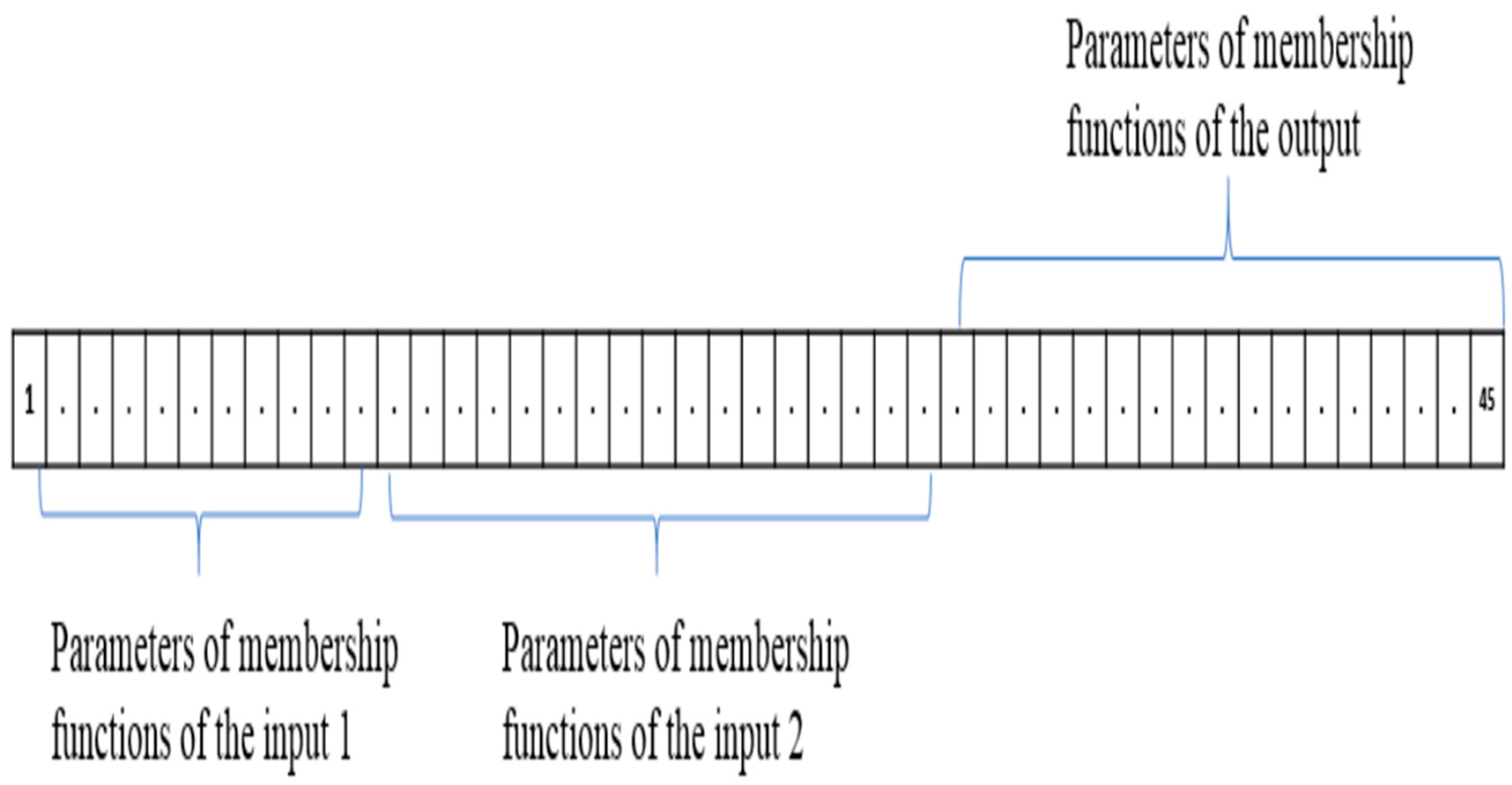
| Dimensions | 45 |
| Generations | 30 |
| Number of experiments | 30 |
| F | Dynamic |
| Cr | 0.3 |
| ST2FDE | ||||
|---|---|---|---|---|
| Method | ST2FDE without Noise FLC | ST2FDE with Noise 0.5 FLC | ST2FDE with Noise 0.7 FLC | ST2FDE with Noise 0.9 FLC |
| Best | 9.66 | 9.41 | 5.59 | 4.52 |
| Worst | 9.98 | 9.96 | 6.11 | 6.56 |
| Average | 9.84 | 9.73 | 5.86 | 5.81 |
| Std. | 8.45 | 1.17 | 1.40 | 6.13 |
| GT2FDE | ||||
|---|---|---|---|---|
| Method | GT2FDE without Noise FLC | GT2FDE with Noise 0.5 FLC | GT2FDE with Noise 0.7 FLC | GT2FDE with Noise 0.9 FLC |
| Best | 9.73 | 9.38 | 5.48 | 4.35 |
| Worst | 9.95 | 9.91 | 6.08 | 6.53 |
| Average | 9.85 | 9.75 | 5.79 | 5.51 |
| Std. | 5.88 | 1.25 | 1.70 | 7.46 |
| Parameter | Value |
|---|---|
| Level of Confidence | 95% |
| Alpha | 0.05% |
| Ha | µ1 < µ2 |
| H0 | µ1 ≥ µ2 |
| Critical Value | −1.645 |
| Statistical Tests | ||||
|---|---|---|---|---|
| Case Study | Z Value | Evidence | ||
| Speed control in a D.C. Motor | GT2FDE without FCL noise | ST2FDE without FCL noise | 0.5321 | Not Significant |
| GT2FDE with FCL 0.5 noise | ST2FDE without FCL 0.5 noise | 0.6398 | Not Significant | |
| GT2FDE with FCL 0.7 noise | ST2FDE without FCL 0.7 noise | −1.7410 | Significant | |
| GT2FDE with FCL 0.9 noise | ST2FDE without FCL 0.9 noise | −1.7018 | Significant | |
| D.C. Motor Speed Controller | RMSE | Method | Best |
| Original DE | 4.72 | ||
| DEFIS 1 | 4.57 | ||
| DEFIS 2 | 4.80 | ||
| DEFIS 3 | 2.36 | ||
| Original HS | 4.72 | ||
| HSFIS 1 | 4.57 | ||
| HSFIS 2 | 4.80 | ||
| HSFIS 3 | 2.36 | ||
| GT2FDE with noise 0.9 FLC | 4.35 × 10−02 |
Publisher’s Note: MDPI stays neutral with regard to jurisdictional claims in published maps and institutional affiliations. |
© 2021 by the authors. Licensee MDPI, Basel, Switzerland. This article is an open access article distributed under the terms and conditions of the Creative Commons Attribution (CC BY) license (https://creativecommons.org/licenses/by/4.0/).
Share and Cite
Ochoa, P.; Castillo, O.; Melin, P.; Soria, J. Differential Evolution with Shadowed and General Type-2 Fuzzy Systems for Dynamic Parameter Adaptation in Optimal Design of Fuzzy Controllers. Axioms 2021, 10, 194. https://0-doi-org.brum.beds.ac.uk/10.3390/axioms10030194
Ochoa P, Castillo O, Melin P, Soria J. Differential Evolution with Shadowed and General Type-2 Fuzzy Systems for Dynamic Parameter Adaptation in Optimal Design of Fuzzy Controllers. Axioms. 2021; 10(3):194. https://0-doi-org.brum.beds.ac.uk/10.3390/axioms10030194
Chicago/Turabian StyleOchoa, Patricia, Oscar Castillo, Patricia Melin, and José Soria. 2021. "Differential Evolution with Shadowed and General Type-2 Fuzzy Systems for Dynamic Parameter Adaptation in Optimal Design of Fuzzy Controllers" Axioms 10, no. 3: 194. https://0-doi-org.brum.beds.ac.uk/10.3390/axioms10030194