Co-Training Method Based on Semi-Decoupling Features for MOOC Learner Behavior Prediction

Abstract

Facing the problem of massive unlabeled data and limited labeled samples, semi-supervised learning is favored, especially co-training. Standard co-training requires sufficiently redundant and conditionally independent dual views; however, in fact, few dual views exist that satisfy this condition. To solve this problem, we propose a co-training method based on semi-decoupling features, that is, semi-decoupling features based on a known single view and then constructing independent and redundant dual views: (1) take a small number of important features as shared features of the dual views according to the importance of the features; (2) separate the remaining features one by one or in small batches according to the correlation between the features to make “divergent” features of the dual views; (3) combine the shared features and the “divergent” features to construct dual views. In this paper, the experimental dataset was from the edX dataset jointly released by Harvard University and MIT; the evaluation metrics adopted F1, Precision, and Recall. The analysis methods included three experiments: multiple models, iterations, and hyperparameters. The experimental results show that the effect of this model on MOOC learner behavior prediction was better than the other models, and the best prediction result was obtained in iteration 2. These all verify the effectiveness and superiority of this algorithm and provide a scientific and feasible reference for the development of the future education industry.

1. Introduction

The basic purpose of machine learning is to learn useful knowledge from data and to use inductive laws to analyze and predict future results. Machine learning methods are mainly divided into supervised learning, unsupervised learning, and semi-supervised learning [1,2]. Among them, supervised learning needs a large number of labeled data [3,4,5,6], while unsupervised learning does not need any prior knowledge, but it clusters similar samples into one category by fitting the internal distribution of unlabeled data [7,8,9,10,11,12]. With the rapid development of technology for data collection and storage, the acquisition of unlabeled data has become quite easy [3], but labeled data often require a lot of manual intervention and, in some cases, even professional advice. Thus, in most scenarios, the amount of labeled data are still insufficient for many practical applications. However, if only a small amount of labeled data are used, it is easy to cause an overfitting problem for the learning model and leads to a lack of good generalization ability. The challenge of using a large number of idle unlabeled samples to effectively enhance the generalization of the model has become one of the hotspots in the machine learning field [13,14].

Semi-supervised learning is an important research hotspot that combines supervised learning with unsupervised learning [15]. The aim is to use massive unlabeled data and limited labeled data to train the model, learn the potential information of the unlabeled data, ensure the good performance of the model on the basis of supervised learning, and improve the generalization of the model [16,17]. According to different learning methods, it is mainly divided into four categories: a generative model-based method [18], a graph-based method [19], a semi-supervised support vector machine-based method [20], and a co-training algorithm [21,22].

Compared to other methods, co-training is simpler and more efficient. It must be assumed that there are sufficiently redundant and conditionally independent dual views in the problem domain. Here, “sufficiently redundant” means that each view contains enough information to produce an optimal model, and “conditionally independent” means that under the category label of given data, the two views are independent and do not interfere with each other. By using the dual view, two classifiers are trained from different perspectives, and then the data with the higher confidence are selected as a pseudo-label sample to add another view to achieve complementary advantages. They learn from each other and make progress together until they no longer change or reach a preset iteration.

Among the existing co-training studies, there are several models based on different learning algorithms, different data adoptions, different parameter settings, and different multi-view acquisitions such as tri-training and random segmentation. They all enhance the classification performance of co-training and reveal the intrinsic mechanism. However, the data obtained by these models’ algorithms still suffer from conflicting feature attributes with poor relevance, difficulty in optimizing important features, and the limitations of irrelevant features in real application scenarios. These all directly affect the performance of classifiers and, so far, there has been no research to address these issues in depth. To solve this situation, we propose a co-training method based on semi-decoupling feature: segmentation of a single view based on feature attributes. The main steps are as follows:

(1)

Calculate the feature importance of the dataset and rank them, and then select a number of the most important features as the shared features of the dual views;

(2)

Calculate the correlation coefficients between features, process the remaining features according to the correlation coefficients, and then add them to the dual views as other features. While not reducing the data and ensuring the sufficiency of the data, separate the two views as independently as possible according to the feature correlation and difference;

(3)

Combine shared features and “divergent” features to complete feature semi-decoupling, and then construct independent and redundant dual views for co-training.

This algorithm was tested on the edX dataset released by Harvard University and MIT, evaluated with F1, Precision, and Recall, and analyzed by multiple models, iterations, and hyperparameters. The experiments show that our model obtained better performance on MOOC learner behavior prediction. In addition, they also demonstrated the further effectiveness and superiority of the algorithm that is proposed and implemented in this paper.

In this paper, we aimed to disentangle the independent and redundant dual views on a known single view as much as possible to satisfy the assumptions of standard co-training multiple views, to avoid the problems of conflicting feature attributes and difficulties in optimizing important features, and to improve the performance of the classifier.

2. Related Work

Since 1998, when A. Blum and T. Mitchell first proposed the formal co-training algorithm, co-training has gradually become one of the most important mainstream directions in the field of semi-supervised learning [23]. The existing literature makes further improvements on the standard co-training. On the one hand, it improves co-training for single views and generates multiple sub-learners with differences by different learning algorithms [24], different data adoptions [25], and different parameter settings [26] so that multi-view learning can be accomplished even when the views are not redundant and the view features are not independent. On the other hand, there are also some studies around view segmentation to achieve co-training by differential multi-view acquisition [27].

The co-training model proposed by A. Blum and T. Mitchell first assumes that there are two fully redundant and conditionally independent views in the dataset. They use labeled samples to train different classifiers on these two views, and then select a number of samples with higher confidence from the unlabeled samples. After, those samples are added to each other’s classifier to realize differences and complete an update. In this way, the whole process is continuously iterated until it reaches a certain stop condition. Subsequently, based on different learning algorithms, co-training, tri-training, co-forest, and co-trade variants have been derived [28,29,30]. References [31,32] suggested the tri-training algorithm; it neither requires fully redundant multiple views nor various types of base classifiers but combines semi-supervised learning and integrates learning mechanisms to obtain three labeled training sets by repeatedly sampling from labeled samples and generating three classifiers to achieve prediction on the same unlabeled sample. References [33,34] also proposed the co-forest algorithm, which uses a combination of several classification decision trees to ensure the difference and robustness of each classifier. Unlike the tri-training and co-forest models, the co-trade model follows the standard co-training premise assumptions [35,36]. It uses a data editing technique based on cutting-edge weight statistics to determine the labeling confidence. Then, the pseudo-labeled data with the lowest error rate is selected to join the next round of training data for another classifier. The algorithm provides the exact value of the error rate for each iteration and reduces the introduction of noisy samples during the training process.

There are also some studies around view segmentation, so as to achieve adequate and redundant multi-view acquisition [37,38]. The literature [39] has proposed a random subspace partitioning algorithm, which mainly discusses the influence of the numbers and dimensions of subspaces on the classification performance. The more random the subspaces, the worse the classification performance. The main reason for this is that the quality of the optimal subspace selection is limited by the irrelevant features. The literature [40] suggests a view adequacy-based segmentation algorithm, which is based on attribute simplification in rough set theory. In this algorithm, high-dimensional data are reduced to low-dimensional subspaces, and important attributes are added sequentially until the current mutual information and the original mutual information are equal. Reference [41] proposed a view independence-based segmentation algorithm. The core idea is to use the maxInd algorithm of graph, add mutual information index to measure the amount of information sharing between features, and realize multi-view acquisition. The literature [42] suggests an automatic segmentation algorithm, mainly by initializing the weights of two classifiers, and then the two classifiers split the single view based on the optimal loss function to obtain two new views.

3. Materials and Methods

3.1. Co-Training

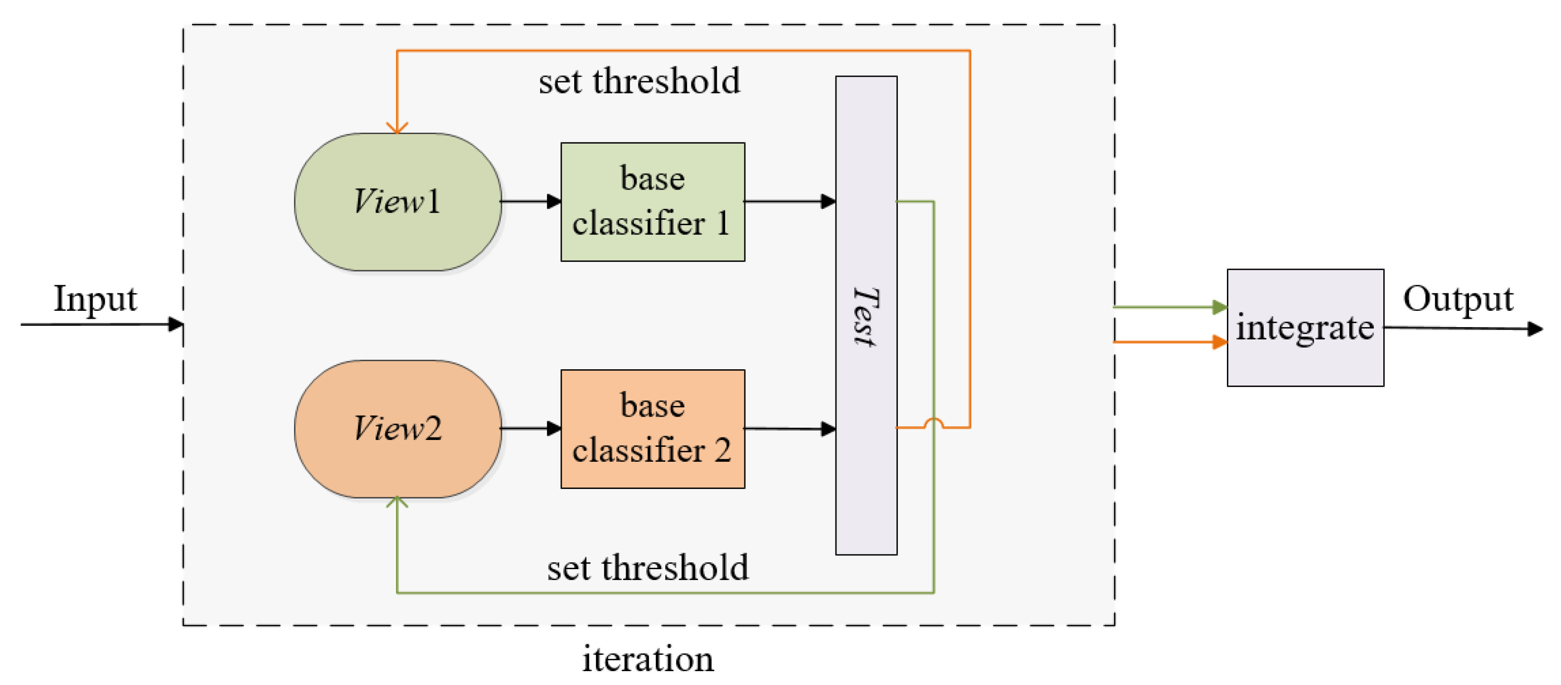
In this section, we briefly review co-training and the relevant concepts. Co-training was first introduced in 1998, which was originally designed for independent redundant “multi-view” data and was a kind of semi-supervised learning method based on “divergence”. The key to the algorithm is to assume that there are two independent redundant views. First, two classifiers with large differences are trained and the unlabeled sample set is classified. Subsequently, the positive and negative samples, respectively, with high confidence or that meet the set threshold are labeled, and then they complement each other by adding these samples to form a new view. Lastly, the filtered pseudo-label samples are deleted from the unlabeled sample set. Iterations occur, as described above, until the unlabeled sample set is empty or meets a specific stop criterion.

In Figure 1, the process of co-training is described. View1 and View2 denote the known view 1 and known view 2, respectively; Test denotes the test set or unlabeled sampling set.

3.2. Semi-Decoupled Features

In this section, we introduce the research background of semi-decoupled features and the specific process of the algorithm. The feature set itself cannot be separated naturally. Therefore, it is difficult to ensure the independence between the views if it is randomly divided. That is, there is still a strong correlation between multiple views, which makes it difficult to realize the difference complementing of the independent views.

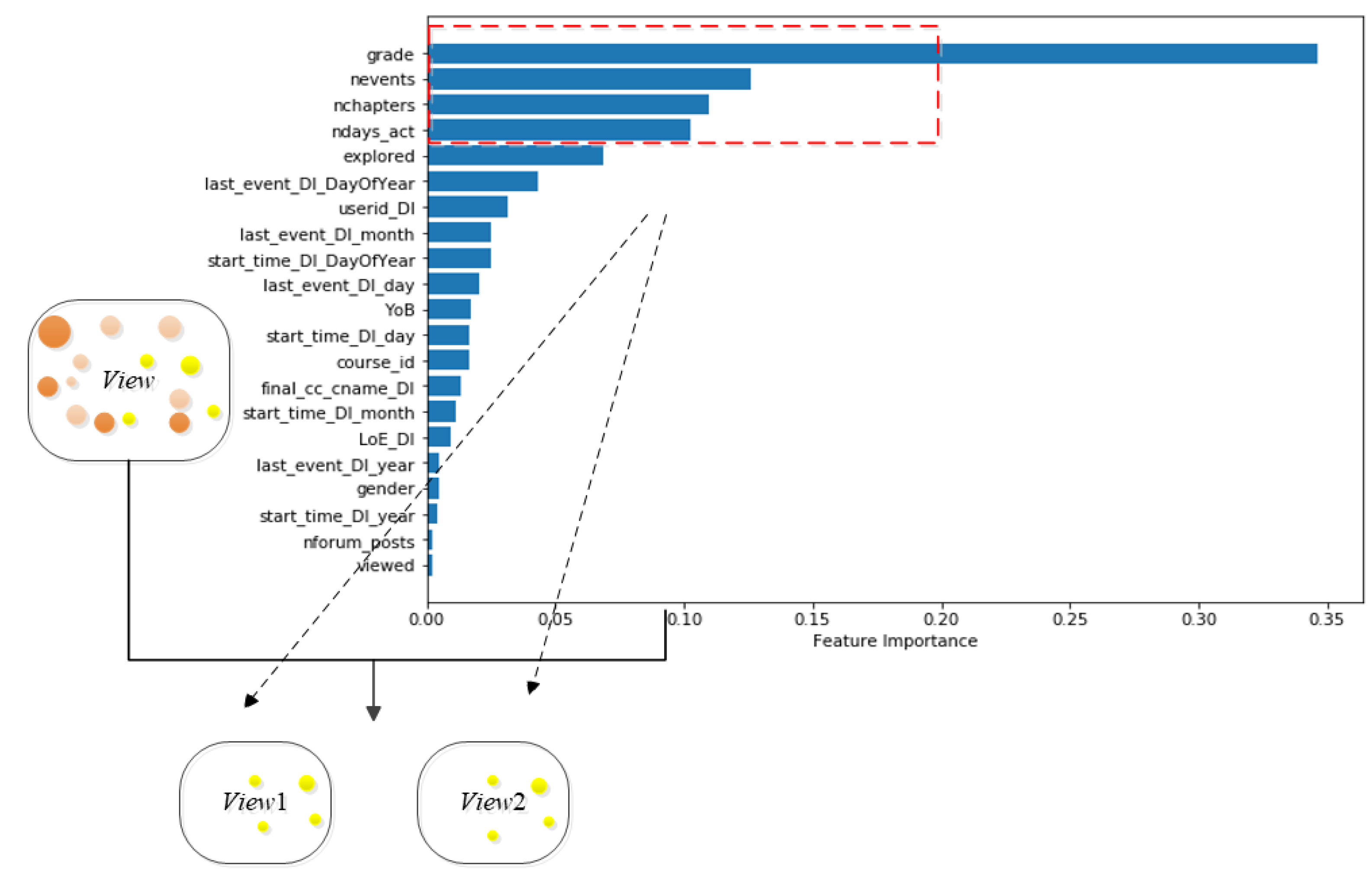
In the process of obtaining independent dual views based on random segmentation, we propose the innovation of semi-decoupled feature co-training. It mainly includes three steps: shared important features selection, remaining features separation, and features combination. First, the importance of the features is calculated and ranked [43,44], and a few important features are selected and added to the dual view together. In addition, we compute the correlation coefficients of the remaining features. Those with larger correlation coefficients are placed in the same view, while those with smaller correlation coefficients are divided into two different views so that the remaining features are retained or separated in two; then, the important features and separated features are combined. With the two views’ acquisition based on semi-decoupled features, on the one hand, it ensures that the strong features continue to play an essential role in the semi-decoupled double view; on the other hand, it minimizes the interference between weak features and weak features in the process of model training and avoids the negative influence caused by attribute conflict between features as much as possible. The major calculations in this process are shown below.

3.2.1. Feature Importance

According to the Gini index and the random forest algorithm, feature importance is calculated and ranked. The smaller the Gini index, the better the feature attributes. The calculation formula is as follows, where D denotes a certain dataset; v and V refer to the value of a feature and the total number of features respectively; p_fx means the proportion of positive cases of feature f_x in the dataset; p_fx′ = 1 − p_fx.

$$Gini\left(View\right)={\displaystyle \sum }_{v=1}^V{\displaystyle \sum }_{f_x\prime \ne f_x} p_{f_x}\times p_{f_x}\prime =1-{\displaystyle \sum }_{v=1}^V p_{f_x}{}^2$$

(1)

$$Gini\left(feature,f_x\right)={\displaystyle \sum }_{v=1}^V\frac{| D^v|}{\left| D \right|}Gini\left(D^v\right)$$

(2)

The concept of shared features is displayed in Figure 2. The orange part of the View shows the important features, and the other two colored parts show the remaining features. The feature importance histogram was used to select the important features, and View1 and View2 both stand for the dual views after sharing the important features.

3.2.2. Correlation Coefficient between Features and Features

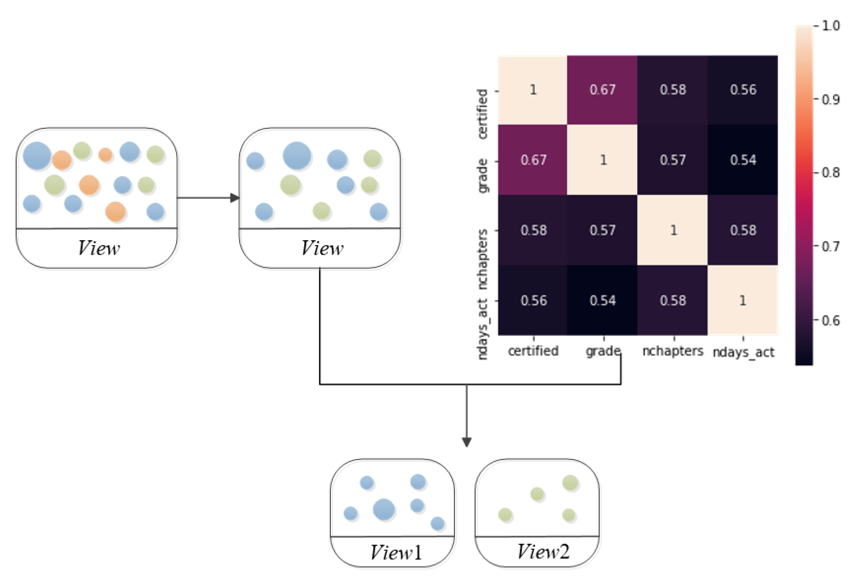
Through calculating the Pearson correlation coefficient and the assistance of a heat map, the remaining features are separated. The process needs to satisfy the following criteria:

• Those with weak feature correlation do not co-exist in the same view;
• Those with strong feature correlation must co-exist in the same view.

By following the above premise, the features are separated one by one or in small batches, and they are added to View1 or View2, accordingly, until the two views have completed the feature selection of the original single view. Then, the final redundant and more independent dual views, View1 and View2, are formed for co-training. The formula is shown below, where f_x and f_y stand for features x and y; σ_fx and σ_fx represent the variance of features x and y; E(f_x) and E(f_y) denote the mean values of features x and y, respectively.

$${\rho }_{f_x, f_y}=\frac{\mathrm{cov}\left(f_x,f_y\right)}{{\sigma }_{f_x}{\sigma }_{f_y}}=\frac{E\left[\left(fx-{\mu }_{fx}\right)\left(fy-{\mu }_{fy}\right)\right]}{{\sigma }_{fx}{\sigma }_{fy}}$$

(3)

The concept of remaining feature separation is presented in Figure 3. The blue part and the green part show the remaining features, and the orange part represents those important features. This figure extracts the correlation coefficients of some features, for example, to draw a heat map. View1 and View2 indicate that the single view View started to separate the remaining features after removing the shared features.

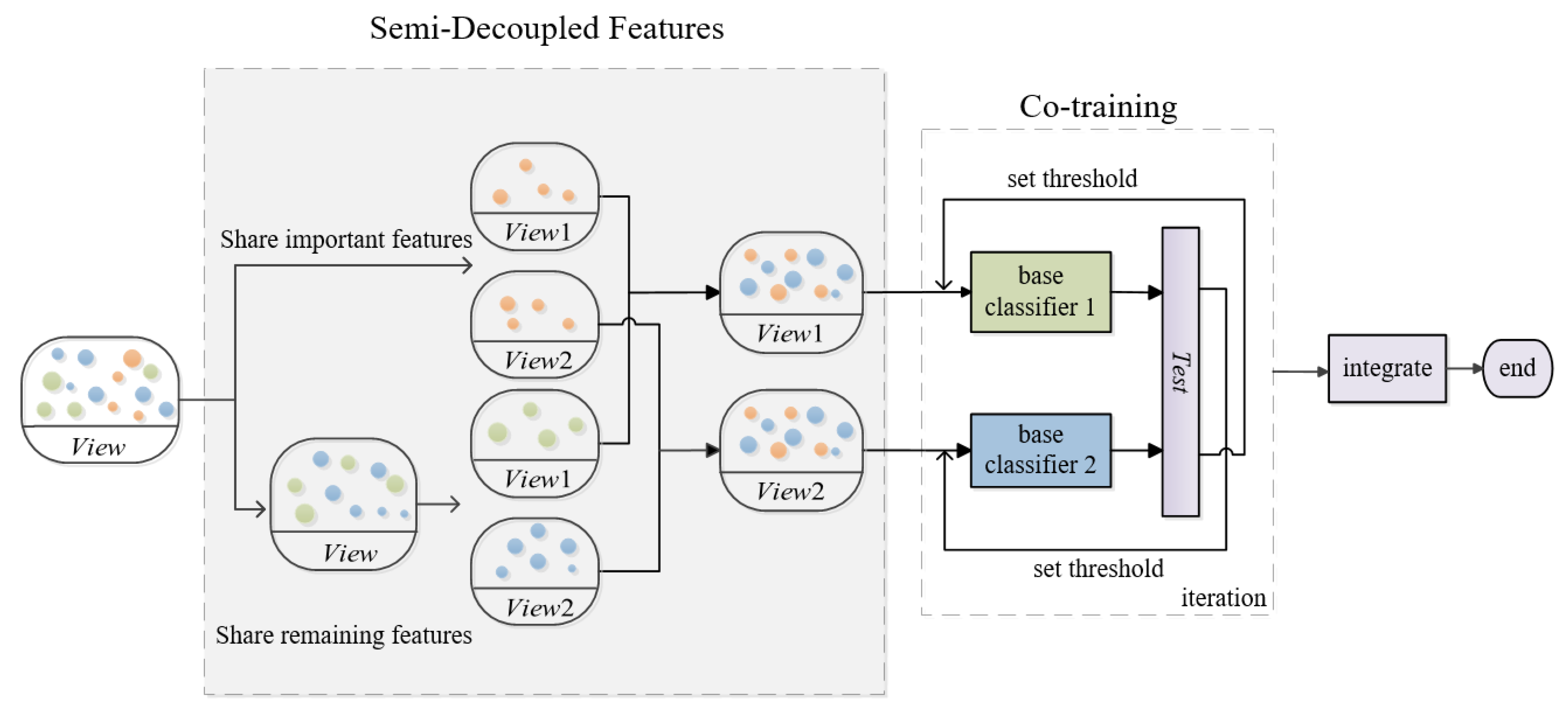
3.3. The Algorithm of Semi-Decoupled Feature Co-Training

The algorithm is presented in Algorithm 1. Here, the samples of the single-view View are labeled, but the samples of Test are not. View1, View2 are empty; ρ_max, ρ_min correspond to maximum threshold, minimum threshold; w₁ and w₂ mean the weights of the predictions from View1 and View2; the whole View includes n features, among them, the set of features F = {f₁, f₂, f₃, …, f_y, …, f_n}, where f_y is the label of the sample.

Algorithm 1: Semi-decoupled feature co-training algorithm.

Input: Single-view View, View1, and View2; ρmax and ρmin; w1 and w2; Test. Output: final_prediction. 1: importance = F.feature_importances_(). //F = F.drop(F.fy) 2: Sort importance. 3: Achieve View’s features sharing. 4: ρfx, ρfy = F.corr(fx, fy). //F includes the feature of fy 5: Divide remaining features. 6: Get View1, View2 with divergence. 7: for iteration = 1, 2, … in iterations: 8:    predict the Test. 9:    if prediction > ρmax 10:     prediction = 1 11:  if prediction < ρmin 12:    prediction = 0 13:  end if 14:    both classifiers no longer change or reach a predetermined 15:  number of iterative rounds. 16: end for

The process of the semi-decoupled feature co-training algorithm is shown in Figure 4. At first, the features are shared; then, those features represented by orange are separated in View1 and View2; in addition, the other features are separated by green into a View1 and the blue into a View2; then, the orange View1 and green View1 and the orange View2 and the blue View2 are combined to realize the construction of a new View1 and new View2; finally, the formal co-training can begin.

4. Results

4.1. Evaluation Metrics

The evaluation metrics used in the experiment included F1, Precision, and Recall.

• F1: The combination of Precision and Recall. Precision and Recall influence each other. If Precision increases then Recall decreases; if Recall increases then Precision decreases; if both need to be balanced, then F1 measure is needed.

$$F1=\frac{2}{\frac{1}{Precision}+\frac{1}{Recall}}$$

(4)

• Precision: The precision rate, which indicates the percent of the positive category samples that were actually positive. TP means that the original case was positive and was predicted to be positive; FP means that the original case was negative but was predicted to be positive.

$$Precision=\frac{TP}{TP+FP}$$

(5)

• Recall: The recall rate, which also refers to as the check-all rate, means the percentage of positive class samples marked as positive. FN represents cases that were originally positive but were predicted to be negative.

$$Recall=\frac{TP}{TP+FN}$$

(6)

4.2. Comparative Experiment

To verify the effectiveness of the innovation model and prevent overfittings in this paper, we introduced K-fold cross-validation to avoid a high variance and bias. First, we set the K-fold cross-validation fold number, K, as 2, 3, and 5. When K = 2, the proportion of the training set and test set was 5:5; when K = 3, the proportion of the training set and test set was 1:2 or 2:1; when K = 5, the proportion of the training set and test set was 2:8 or 8:2. Then, we compared our model with a traditional supervised model, three tree models, and three conventional semi-supervised models. The traditional supervised model used logistic regression (LR) [45]; the integrated tree models used random forest (RF), LightGBM (LGB), and gradient boosting decision tree (GBDT) [46]; the conventional semi-supervised models used self-training [47], co-training, and tri-training. Among them, self-training used GBDT as the base model for screening pseudo-labeled samples; co-training used both LGB and GBDT as the base model to build classifiers with “divergence” [48]; tri-training used GBDT as the base model to vote so as to select the appropriate pseudo-labeled samples.

4.2.1. Test on the edX Dataset

To prove the effectiveness of the algorithm, we used the edX dataset [49], jointly published by Harvard University and MIT, as the sample set for the experiments. This release is composed of de-identified data from the first year (academic year 2013: fall 2012, spring 2013, and summer 2013) of HarvardX courses on the edX platform along with related documentation. There were 338,223 samples in total, and each sample contained 20 features. The specific features and their descriptions [50] are shown in

Table 1. The features table of the edX dataset.

Feature	Feature Description	Feature	Feature Description
course_id	The id of all courses	grade	The grade of a course
userid_DI	The id of all users	start_time_DI	The start time of registration
registered	Whether to register for the course	last_event_DI	The last time of visit
viewed	Whether to access the courseware	nchapters	The learning chapter
explored	Whether to explore the process	ndays_act	The days of interaction
certified	Whether to obtain a certificate	nforum_posts	The number of forum posts
final_cc_cname_	Nationality	nplay_video	The number of videos played
LoE_DI	Academic qualifications	nevents	The number of interactions in the course
YoB	Birthday	roles	The role that MOOC learner played
gender	Gender (male or female)	incomplete_flag	Whether the information is filled in completely

. Among them, certified was the sample label and the criterion for the accuracy. The more similar the result was to the label, the more accurate the algorithm. When certified = 1, this meant that the certificate was obtained, and when certified = 0, this meant that the certificate was not obtained. The number of samples that obtained a certificate or not was 6570 and 331,653 respectively. The website for downloading and detailing data is https://0-doi-org.brum.beds.ac.uk/10.7910/DVN/26147 (accessed on 11 January 2022).

Table 2. Comparison of the results of various models on the edX dataset.

K-Fold Cross-Validation	Division Proportion	Metric	LR	RF	LGB	GBDT	Self-Training	Co-Training	Tri-Training	Ours
K = 2	5:5	F1	0.7345	0.8944	0.9273	0.9754	0.9669	0.9772	0.9781	0.9946
		Precision	0.6562	0.8646	0.8995	0.9658	0.9519	0.9597	0.9712	0.9908
		Recall	0.8339	0.9263	0.9568	0.9851	0.9823	0.9953	0.9851	0.9983
K = 3	1:2	F1	0.7351	0.8859	0.9314	0.9720	0.9686	0.9755	0.9712	0.9940
		Precision	0.6581	0.8550	0.9046	0.9609	0.9574	0.9569	0.9585	0.9898
		Recall	0.8326	0.9191	0.9600	0.9833	0.9801	0.9948	0.9843	0.9982
	2:1	F1	0.7350	0.8927	0.9314	0.9769	0.9684	0.9777	0.9810	0.9941
		Precision	0.6613	0.8708	0.9046	0.9675	0.9574	0.9594	0.9719	0.9893
		Recall	0.8274	0.9158	0.9600	0.9865	0.9798	0.9966	0.9903	0.9990
K = 5	2:8	F1	0.7326	0.8753	0.9198	0.9674	0.9590	0.9727	0.9626	0.9935
		Precision	0.6581	0.8497	0.8912	0.9553	0.9457	0.9536	0.9518	0.9902
		Recall	0.8261	0.9025	0.9504	0.9799	0.9727	0.9927	0.9737	0.9968
	8:2	F1	0.7350	0.8942	0.9322	0.9759	0.9685	0.9771	0.9832	0.9953
		Precision	0.6603	0.8668	0.9028	0.9677	0.9538	0.9584	0.9754	0.9920
		Recall	0.8288	0.9234	0.9636	0.9842	0.9837	0.9965	0.9910	0.9986

illustrates the F1, Precision, and Recall values of different models tested on the edX dataset with the different folds of K-fold cross-validation and different proportions. First, it can be seen that with the increase in the proportion of the training set, when K was the same, the score value for each model also increased, indicating that an increase in training samples can effectively improve the performance of the model. Second, the model metrics can roughly be divided into three intervals. The metrics of models LR and RF were basically below 0.9; the scores of models LGB, GBDT, self-training, co-training, and tri-training were all roughly below 0.99, which reflects a greater performance advantage than LR and RF; while the scores for our model in this paper were all about above 0.99, and the highest scores were achieved in almost every division proportion. These analyses fully illustrate the stability and superiority of the model in this paper. Furthermore, compared with the traditional co-training method, our model had significantly improved scores in each division proportion in which the F1 values increased by 2–3 percentage points, indicating the effectiveness of the semi-decoupled feature method proposed in this paper. In conclusion, this algorithm constructs multiple views with “moderate divergence” based on the perspective of semi-decoupled features, which not only ensures that the important features are shared to play their proper role but also reduces the negative impact caused by feature conflicts.

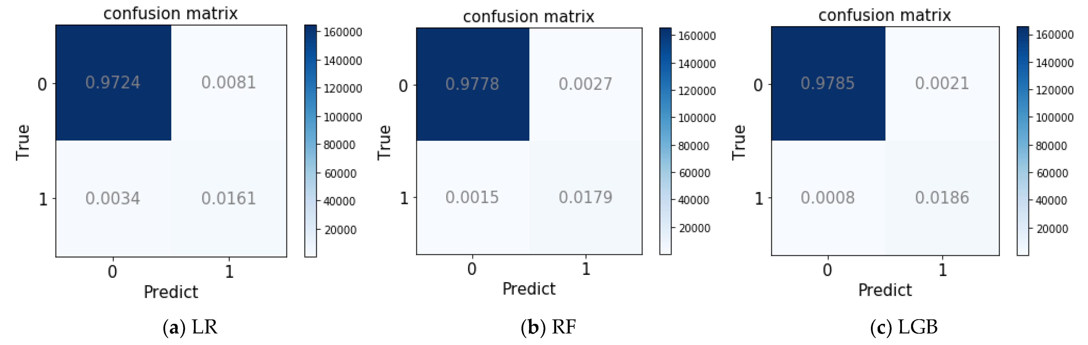
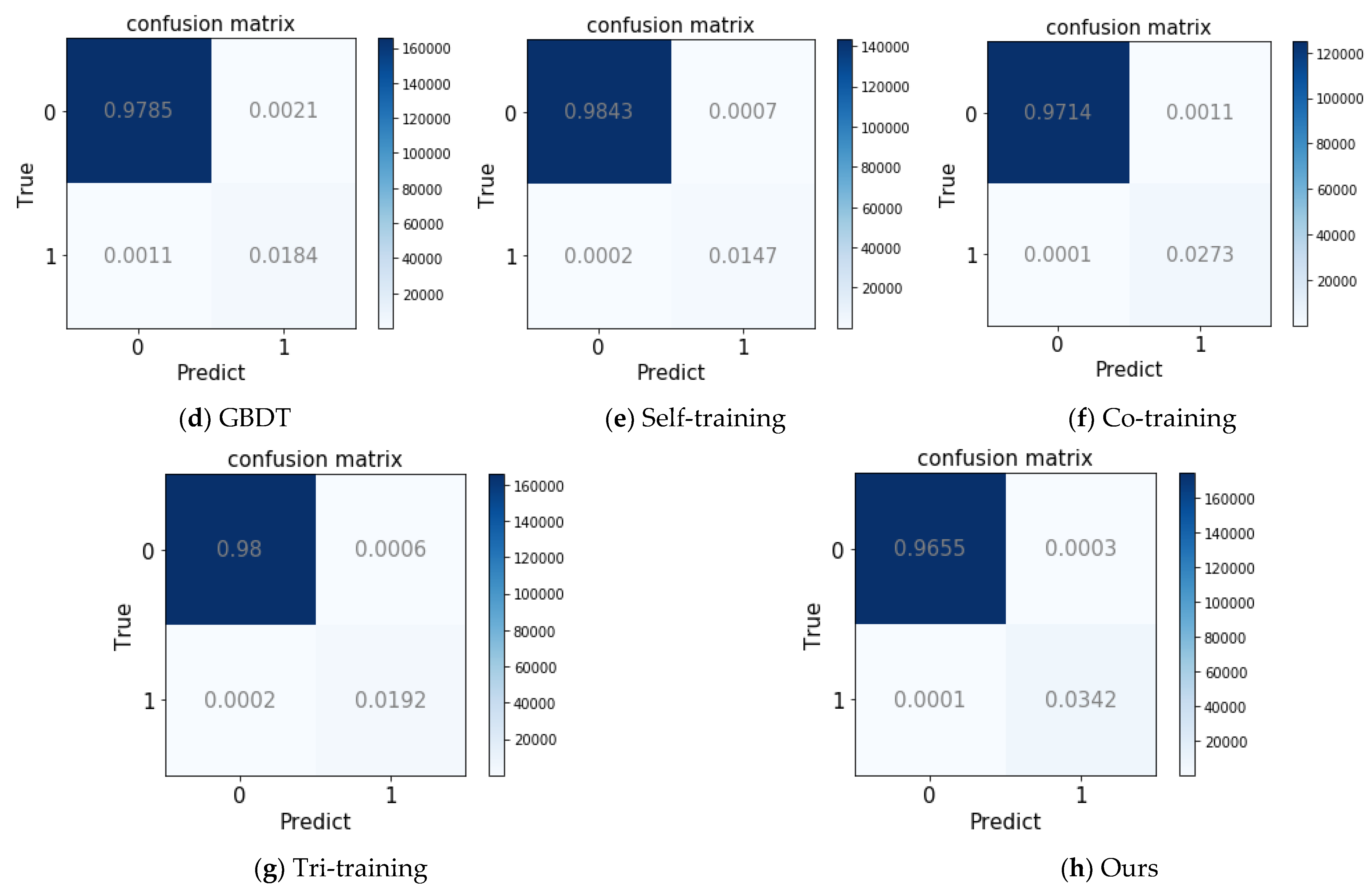
Figure 5 shows the confusion matrix for each model. It was tested on the edX dataset when K = 2 and train:test = 5:5. Figure 5a shows that the LR model obtained the maximum classification error with 0.0115. Figure 5f shows that ours obtained the minimum classification error with 0.0004, 0.0004 higher than the second minimum error produced by tri-training in Figure 5g.

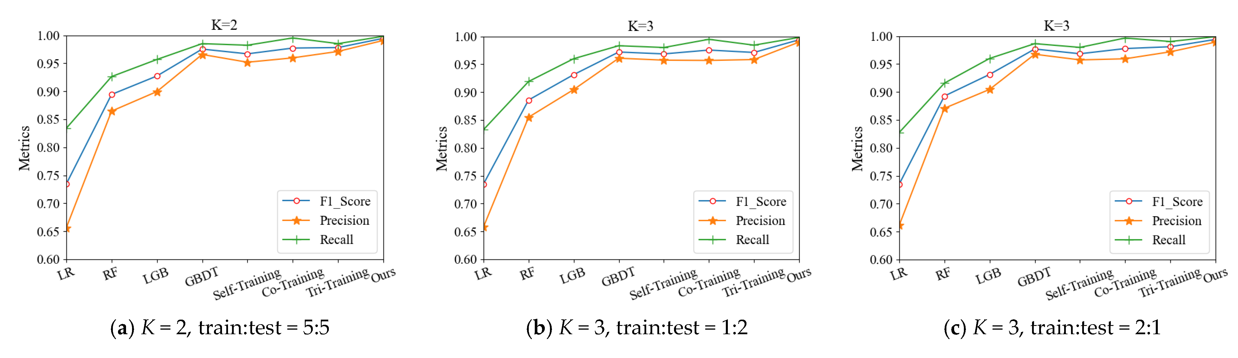
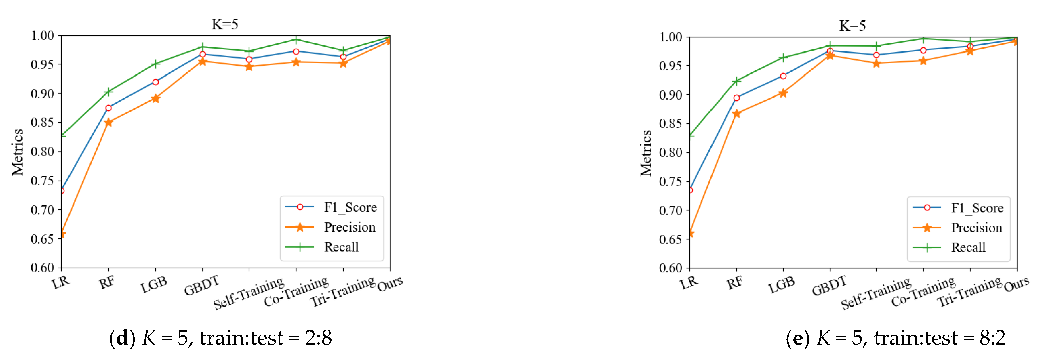
As shown in Figure 6, the evaluation metrics and performance visualization of the different models were carried out. The semi-decoupled feature co-training algorithm presented in this paper all achieved the best results, followed by other semi-supervised models. The LR model showed the worst performance with metrics all lower than 0.85.

4.2.2. Test on the Breast Cancer Wisconsin Dataset

To prove the effectiveness of the model and test its robustness in depth, we also used the Breast Cancer Wisconsin Dataset [51] as the benchmark tested for testing. The dataset can be easily obtained through scikit-learn. There were 569 records in the dataset, with 357 benign and 212 malignant in total. Each sample contained 32 columns with 30 features, and the remaining two were Id and Diagnostic. Every sample was labeled with the benign and malignant results of diagnosis.

Table 3. Comparison of the results of various models on the Breast Cancer Wisconsin Dataset.

K-Fold Cross-Validation	Train:Test	Metric	LR	RF	LGB	GBDT	Self-Training	Co-Training	Tri-Training	Ours
K = 2	5:5	F1	0.9541	0.9721	0.9720	0.9625	0.9760	0.9803	0.9791	0.9859
		Precision	0.9506	0.9721	0.9724	0.9560	0.9674	0.9765	0.9777	0.9748
		Recall	0.9581	0.9721	0.9721	0.9693	0.9847	0.9842	0.9804	0.9974
K = 3	1:2	F1	0.9503	0.9678	0.9644	0.9477	0.9835	0.9831	0.9630	0.9872
		Precision	0.9485	0.9665	0.9599	0.9313	0.9798	0.9755	0.9584	0.9747
		Recall	0.9524	0.9692	0.9692	0.9650	0.9873	0.9908	0.9678	1.0000
	2:1	F1	0.9587	0.9723	0.9767	0.9555	0.9911	0.9909	0.9696	0.9860
		Precision	0.9439	0.9617	0.9597	0.9247	0.9875	0.9847	0.9591	0.9725
		Recall	0.9748	0.9832	0.9944	0.9888	0.9949	0.9974	0.9804	1.0000
K = 5	2:8	F1	0.9432	0.9572	0.9536	0.9288	0.9755	0.9666	0.9578	0.9758
		Precision	0.9344	0.9518	0.9498	0.9072	0.9660	0.9628	0.9531	0.9553
		Recall	0.9524	0.9629	0.9580	0.9517	0.9860	0.9718	0.9629	0.9974
	8:2	F1	0.9574	0.9767	0.9794	0.9622	0.9899	0.9869	0.9767	0.9885
		Precision	0.9491	0.9676	0.9729	0.9422	0.9900	0.9819	0.9678	0.9772
		Recall	0.9667	0.9861	0.9861	0.9833	0.9899	0.9921	0.9861	1.0000

illustrates the F1, Precision, and Recall values of the different models tested on this dataset, using the different folds of K-fold cross-validation and different proportions. First, it can be seen that all models obtained good metrics of approximately 0.95 or more. Moreover, in the supervised model, RF presented the best performance; for the semi-supervised models, both self-training and co-training presented good metrics. However, in most cases, compared with the existing models stated above, our co-training model based on semi-decoupling features still retained the highest metrics when the K and the proportion of the dataset were the same, which proves our model had the best performance once again.

4.3. Iteration Analysis and Discussion

To evaluate the semi-decoupled feature model’s performance at each iteration, on the edX dataset, we used K-fold cross-validation with K = 2, 3, and 5, and then we set the proportion of the training set and test set as 5:5, 1:2, 2:1, 2:8, and 8:2 as well. To explore the iteration’s influence on the model, we conducted four experiments regarding iteration for analysis and discussion.

In

Table 4. Analysis and discussion of the number of iterations.

K-Fold Cross-Validation	Train:Test	Metric	Iteration 1	Iteration 2	Iteration 3	Iteration 4
K = 2	5:5	F1	0.9820	0.9946	0.9902	0.9891
		Precision	0.9729	0.9908	0.9840	0.9815
		Recall	0.9912	0.9983	0.9964	0.9969
K = 3	1:2	F1	0.9804	0.9940	0.9892	0.9871
		Precision	0.9710	0.9898	0.9827	0.9785
		Recall	0.9900	0.9982	0.9957	0.9959
	2:1	F1	0.9825	0.9941	0.9906	0.9891
		Precision	0.9735	0.9893	0.9845	0.9804
		Recall	0.9917	0.9990	0.9967	0.9980
K = 5	2:8	F1	0.9733	0.9935	0.9860	0.9857
		Precision	0.9615	0.9902	0.9797	0.9791
		Recall	0.9853	0.9968	0.9923	0.9925
	8:2	F1	0.9838	0.9953	0.9899	0.9895
		Precision	0.9763	0.9920	0.9825	0.9806
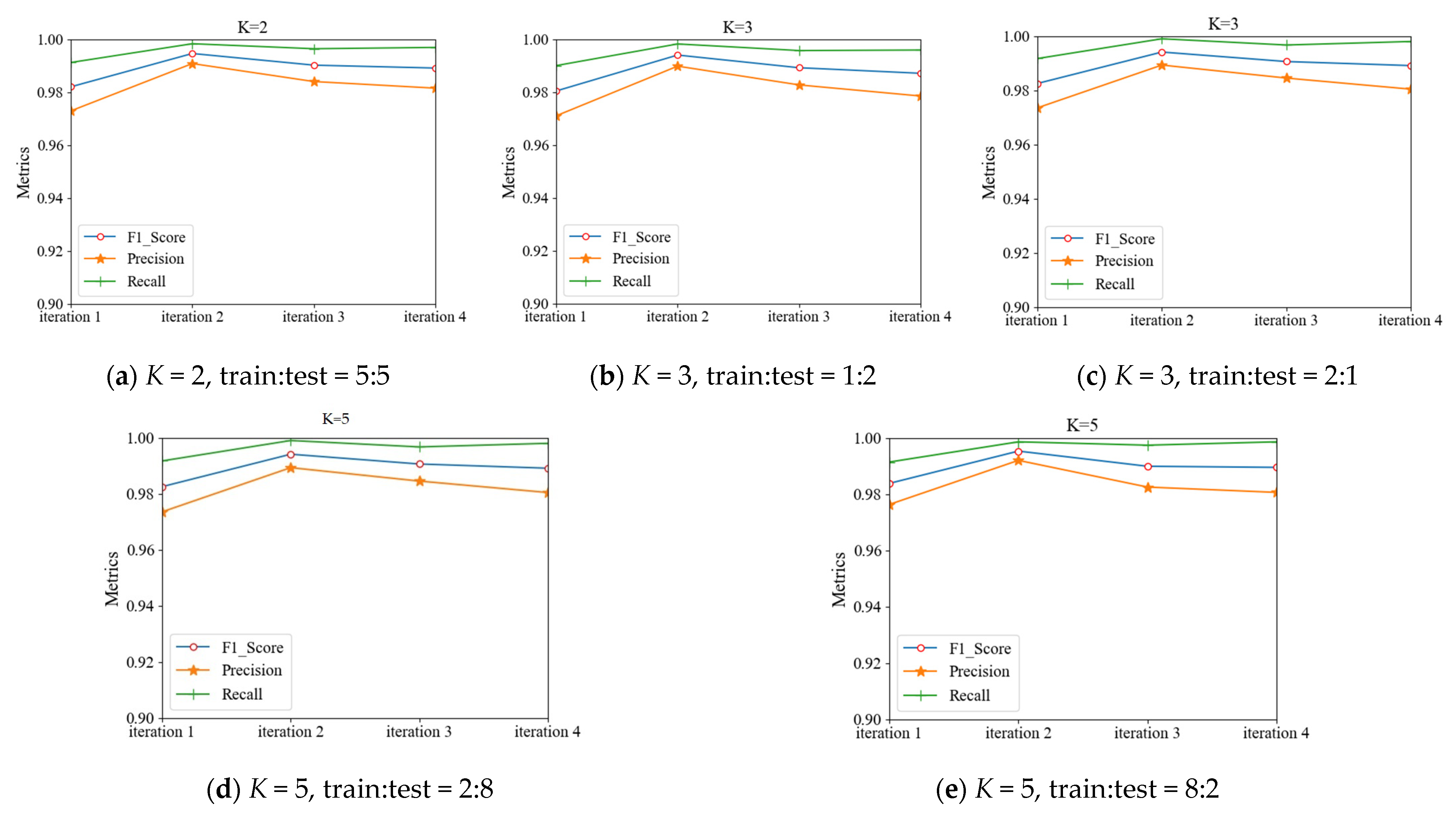
		Recall	0.9914	0.9986	0.9974	0.9986

, the results under different iterations of K-fold cross-validation and proportional division are shown. Top-down, it can be seen that the evaluation metrics increased unstably with the increase in the number of iterations and, overall, the best results were shown at iteration 2. Taking K = 2 and train:test = 5:5 as an example, for iteration 2, F1, Precision, and Recall were 0.9946, 0.9908, and 0.9983, respectively, which were 7–18 thousand points higher than for iteration 1. Then, the overall model improvement effect was gradually limited in iteration 3 and iteration 4. From left to right, when K was the same, with the increase in the samples in the training set, each metric of our model increased, and the highest metric of the model reached 0.9990. On the whole, Table 4 shows that the metrics improved and the performance was optimized with the number of iterations. However, with an increase in the pseudo-label samples, more noise samples will be introduced at the same time. Therefore, the iteration should be stopped after iteration 2, which achieved the best effect in general.

Figure 7 visualizes the effect of our model at different iterations. In Figure 7, we divided the edX dataset into a training set and a testing set with K-fold cross-validation and proportion division. The best effect generated by the iterations was produced and stabilized in iteration 2, and all metrics declined gradually in iteration 3 and iteration 4. In iteration 2, the metrics increased slightly when K = 3, train:test = 2:1 and K = 5, train:test = 8:2, which was due to the greater number of labeled samples and less noise records.

4.4. Hyperparameters

In every experiment, the hyperparameters for the models’ training were all important. Here, we introduce the hyperparameters of some important models tested in experiments: GBDT model, self-training model, co-training model, tri-training model, and co-training model based on semi-decoupling feature. We used GBDT with a learning rate = 0.1, n_estimators = 100, and random_state = 0. In the self-training model, co-training model, tri-training model, and the model proposed in this paper, we used GBDT as the base model and its parameters as the training hyperparameters. In addition, we added LGB as the other base model in co-training with n_estimators = 100, num_leaves = 12, colsample_bytree = 0.5, max_depth = 5, ρ_min < 0.00001, and ρ_max > 0.5. Among them, the hyperparameters ρ_min and ρ_max can be adjusted by the results of the models’ prediction.

5. Discussion

In the comparative experiments of the multiple models, through F1, Precision, Recall, and the confusion matrix, our model showed the better performance and could improve the previous studies by semi-decoupled features. Compared with traditional supervised models, the co-training method based on a semi-decoupling feature model combined the unlabeled and labeled samples fully. Compared with the semi-decoupled models, such as co-training and tri-training, our model made the following main improvements: satisfied the assumptions of standard co-training multiple views; disentangled independent and redundant dual views as much as possible; avoided optimization of the difficulties and conflict problems for important feature attribute features.

The process of semi-decoupled features was mainly based on the importance of features and correlation between features so as to construct “divergent” views. On the one hand, we separated irrelevant features or redundant features based on the Pearson correlation coefficient and a heat map to reduce feature-to-feature interference; on the other hand, we enhanced the influence of important features on the model based on the calculation of feature importance by RF. Since the newly constructed dual views retained the relevant features, the model could achieve significant results. Meanwhile, those important features still continued to play an important role, and features with low correlation coefficients interfered less with each other after view segmentation.

In the process of semi-decoupling features, the importance of features can be calculated and selected not only by using the Gini index but also by combining the ANOVA f-test, mutual information, chi-square test, regression t-test, and variance check, etc., which may offer more reasonable and stable conclusions. The correlation between features can be assessed not only by the Pearson correlation coefficient but also by Spearman, Kendall, etc., in order to realize feature coexistence or separation.

This improved model is certainly applicable to semi-supervised learning of other tabular data, which can be achieved by semi-decoupling the data features into two tables with independence and redundancy. In addition, this work is not only limited to regular data but can be extended into the field of deep learning with non-tabular data.

Overall, this paper proposed a semi-decoupled feature co-training method that solves the current challenge, where the acquisition of multiple views is difficult to achieve. It improves the accuracy of the model, increases the high applicability of standard co-training, and opens up a further development prospect for semi-supervised learning.

6. Conclusions

In this paper, we proposed a co-training algorithm based on semi-decoupled features, which solves the problem of how to obtain fully redundant, conditionally independent dual views. It applied Precision, Recall, F1, and confusion matrix as the evaluation criteria to verify the generalization and learning performance of the training model with the algorithm. Through the experiments, we make the following conclusions.

Different from supervised learning and unsupervised learning, semi-supervised learning can learn on both the massive unlabeled data and limited labeled data at the same time so as to improves the performance in depth. As a popular semi-supervised learning algorithm, co-training has become a research hotspot in the field of machine learning. Co-training requires sufficiently redundant and conditionally independent dual views, which is hard to achieve in real situations. Although many existing improvements generate different learners through different learning algorithms, different data adoptions, etc., they are still unable to meet the requirements of co-training. Thus, we proposed the co-training method based on a semi-decoupling feature algorithm. The innovate algorithm effectively solved the problem of independent view division, according to the two semi-decoupled standards of feature importance and correlation coefficients between features. This created both sufficient and different dual views for standard co-training. The experiments were conducted from three aspects: multiple models, iterations, and hyperparameters.

The contributions of the present study are three-fold. First, we innovated the algorithm in terms of view segmentation, which solved the common problem of massive single views but few multi-views in real scenes. Second, in co-training, there are some algorithms based on view segmentation that exist, but they still suffer from shortcomings with conflicting feature attributes and limitations of irrelevant features. In this study, we can avoid these disadvantages and can make more contributions: disentangling independent and redundant dual views on known single views as much as possible; satisfying the assumptions of standard co-training multiple views; avoiding the problems of conflicting feature attributes and difficulties in optimizing important features; improving the performance of the classifier. Third, the algorithm in this paper is really easy to achieve and effectively solves the problem that multiple views are difficult to see in many practical applications.

Although, the experiments prove that the algorithm in this paper has some improvements in co-training, there are still some limitations for future research to explore. First, with the increase in iterations, the noise samples added to the next training iteration will accumulate step by step and, consequently, its negative effect will become increasingly larger. Second, in a dataset with inadequate features, if the features are still semi-decoupled, the features used for training will be extremely scarce and may cause the results to be very poor. Third, in a dataset with enormous features, if we use feature semi-decoupling to realize feature separation according to feature importance and correlation coefficients, the workload will be very large.

As a summary of the above, the methodology used in this study can be extended to several solid future research directions. This paper did not discuss the problem of noise samples caused by pseudo-label samples. Thus, how to find and deal with these noisy data is a direction that deserves study in depth. In addition, in co-training, how to deal with those noise features, which are not important and have low Pearson correlation coefficients, is another direction. Furthermore, in a dataset with enormous features, with minimal workload, how to apply the idea of feature semi-decoupling is also a direction.

References

- Han, S.; Han, Q. Review of semi-supervised learning research. Comput. Eng. Appl. 2020, 56, 19–27. [Google Scholar]
- Liu, Y.; Zheng, Y.; Jiang, L.; Li, G.; Zhang, W. A survey on pseudo-labeling methods in deep semi-supervised learning. Comput. Sci. Explor. 2022, 15, 1–15. [Google Scholar]
- Saravanan, R.; Sujatha, P. A state of art techniques on machine learning algorithms: A perspective of supervised learning approaches in data classification. In Proceedings of the 2018 Second International Conference on Intelligent Computing and Control Systems (ICICCS), Madurai, India, 14–15 June 2018; pp. 945–949. [Google Scholar]
- Guo, H.; Zhuang, X.; Chen, P. Stochastic deep collocation method based on neural architecture search and transfer learning for heterogeneous porous media. Eng. Comput. 2022. [Google Scholar] [CrossRef]
- Guo, H.; Zhuang, X.; Chen, P. Analysis of three-dimensional potential problems in non-homogeneous media with physics-informed deep collocation method using material transfer learning and sensitivity analysis. Eng. Comput. 2022. [Google Scholar] [CrossRef]
- Ghosh, I.; Chaudhuri, T.D. FEB-stacking and FEB-DNN models for stock trend prediction: A performance analysis for pre and post COVID-19 periods. Decis. Mak. Appl. Manag. Eng. 2021, 4, 51–84. [Google Scholar] [CrossRef]
- Dike, H.U.; Zhou, Y.; Deveerasetty, K.K.; Wu, Q. Unsupervised learning based on artificial neural network: A review. In Proceedings of the 2018 IEEE International Conference on Cyborg and Bionic Systems (CBS), Shenzhen, China, 25–27 October 2018; pp. 322–327. [Google Scholar]
- Li, N.; Shepperd, M.; Guo, Y. A systematic review of unsupervised learning techniques for software defect prediction. Inf. Softw. Technol. 2020, 122, 106287. [Google Scholar] [CrossRef] [Green Version]
- Madiraju, N.S.; Sadat, S.M.; Fisher, D.; Karimabadi, H. Deep temporal clustering: Fully unsupervised learning of time-domain features. arXiv 2018, arXiv:1802.01059. [Google Scholar]
- Halimi, O.; Litany, O.; Rodola, E.; Bronstein, A.; Kimmel, R. Unsupervised learning of dense shape correspondence. In Proceedings of the IEEE/CVF Conference on Computer Vision and Pattern Recognition (CVPR), Long Beach, CA, USA, 15–20 June 2019; pp. 4370–4379. [Google Scholar]
- Yan, K.; Huang, J.; Shen, W. Unsupervised learning for fault detection and diagnosis of air handling units. Energy Build. 2020, 210, 109689. [Google Scholar] [CrossRef]
- Bnou, K.; Hakim, A.; Raghay, S. A wavelet denoising approach based on unsupervised learning model. EURASIP J. Adv. Signal Process. 2020, 36, 1–26. [Google Scholar] [CrossRef]
- Engelen, J.V.; Hoos, H.H. A survey on semi-supervised learning. Mach. Learn. 2020, 109, 373–440. [Google Scholar] [CrossRef] [Green Version]
- Tu, E.; Yang, J. A review of semi-supervised learning theories and recent advances. J. Shanghai Jiaotong Univ. 2018, 52, 1280. [Google Scholar]
- Schmarje, L.; Santarossa, M.; Schroder, S.M.; Koch, R. A survey on semi-, self- and unsupervised learning for image classification. IEEE Access 2021, 9, 82146–82168. [Google Scholar] [CrossRef]
- Park, S.; Lee, J.; Kim, K. Semi-supervised distributed representations of documents for sentiment analysis. Neural Netw. 2019, 119, 139–150. [Google Scholar] [CrossRef]
- Yang, Y.; Bie, R.; Wu, H. Semi-supervised power iteration clustering. Procedia Comput. Sci. 2019, 147, 588–595. [Google Scholar] [CrossRef]
- Ying, Z.; Wang, F.; Zhai, Y.; Wang, W. Semi-supervised generative adversarial network based on self-attention feature fusion for SAR target recognition. J. Signal Process. 2022, 38, 258–267. [Google Scholar]
- Kang, Z.; Peng, C.; Cheng, Q.; Liu, X.; Tian, L. Structured graph learning for clustering and semi-supervised classification. Pattern Recognit. 2021, 110, 107627. [Google Scholar] [CrossRef]
- Wu, J.; Dong, T.; Jiang, P. Protein structural classes prediction by using laplace support vector machine and based on semi-supervised method. Microcomput. Appl. 2020, 36, 4. [Google Scholar]
- Luo, S.; Wang, Z.; Wang, X. Semi-supervised soft sensor on two-subspace co-training model. J. Chem. Eng. 2022, 73, 1270–1279. [Google Scholar]
- Zhang, D.; Chen, H.; Wang, J. Summary of semi-supervised feature selection. Comput. Appl. Res. 2021, 38, 21–329. [Google Scholar]
- Zhai, X.; Oliver, A.; Kolesnikov, A.; Beyer, L. S4l: Self-supervised semi-supervised learning. In Proceedings of the IEEE/CVF International Conference on Computer Vision, Seoul, Korea, 27–28 October 2019; pp. 1476–1485. [Google Scholar]
- Shi, B.; Sun, M.; Kao, C.; Rozgic, V.; Matsoukas, S.; Wang, C. Semi-supervised acoustic event detection based on tri-training. In Proceedings of the IEEE International Conference on Acoustics, Speech and Signal Processing (ICASSP), Brighton, UK, 12–17 May 2019; pp. 750–754. [Google Scholar]
- Sohn, K.; Berthelot, D.; Carlini, N. Fixmatch: Simplifying semi-supervised learning with consistency and confidence. In Proceedings of the Neural Information Processing Systems, Vancouver, BC, Canada, 6–12 December 2020; Volume 33, pp. 596–608. [Google Scholar]
- Wen, Y.; Liu, S.; Miao, Y.; Yi, X.; Liu, C. Survey on Semi-supervised classification of data streams with concept drifts. J. Softw. 2022, 33, 1287–1314. [Google Scholar]
- Li, J.; Xiong, C.; Hai, S. CoMatch: Semi-supervised learning with contrastive graph regularization. In Proceedings of the IEEE/CVF International Conference on Computer Vision (ICCV), Montreal, BC, Canada, 11–17 October 2021; pp. 9475–9484. [Google Scholar]
- Ning, X.; Wang, X.; Xu, S. A review of research on co-training. Concurr. Comput. Pract. Exp. 2021, e6276. [Google Scholar] [CrossRef]
- Xing, Y.; Yu, G.; Domeniconi, C.; Wang, J.; Zhang, Z. Multi-label co-training. In Proceedings of the 27th International Joint Conference on Artificial Intelligence, Stockholm, Sweden, 13–19 July 2018; pp. 2882–2888. [Google Scholar]
- Wang, D.; Lin, Y.; Chen, J. Application of collaborative training algorithm in fault diagnosis of rolling bearing. Comput. Eng. Appl. 2020, 56, 273–278. [Google Scholar]
- Liang, Y.; Liu, Z.; Liu, W. A co-training style semi-supervised artificial neural network modeling and its application in thermal conductivity prediction of polymeric composites filled with BN sheets. Energy AI 2021, 4, 100052. [Google Scholar] [CrossRef]
- Karlos, S.; Kostopoulos, G.; Kotsiantis, S. A soft-voting ensemble based Co-training scheme using static selection for binary classification problems. Algorithms 2020, 13, 26. [Google Scholar] [CrossRef] [Green Version]
- Wang, Y.; Li, T. Improving semi-supervised Co-forest algorithm in evolving data streams. Appl. Intell. 2018, 48, 3248–3262. [Google Scholar] [CrossRef]
- Hou, F.F.; Lei, W.T.; Li, H. Impr-Co-Forest: The improved Co-forest algorithm based on optimized decision tree and dual-confidence estimation method. J. Comput. 2019, 30, 110–122. [Google Scholar]
- Zhang, M.; Zhou, Z. CoTrade: Confident Co-training with data editing. IEEE Press 2011, 41, 1612–1626. [Google Scholar]
- Liu, A.; Xu, N.; Nie, W. Benchmarking a multimodal and multiview and interactive dataset for human action recognition. IEEE Trans. Cybern. 2017, 47, 1781–1794. [Google Scholar] [CrossRef]
- Guo, W.; Yao, J.; Wang, S. Comparison and research progress of multi-view semi-supervised classification algorithms. J. Fuzhou Univ. 2021, 49, 626–637. [Google Scholar]
- Havlíček, V.; Córcoles, A.D.; Temme, K. Supervised learning with quantum-enhanced feature spaces. Nature 2019, 567, 209–212. [Google Scholar] [CrossRef] [Green Version]
- Liu, J.; Wang, G. Pharmacovigilance from social media: An improved random subspace method for identifying adverse drug events. Int. J. Med. Inform. 2018, 117, 33–43. [Google Scholar] [CrossRef] [PubMed]
- Babaei, M.; Roozbahani, A.; Shahdany, S. Risk assessment of agricultural water conveyance and delivery systems by fuzzy fault tree analysis method. Water Resour. Manag. 2018, 32, 4079–4101. [Google Scholar] [CrossRef]
- Jiang, B.; Zhang, Z.; Lin, D.; Tang, J.; Luo, B. Semi-supervised learning with graph learning-convolutional networks. In Proceedings of the IEEE/CVF Conference on Computer Vision and Pattern Recognition (CVPR), Long Beach, CA, USA, 15–20 June 2019; pp. 11313–11320. [Google Scholar]
- Wang, S.; Li, C.; Wang, R.; Liu, Z.; Wang, M.; Tan, H.; Zheng, H. Annotation-efficient deep learning for automatic medical image segmentation. Nat. Commun. 2021, 12, 5915. [Google Scholar] [CrossRef] [PubMed]
- Wang, H.; Zhu, Y.; Xu, W.; Xu, L.; Huang, Y.; Lu, W. Extraction and importance ranking of features for gait recognition. Chin. J. Med. Phys. 2019, 36, 811–817. [Google Scholar]
- Cai, J.; Luo, J.; Wang, S. Feature selection in machine learning: A new perspective. Neurocomputing 2018, 300, 70–79. [Google Scholar] [CrossRef]
- Kirasich, K.; Smith, T.; Sadler, B. Random forest vs logistic regression: Binary classification for heterogeneous datasets. SMU Data Sci. Rev. 2018, 1, 9. [Google Scholar]
- Xia, Z.; Xue, S.; Wu, L. ForeXGBoost: Passenger car sales prediction based on XGBoost. Distrib. Parallel Databases 2020, 38, 713–738. [Google Scholar] [CrossRef]
- Zou, Y.; Yu, Z.; Liu, X.; Kumar, B.V.K.V.; Wang, J. Confidence regularized self-training. In Proceedings of the IEEE/CVF International Conference on Computer Vision (ICCV), Seoul, Korea, 27 October–2 November 2019; pp. 5981–5990. [Google Scholar]
- Lv, J.; Li, T. A summary of semi-supervised self-training methods. J. Chongqing Norm. Univ. 2021, 38, 98–106. [Google Scholar]
- HarvardX Person-Course Academic Year 2013 De-Identified Dataset, Version 3.0. Available online: https://dataverse.harvard.edu/dataset.xhtml?persistentId=doi:10.7910/DVN/26147 (accessed on 11 January 2022).
- Sun, L.; Zhang, Q.; Zheng, Y. Learners’ online learning behavior analysis based on edX open data. Softw. Guide 2020, 19, 190–194. [Google Scholar]
- Street, W.N.; Wolberg, W.H.; Mangasarian, O.L. Nuclear feature extraction for breast tumor diagnosis. In Proceedings of the IS&T/SPIE 1993 International Symposium on Electronic Imaging: Science and Technology, San Jose, CA, USA, 31 January–5 February 1993; Volume 1905, pp. 861–870. Available online: http://archive.ics.uci.edu/ml/datasets/breast+cancer+wisconsin+(diagnostic) (accessed on 1 May 2022).
Figure 1.
The process of co-training.
Figure 2.
The selection of shared features. Orange parts: the important features, which are selected by feature importance; blue and green parts: the remaining features.
Figure 3.
The separation of the remaining features. Orange parts: the important features; blue and green parts: the remaining features, which require to be separated.
Figure 4.
The process of semi-decoupled feature co-training. Orange parts: the important features; blue and green parts: the remaining features.
Figure 5.
The confusion matrix for each model: (a–h) the confusion matrices obtained using the edX dataset with different models when K = 2 and train:test = 5:5.
Figure 6.
The evaluation metrics for each model: (a–e) the metrics obtained on the edX dataset with different models, which were tested under the different K-fold cross-validation and the different proportional divisions. Blue: F1; orange: Precision; green: Recall.
Figure 7.
The iteration metrics of our model: (a–e) the metrics under the K-fold cross-validations and the percentage of divisions, which were tested on the edX dataset with four iterations. Blue: F1; orange: Precision; green: Recall.