Inertial Iterative Self-Adaptive Step Size Extragradient-Like Method for Solving Equilibrium Problems in Real Hilbert Space with Applications


Abstract
:1. Introduction
- ()
- ()
- ()
- for each and satisfying
- ()
- is convex and subdifferentiable on for each
2. Preliminaries
- (i)
- For all and
- (ii)
- if and only if
- (i)
- with
- (ii)
- (i)
- for each exists;
- (ii)
- each weak sequentially limit point of belongs to set C.
3. Main Results
| Algorithm 1 Modified Popov’s subgradient extragradient-like iterative scheme. |
|
- (i)
- Given and
- (ii)
- Computewhere
4. Applications
- ()
- Solution set is non-empty and F is pseudomonotone on C, i.e.,
- ()
- F is L-Lipschitz continuous on C if there exists a positive constants such that
- ()
- for every and satisfying
- (i)
- Choose and a sequence is non-decreasing such that , , and .
- (ii)
- Computewhile
- (i)
- Choose and
- (ii)
- Computewhile
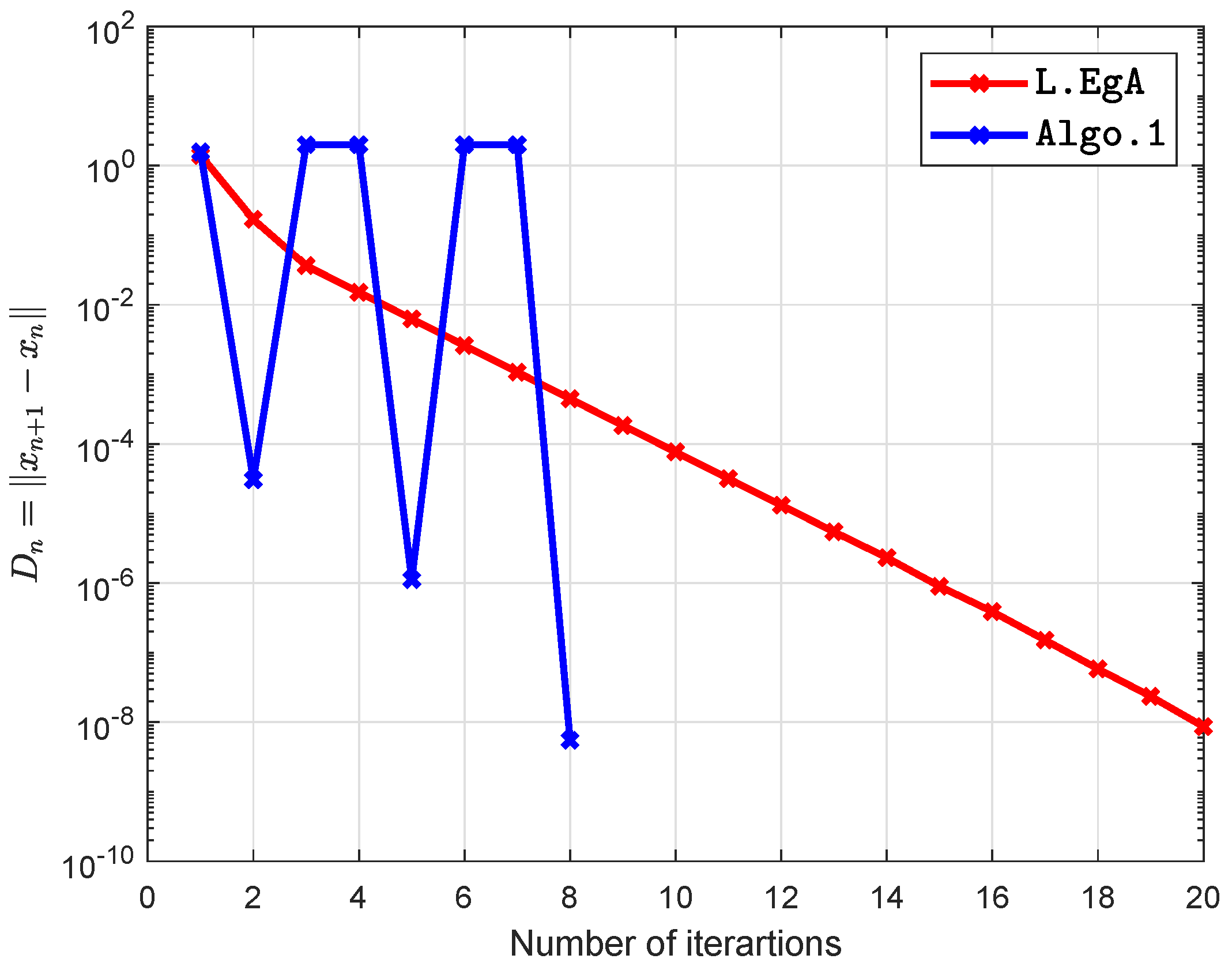
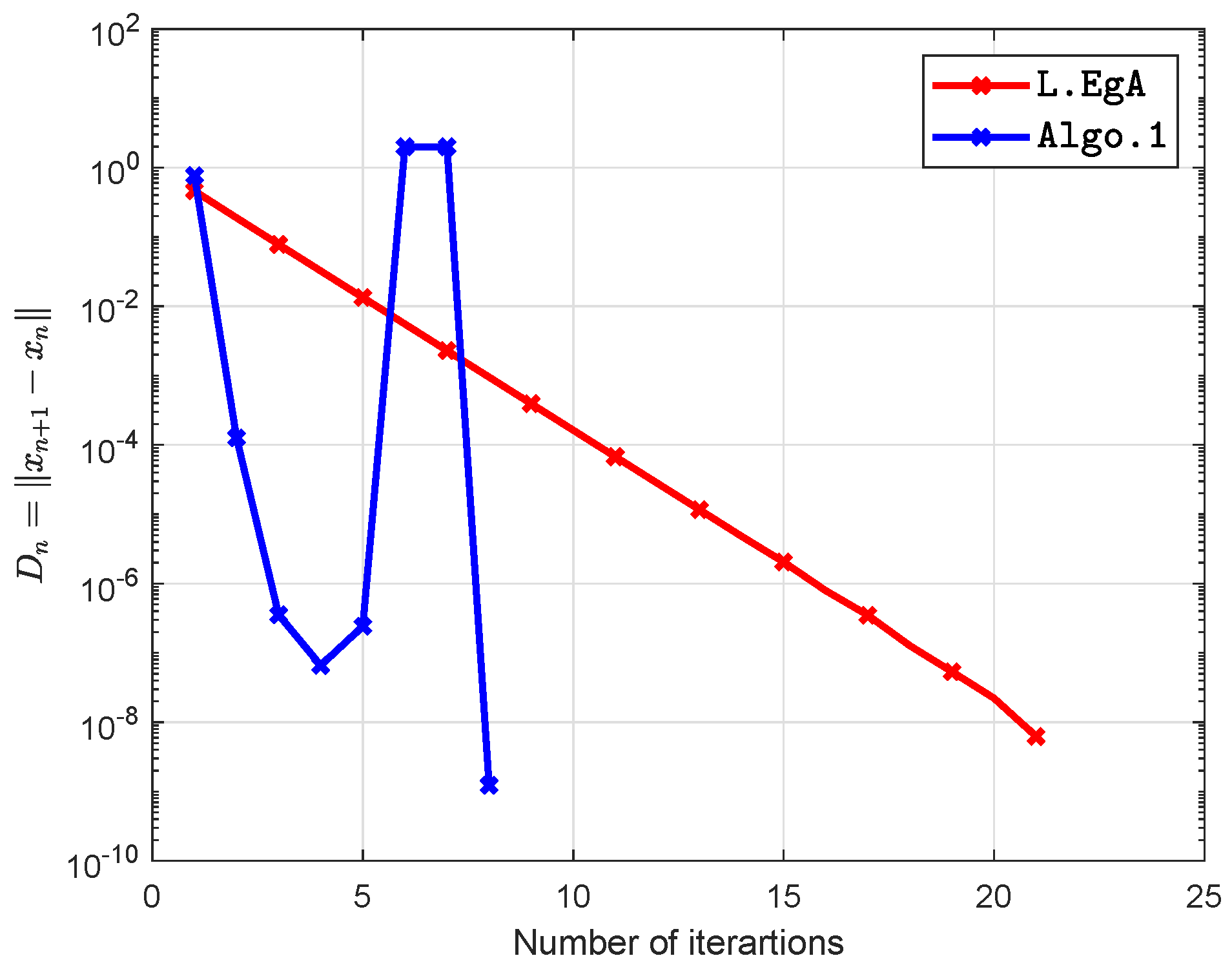
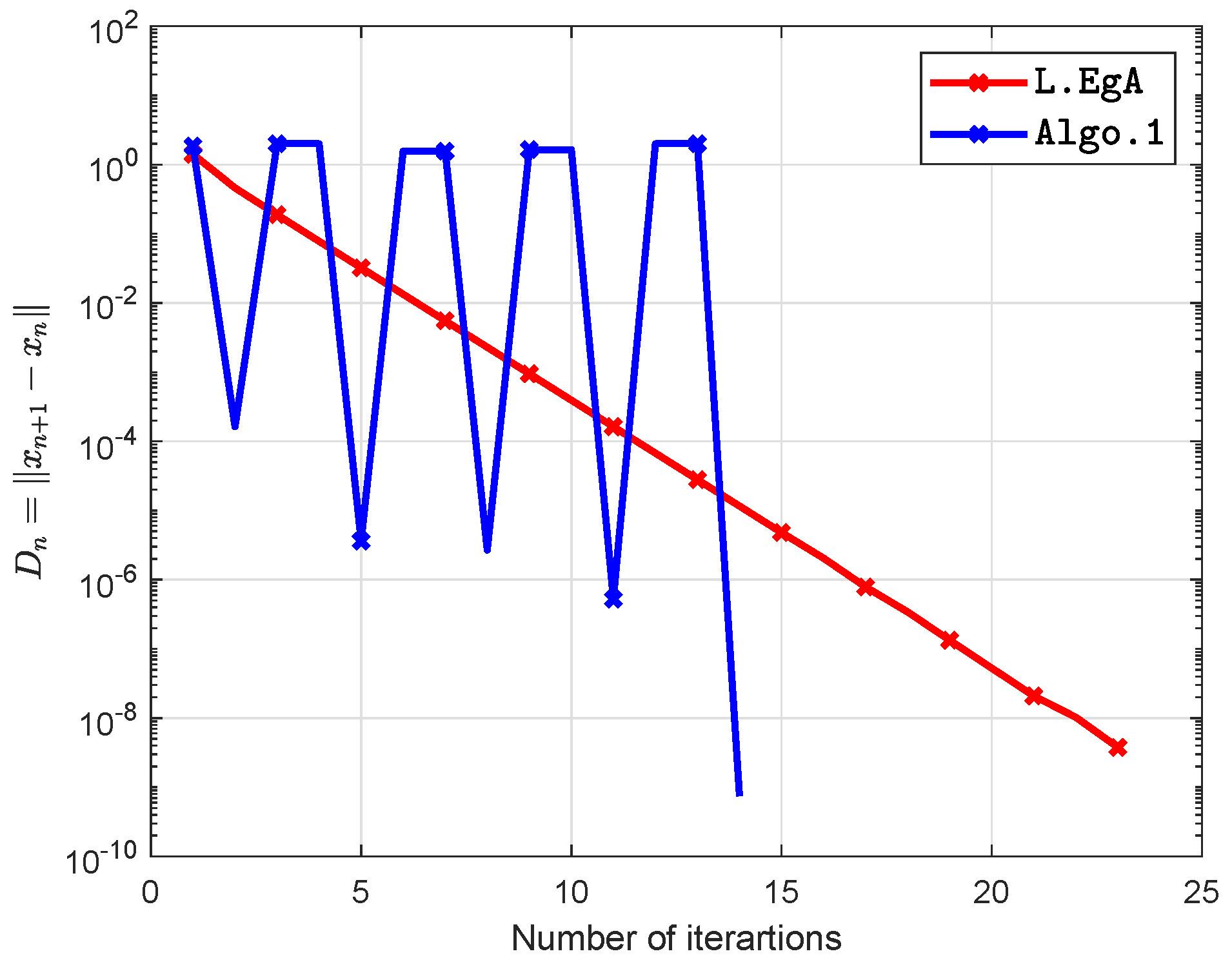
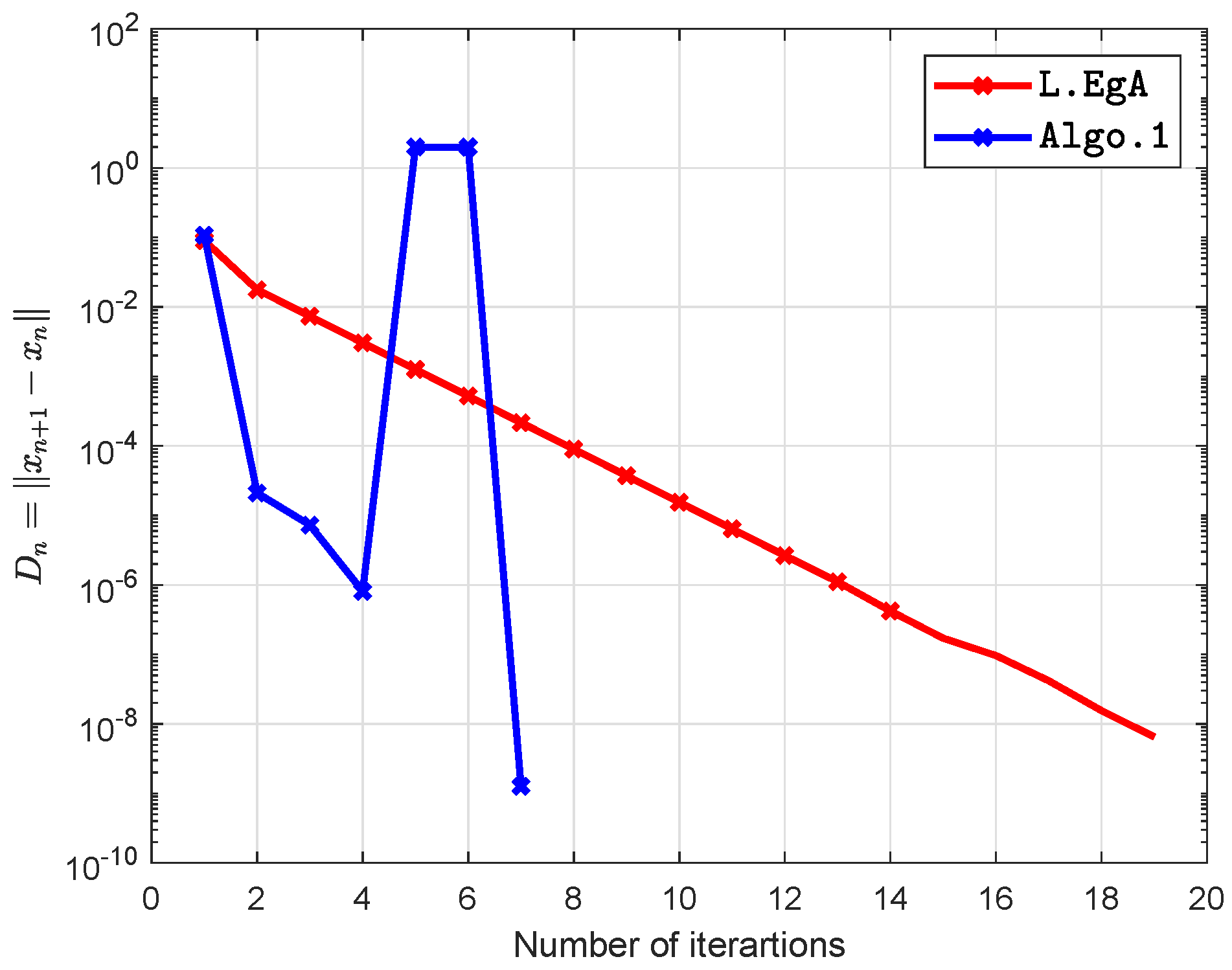
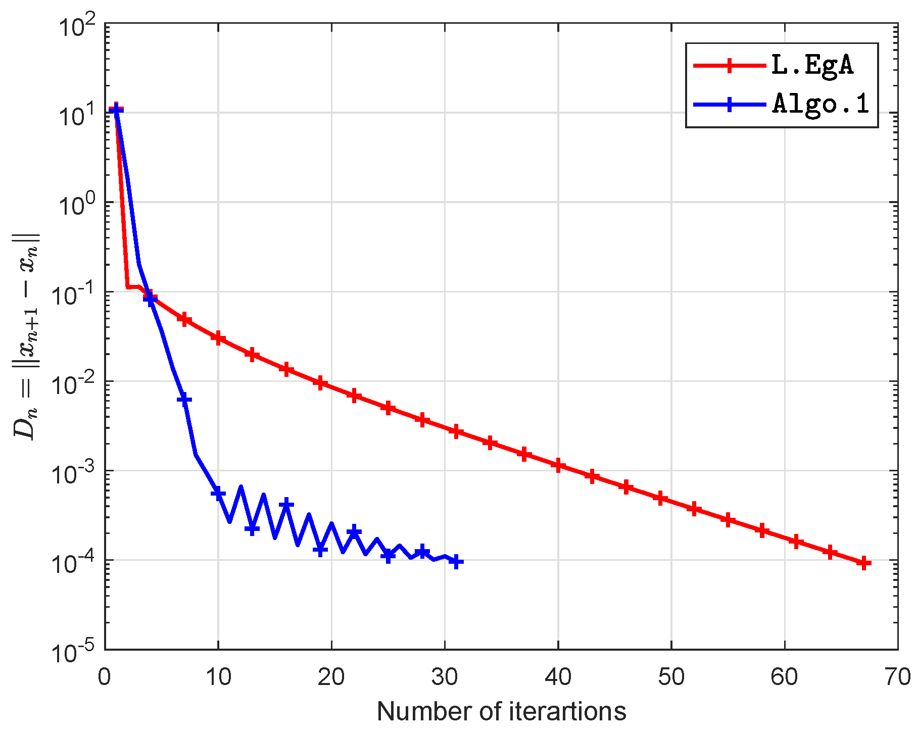
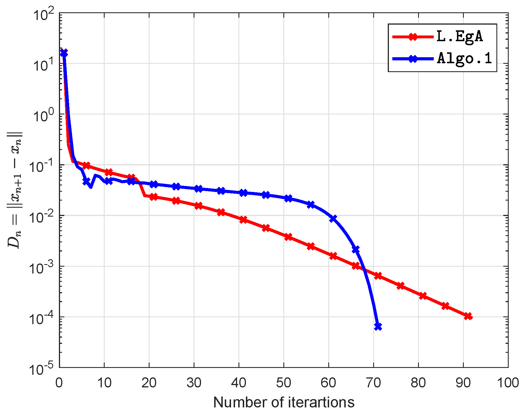
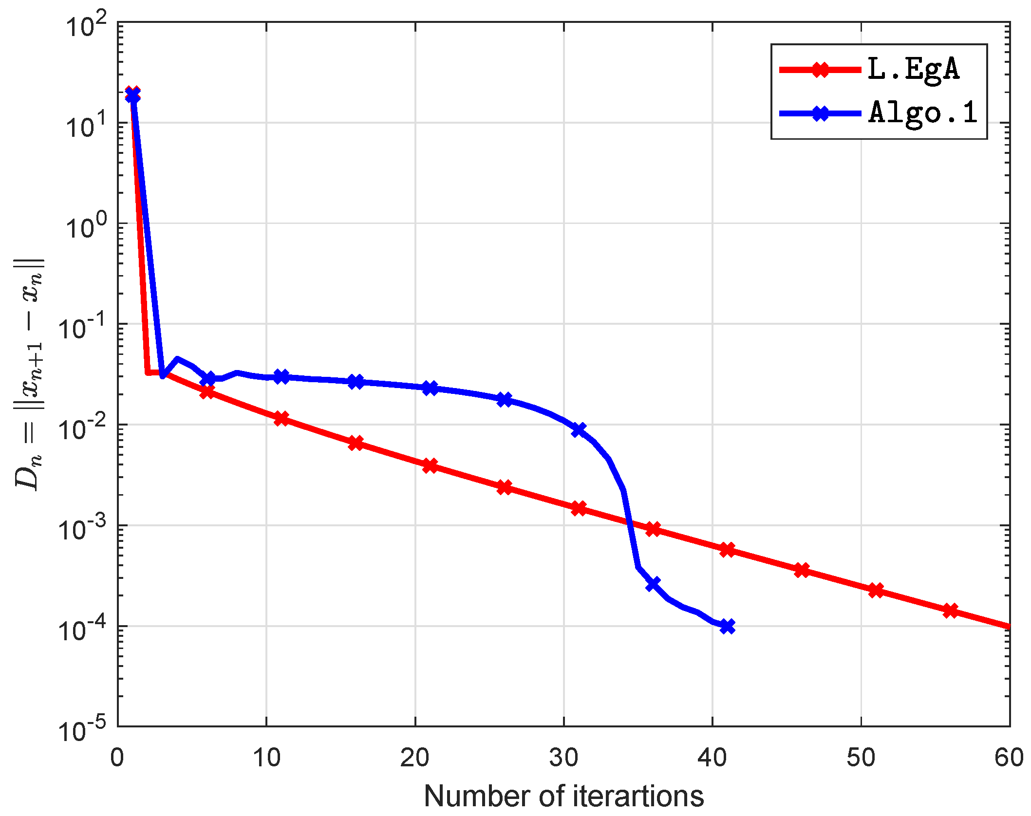
5. Computational Illustration
6. Conclusions
Author Contributions
Funding
Acknowledgments
Conflicts of Interest
References
- Blum, E. From optimization and variational inequalities to equilibrium problems. Math. Stud. 1994, 63, 123–145. [Google Scholar]
- Facchinei, F.; Pang, J.S. Finite-Dimensional Variational Inequalities and Complementarity Problems; Springer Science & Business Media: Berlin/Heidelberg, Germany, 2007. [Google Scholar]
- Konnov, I. Equilibrium Models and Variational Inequalities; Elsevier: Amsterdam, The Netherlands, 2007; Volume 210. [Google Scholar]
- Muu, L.D.; Oettli, W. Convergence of an adaptive penalty scheme for finding constrained equilibria. Nonlinear Anal. Theory Methods Appl. 1992, 18, 1159–1166. [Google Scholar]
- Combettes, P.L.; Hirstoaga, S.A. Equilibrium programming in Hilbert spaces. J. Nonlinear Convex Anal. 2005, 6, 117–136. [Google Scholar]
- Flåm, S.D.; Antipin, A.S. Equilibrium programming using proximal-like algorithms. Math. Program. 1996, 78, 29–41. [Google Scholar]
- Quoc, T.D.; Anh, P.N.; Muu, L.D. Dual extragradient algorithms extended to equilibrium problems. J. Glob. Optim. 2012, 52, 139–159. [Google Scholar]
- Quoc Tran, D.; Le Dung, M.; Nguyen, V.H. Extragradient algorithms extended to equilibrium problems. Optimization 2008, 57, 749–776. [Google Scholar]
- Santos, P.; Scheimberg, S. An inexact subgradient algorithm for equilibrium problems. Comput. Appl. Math. 2011, 30, 91–107. [Google Scholar]
- Takahashi, S.; Takahashi, W. Viscosity approximation methods for equilibrium problems and fixed point problems in Hilbert spaces. J. Math. Anal. Appl. 2007, 331, 506–515. [Google Scholar]
- Ur Rehman, H.; Kumam, P.; Kumam, W.; Shutaywi, M.; Jirakitpuwapat, W. The Inertial Sub-Gradient Extra-Gradient Method for a Class of Pseudo-Monotone Equilibrium Problems. Symmetry 2020, 12, 463. [Google Scholar] [CrossRef] [Green Version]
- Ur Rehman, H.; Kumam, P.; Argyros, I.K.; Alreshidi, N.A.; Kumam, W.; Jirakitpuwapat, W. A Self-Adaptive Extra-Gradient Methods for a Family of Pseudomonotone Equilibrium Programming with Application in Different Classes of Variational Inequality Problems. Symmetry 2020, 12, 523. [Google Scholar] [CrossRef] [Green Version]
- Ur Rehman, H.; Kumam, P.; Shutaywi, M.; Alreshidi, N.A.; Kumam, W. Inertial Optimization Based Two-Step Methods for Solving Equilibrium Problems with Applications in Variational Inequality Problems and Growth Control Equilibrium Models. Energies 2020, 13, 3293. [Google Scholar] [CrossRef]
- Hieu, D.V. New extragradient method for a class of equilibrium problems in Hilbert spaces. Appl. Anal. 2017, 97, 811–824. [Google Scholar] [CrossRef]
- Hammad, H.A.; ur Rehman, H.; De la Sen, M. Advanced Algorithms and Common Solutions to Variational Inequalities. Symmetry 2020, 12, 1198. [Google Scholar] [CrossRef]
- Ur Rehman, H.; Kumam, P.; Cho, Y.J.; Yordsorn, P. Weak convergence of explicit extragradient algorithms for solving equilibirum problems. J. Inequalities Appl. 2019, 2019. [Google Scholar] [CrossRef]
- Ur Rehman, H.; Kumam, P.; Abubakar, A.B.; Cho, Y.J. The extragradient algorithm with inertial effects extended to equilibrium problems. Comput. Appl. Math. 2020, 39. [Google Scholar] [CrossRef]
- Ur Rehman, H.; Kumam, P.; Argyros, I.K.; Deebani, W.; Kumam, W. Inertial Extra-Gradient Method for Solving a Family of Strongly Pseudomonotone Equilibrium Problems in Real Hilbert Spaces with Application in Variational Inequality Problem. Symmetry 2020, 12, 503. [Google Scholar] [CrossRef] [Green Version]
- Koskela, P.; Manojlović, V. Quasi-Nearly Subharmonic Functions and Quasiconformal Mappings. Potential Anal. 2012, 37, 187–196. [Google Scholar] [CrossRef] [Green Version]
- Ur Rehman, H.; Kumam, P.; Argyros, I.K.; Shutaywi, M.; Shah, Z. Optimization Based Methods for Solving the Equilibrium Problems with Applications in Variational Inequality Problems and Solution of Nash Equilibrium Models. Mathematics 2020, 8, 822. [Google Scholar] [CrossRef]
- Rehman, H.U.; Kumam, P.; Dong, Q.L.; Peng, Y.; Deebani, W. A new Popov’s subgradient extragradient method for two classes of equilibrium programming in a real Hilbert space. Optimization 2020, 1–36. [Google Scholar] [CrossRef]
- Yordsorn, P.; Kumam, P.; ur Rehman, H.; Ibrahim, A.H. A Weak Convergence Self-Adaptive Method for Solving Pseudomonotone Equilibrium Problems in a Real Hilbert Space. Mathematics 2020, 8, 1165. [Google Scholar] [CrossRef]
- Todorčević, V. Harmonic Quasiconformal Mappings and Hyperbolic Type Metrics; Springer International Publishing: Berlin/Heidelberg, Germany, 2019. [Google Scholar] [CrossRef]
- Yordsorn, P.; Kumam, P.; Rehman, H.U. Modified two-step extragradient method for solving the pseudomonotone equilibrium programming in a real Hilbert space. Carpathian J. Math. 2020, 36, 313–330. [Google Scholar]
- Lyashko, S.I.; Semenov, V.V. A new two-step proximal algorithm of solving the problem of equilibrium programming. In Optimization and Its Applications in Control and Data Sciences; Springer: Berlin/Heidelberg, Germany, 2016; pp. 315–325. [Google Scholar]
- Polyak, B.T. Some methods of speeding up the convergence of iteration methods. USSR Comput. Math. Math. Phys. 1964, 4, 1–17. [Google Scholar] [CrossRef]
- Bianchi, M.; Schaible, S. Generalized monotone bifunctions and equilibrium problems. J. Optim. Theory Appl. 1996, 90, 31–43. [Google Scholar] [CrossRef]
- Mastroeni, G. On Auxiliary Principle for Equilibrium Problems. In Nonconvex Optimization and Its Applications; Springer: New York, NY, USA, 2003; pp. 289–298. [Google Scholar] [CrossRef]
- Bauschke, H.H.; Combettes, P.L. Convex Analysis and Monotone Operator Theory in Hilbert Spaces; Springer: Berlin/Heidelberg, Germany, 2011; Volume 408. [Google Scholar]
- Tiel, J.V. Convex Analysis; John Wiley: Hoboken, NJ, USA, 1984. [Google Scholar]
- Alvarez, F.; Attouch, H. An inertial proximal method for maximal monotone operators via discretization of a nonlinear oscillator with damping. Set Valued Anal. 2001, 9, 3–11. [Google Scholar] [CrossRef]
- Opial, Z. Weak convergence of the sequence of successive approximations for nonexpansive mappings. Bull. Am. Math. Soc. 1967, 73, 591–597. [Google Scholar] [CrossRef] [Green Version]
- Shehu, Y.; Dong, Q.L.; Jiang, D. Single projection method for pseudo-monotone variational inequality in Hilbert spaces. Optimization 2019, 68, 385–409. [Google Scholar] [CrossRef]


| Unit j | ||||||
|---|---|---|---|---|---|---|
| 1 | 0.04 | 2 | 0 | 2 | 1 | 25 |
| 2 | 0.035 | 1.75 | 0 | 1.75 | 1 | 28.5714 |
| 3 | 0.125 | 1 | 0 | 1 | 1 | 8 |
| 4 | 0.0116 | 3.25 | 0 | 3.25 | 1 | 86.2069 |
| 5 | 0.05 | 3 | 0 | 3 | 1 | 20 |
| 6 | 0.05 | 3 | 0 | 3 | 1 | 20 |
| j | ||
|---|---|---|
| 1 | 0 | 80 |
| 2 | 0 | 80 |
| 3 | 0 | 50 |
| 4 | 0 | 55 |
| 5 | 0 | 30 |
| 6 | 0 | 40 |
| L.EgA | Algo.1 | |||
|---|---|---|---|---|
| TOL | Iter. | time (s) | Iter. | time (s) |
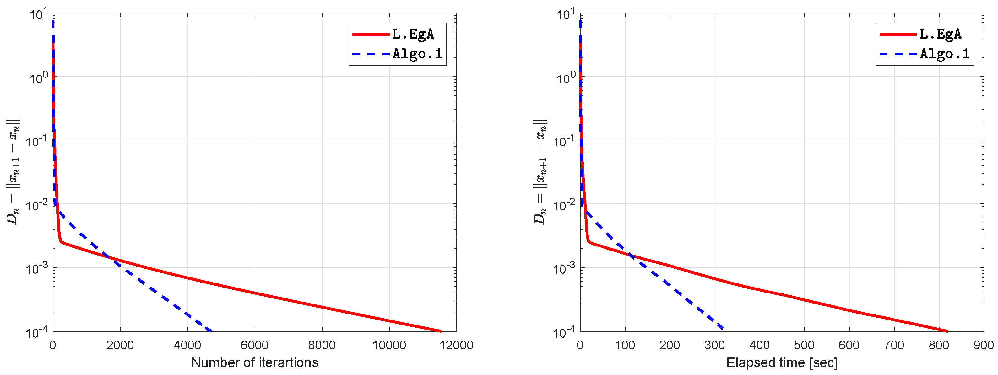
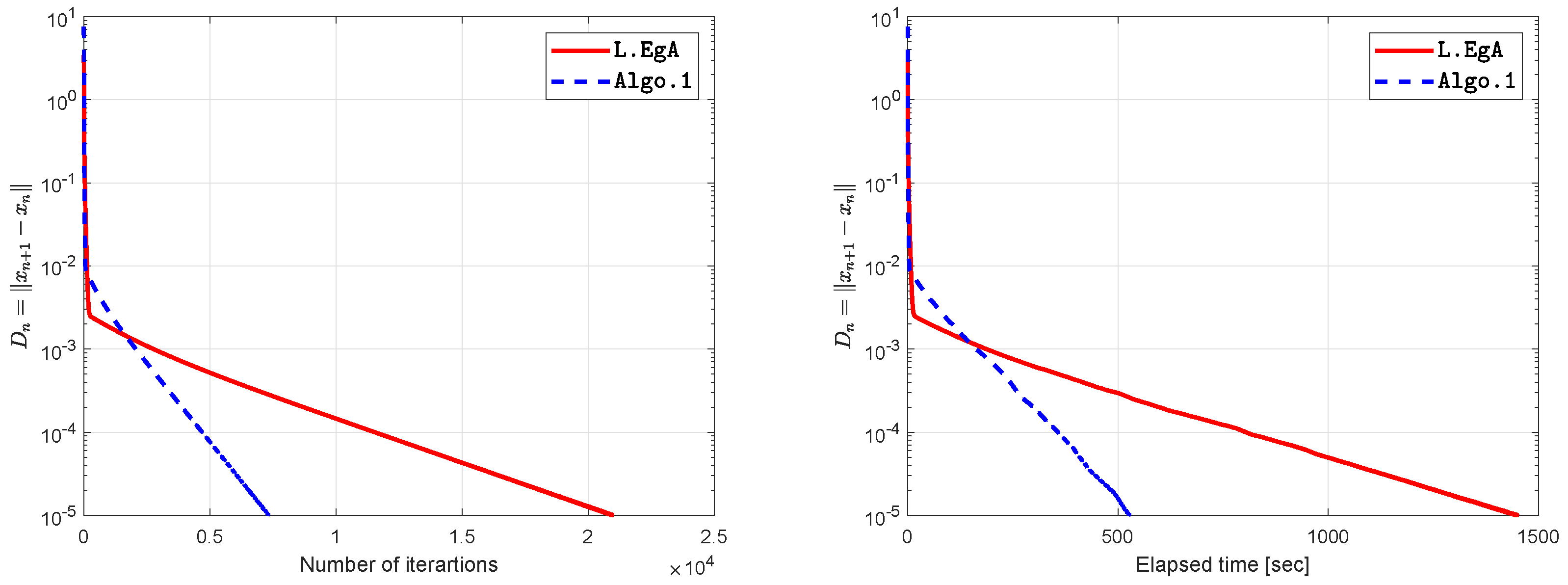
| 0.01 | 125 | 7.3692 | 61 | 3.4055 |
| 0.001 | 2761 | 193.3939 | 2063 | 150.6757 |
| 0.0001 | 11,526 | 818.7184 | 4687 | 324.3571 |
| 0.00001 | 20,946 | 1449.3959 | 7307 | 526.9766 |
| L.EgA | Algo.1 | ||||
|---|---|---|---|---|---|
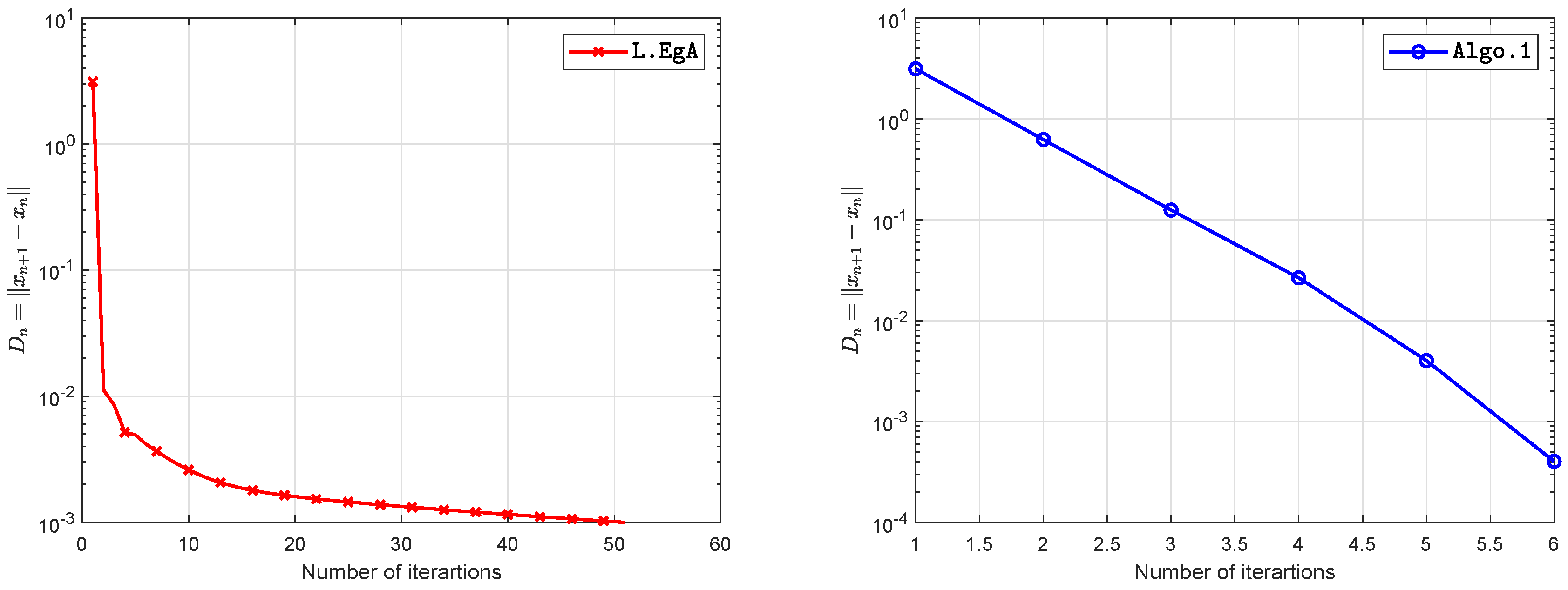
| n | T. Samples | Avg Iter. | Avg time(s) | Avg Iter. | Avg time(s) |
| 5 | 10 | 35 | 0.8066 | 6 | 0.1438 |
| 10 | 10 | 51 | 1.1779 | 6 | 0.1302 |
| 20 | 10 | 84 | 1.7441 | 7 | 0.1801 |
| 40 | 10 | 30 | 0.6859 | 8 | 0.1999 |
| L.EgA | Algo.1 | |||
|---|---|---|---|---|
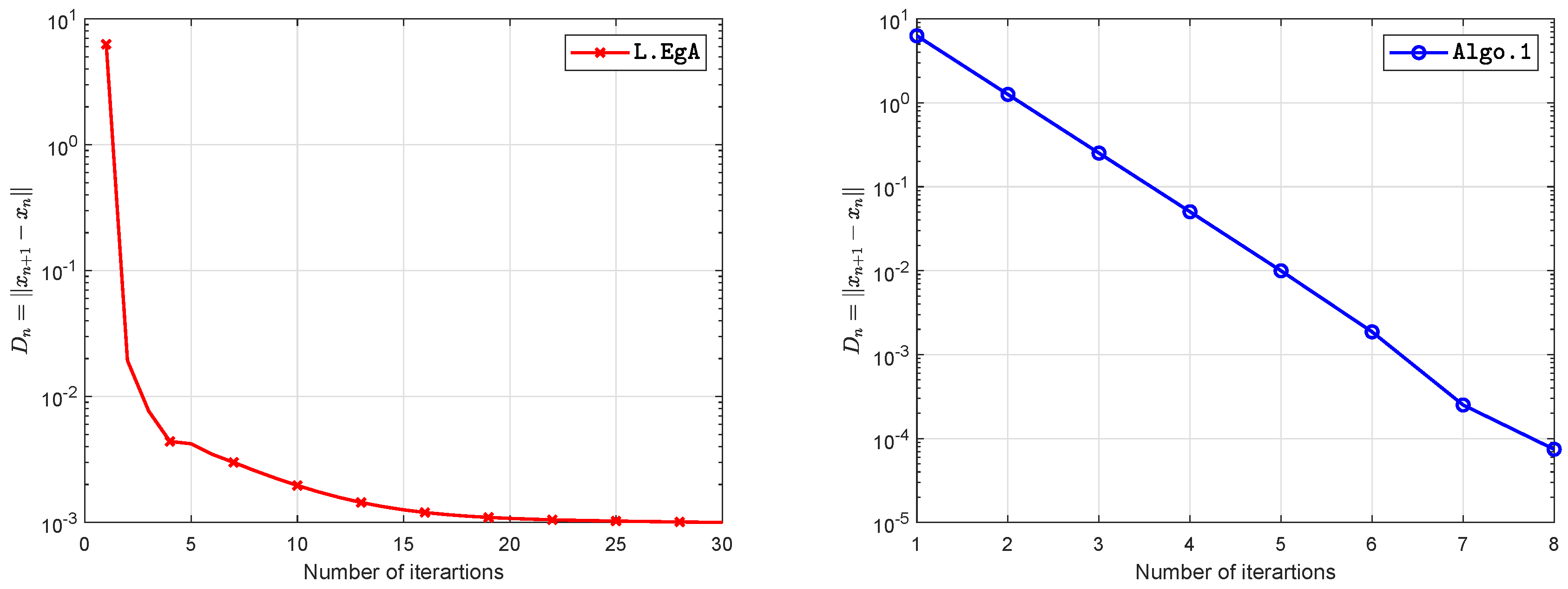
| Iter. | time(s) | Iter. | time(s) | |
| 20 | 0.7506 | 8 | 0.5316 | |
| 21 | 0.7879 | 8 | 0.6484 | |
| 23 | 1.1450 | 14 | 0.9730 | |
| 19 | 0.7254 | 7 | 0.5835 | |
Publisher’s Note: MDPI stays neutral with regard to jurisdictional claims in published maps and institutional affiliations. |
© 2020 by the authors. Licensee MDPI, Basel, Switzerland. This article is an open access article distributed under the terms and conditions of the Creative Commons Attribution (CC BY) license (http://creativecommons.org/licenses/by/4.0/).
Share and Cite
Kumam, W.; Muangchoo, K. Inertial Iterative Self-Adaptive Step Size Extragradient-Like Method for Solving Equilibrium Problems in Real Hilbert Space with Applications. Axioms 2020, 9, 127. https://0-doi-org.brum.beds.ac.uk/10.3390/axioms9040127
Kumam W, Muangchoo K. Inertial Iterative Self-Adaptive Step Size Extragradient-Like Method for Solving Equilibrium Problems in Real Hilbert Space with Applications. Axioms. 2020; 9(4):127. https://0-doi-org.brum.beds.ac.uk/10.3390/axioms9040127
Chicago/Turabian StyleKumam, Wiyada, and Kanikar Muangchoo. 2020. "Inertial Iterative Self-Adaptive Step Size Extragradient-Like Method for Solving Equilibrium Problems in Real Hilbert Space with Applications" Axioms 9, no. 4: 127. https://0-doi-org.brum.beds.ac.uk/10.3390/axioms9040127