
Unified Evaluation Framework for Stochastic Algorithms Applied to Remaining Useful Life Prognosis Problems


1
CIDETEC, Basque Research and Technology Alliance (BRTA), Po. Miramón 196, 20014 Donostia-San Sebastián, Spain
2
Electronics and Computing Department, Mondragon Unibertsitatea, Arrasate, 20500 Gipuzkoa, Spain
*
Author to whom correspondence should be addressed.
Batteries 2021, 7(2), 35; https://0-doi-org.brum.beds.ac.uk/10.3390/batteries7020035
Submission received: 13 April 2021
/
Revised: 11 May 2021
/
Accepted: 20 May 2021
/
Published: 25 May 2021
Abstract
:A unified evaluation framework for stochastic tools is developed in this paper. Firstly, we provide a set of already existing quantitative and qualitative metrics that rate the relevant aspects of the performance of a stochastic prognosis algorithm. Secondly, we provide innovative guidelines to detect and minimize the effect of side aspects that interact on the algorithms’ performance. Those aspects are related with the input uncertainty (the uncertainty on the data and the prior knowledge), the parametrization method and the uncertainty propagation method. The proposed evaluation framework is contextualized on a Lithium-ion battery Remaining Useful Life prognosis problem. As an example, a Particle Filter is evaluated. On this example, two different data sets taken from NCA aged batteries and two semi-empirical aging models available in the literature fed up the Particle Filter under evaluation. The obtained results show that the proposed framework gives enough details to take decisions about the viability of the chosen algorithm.
1. Introduction
Nowadays industry has increased the demand of prognostic solutions to optimize as much as possible the operation efficiency and the return of the investment. RUL prognosis is becoming popular on the design of solution approaches or on decision-make applications. To this end, data mining algorithms are the methods that are having more popularity, and among them, the ones that quantify the uncertainty such as the stochastic algorithms are the most popular ones [1]. However, there are many kinds of available stochastic algorithms and the selection of the optimal algorithm for the desired application becomes non-trivial.
In order to find the optimal algorithm, there are many studies that compare different kinds of stochastic algorithms [2,3] or that present improved algorithms which overcome deficiencies of the original algorithms [4,5]. For that, every author uses different evaluation metrics. The metrics that appear the most on this kind of studies quantify the estimation error, such as the Absolute Error (AE) [6,7,8], the Mean Absolute Error (MAE) [9,10,11], the Mean Squared Error (MSE) [12], the Mean Absolute Percentage Error (MAPE) [13,14,15], the Relative Predicting Error (RPE) [4], the Root Mean Squared Error (RMSE) [5,8,16], the Relative Accuracy (RA) [17,18], the Score [19], the Skill Score (SS) [20], the Bayesian Cramér-Rao Lower Bounds (BCRLB) [21] and their variations considering their mean value [5], maximum value [16], normalized value [22] or their variance [5,23]. In addition to this, metrics that represent the precision on estimating the RUL are also used, such as the probability density function width (PDF width) [24] or the probability on estimating the real RUL [25]. Some other studies also evaluate the timeliness of the algorithms based on more sophisticated metrics such as the Prognosis Horizon (PH) [17,26], α-λ performance [23], the Convergence of the Relative Accuracy (CRA) [18] or the convergence time [27]. There are also studies that evaluate the computational cost of the algorithm in terms of simulation time [23,28] or in terms of amount of required basic operations (FLOPs) [3].
On the latest literature, Wang et al. [12] have evaluated a fractional Brownian motion and Fruit-fly Optimization algorithm with the RE, MSE and RMSE; Rathnapriya et al. [27] have evaluated an improved Unscented Particle Filter calculating the RPE, MSE, RA and the convergence time; Zhao et al. [29] have performed their evaluation with the RE and RMSE; Lyu et al. [30] have calculated the RMSE, the cumulative value of RA and MAPE, and they have displayed the α-λ performance on some graphs to assist the evaluation of the proposed algorithm; Kailong et al. [31] calculated the RMSE and AE; Zhang et al. [32] used the AE (called accuracy index), the PDF width (called precision index) and the RMSE. The inexistence of standardized validation and verification methods for prognostics [33] leads each author to perform the evaluation of those algorithms according to his own chosen metrics and methods. Besides, due to the lack of consensus on the comparison metrics, in many cases, authors only use evaluation metrics that consist of the fitness of the result respect to the prediction data set [8,34], leaving aside some other important characteristics such as the evaluation of the probability distribution of the estimation [35]. Consequently, the direct comparison of the evaluations available in the literature becomes unfeasible.
In addition to this, all these algorithms are tested under certain input constraints (a certain data set and prior knowledge of the system), which influences their performance. In general, each author uses the inputs they have interest in and treat these inputs the way they need to. The fact is that the prognostic algorithm receives as inputs many of the sources of uncertainty on the RUL estimation and these are rarely taken into account on the tested algorithms [36]. This means that when evaluating the algorithm without considering the effect of the uncertainty on the inputs, the algorithm could be penalized or accepted according to how well it fits the prediction respect to the ground truth when accurate prior knowledge and/or accurate data of the future conditions of the component/system is not available.
Besides all this, there are many key design concepts on the stochastic algorithms that change completely their performance and that are not always completely described or taken into account. As a general trend, authors don’t specify the method used on the parameterization of the algorithm [5,21,23,26] even though the chosen parameters have a big influence on the final results [3]. In addition, authors rarely specify the method applied to quantify the uncertainty (the probability distribution) of RUL predictions [37] even though it is known that any prediction would be meaningless for effective decision-making unless uncertainty is carefully accounted for [33].
Motivated by these issues, a unified evaluation framework for stochastic algorithms applied to RUL prognosis problems is presented. This paper provides the base to select the optimal stochastic algorithm, which is not possible today due to the non-agreement on the evaluation framework. In Section 2, the unified evaluation method that contains a set of existing quantitative metrics and a set of qualitative graphs is developed. In Section 3, innovative guidelines on how to design a trial matrix that minimizes the effect of the uncertainty of the inputs are presented. In Section 4, a universal parameterization criterion is introduced. In Section 5, an uncertainty propagation method is presented. Once the framework is completely defined, an example of use is developed in Section 6. Here, the proper definition of the problem is shown (a commonly used stochastic prognosis algorithm applied on a lithium-ion battery RUL prognosis problem). The results are presented and discussed in Section 7. Finally, the Section 8 shows the conclusions.
2. Unified Evaluation Method
The evaluation methods quantify (qualitatively and/or quantitatively) the attributes of a test unit in a certain context with a certain goal. Then, the attributes or features are compared with reference features or with features taken from some other units in the same context.
This paper proposes to measure and quantify the key attributes of a stochastic algorithm by the calculation of some specific set of metrics (quantitative evaluation) along with the display of a set of graphs (qualitative evaluation). The proposal can be used as a standardized language with which technology developers and users can share their findings [33]. The context of the proposed evaluation method on this paper is a RUL prognosis problem (description of the prediction performance) with the goal of developing and implementing robust performance assessment algorithms with desired performance levels as well as implementing the prognostics system within user specifications.
2.1. Quantitative Method
The proposed quantitative method quantifies three key performance attributes on RUL prognosis problems: the correctness, the timeliness and the computational burden. The correctness is the main evaluated performance characteristic on all algorithms. The correctness refers to the accuracy and precision of the predictions on a specific prediction-time-instant. However, the algorithm is likely predicting a more general case under uncertainty. The performance level of the algorithm should be invariant to the prediction-time-instant. Therefore, timeliness is also evaluated. The timeliness refers to the time aspects related to accurate predictions. Additionally, the algorithms are often rejected due to final user requirements. The prognosis algorithm needs to meet the final user requirements. Therefore, the computational burden is also evaluated. To cover all these aspects, we present three set of unified evaluation metrics (Table 1, Table 2 and Table 3).
In addition to these three key performance attributes, there is another key performance attribute, which is not considered in the proposed quantitative method: the confidence. The confidence refers to the level of trust a prediction method’s output can have [33]. The reason why the confidence quantification has been discarded on the proposed quantitative method is that the trust on the output has a higher relationship with the trust on the data and the prior knowledge of the system (inputs) rather than the algorithm itself [25]. The confidence remains almost the same when using the same inputs.
2.1.1. Correctness
When searching for an optimal something, the correctness is what we all think about. Correctness refers to the accuracy and precision of the predicted distributions. The metrics that evaluate the correctness measure the deviation of a prediction output from ground truth and the spread of the distribution at any given time instant that may be of interest to a particular application [33]. For this aim, the proposed metrics to measure the correctness of the obtained output with respect to its desired specification in terms of accuracy are the Root Mean Squared Error (RMSE) of the prediction [5], the Relative Accuracy (RA) of the RUL value [17] and the probability of predicting the ground truth [25]; and in terms of precision is the probability distribution width [24] (Table 1).
The RMSE is one of the most used metrics in evaluation and comparison studies [5,8,38]. In this paper, the prediction RMSE is evaluated as an accuracy indicator (Equation (1)). This metric shows the average difference between ground truth data () and predictions (), quantifying the accuracy on the tracking of the system’s behavior (the trend under the noise). The RMSE is useful to show if there is something off on the tracking of the system’s behavior (accurate predictions usually have low prediction errors), and consequently, on the prediction accuracy of the algorithm. However, the RMSE is also a metric that quantifies the noise of the data respect to the model. Therefore, the accuracy evaluation should not be just based on this metric (the noise on the data set is also affecting the value of this metric).
Therefore, in order to have more information about the accuracy of the prediction algorithm, another metric is proposed: The Relative Accuracy (RA). This metric quantifies the accuracy on predicting the most probable value of the desired events (the end-of-life event). This metric is calculated by Equation (2). The range of values for RA is [−∞,1], where the perfect score is 1 [33].
To complete the accuracy evaluation, the accuracy of the predicted distribution is also quantified. This paper proposes to calculate the probability of predicting the real RUL (), see Equation (3). The probability value is taken from the normalized probability distribution of the predicted RUL. Thanks to this metric, we can also determine if the uncertainty has been underestimated. When the probability of predicting the real RUL is near 0, the uncertainty can be considered underestimated.
Once quantified properly the accuracy of the algorithm, the precision (the spread of the predicted distribution) needs to be addressed. For this, this paper proposes to use the relative probability distribution width (PDF width () [24] or confidence interval [17] shown in Equation (4).
This fourth metric quantifies the relative number of time-instants that are in between the time-instants that delimit a certain central mass probability of the estimated RUL probability distribution.
2.1.2. Timeliness
Timeliness refers to the time aspects related to availability and usability of predictions. The metrics that evaluates this attribute measure how quickly a prediction algorithm produces its outputs, in comparison to the effects that it is mitigating [33]. For this aim, the proposed metrics to measure the timeliness are the Prognosis Horizon (PH) and the Convergence of the Relative Accuracy (CRA) (Table 2).
The PH defines the first time when the prediction satisfies a certain criterion (generally defined by a predefined β threshold, Equation (5)) and uses this time to calculate the period between this event and the event that wants to be predicted (end of live (EOL) event). Thanks to this, the availability aspect of the timeliness attribute is put under evaluation: the greater the PH is, the better the timeliness performance of the algorithm is (faster availability). To standardize this metric, the relative of this metric is proposed in this paper, see Equation (6).
where is the probability mass of the prediction PDF within the α bounds that are given by and .
Thanks to the PH, the most important aspect of timeliness (the availability of predictions) is properly described. However, another aspect of the timeliness is found to be interesting when evaluating and comparing prognostic algorithms: the improvement rate of accuracy and precision metrics with time (the convergence). CRA measures how quickly the relative error on the predictions is reduced. For that, the centroid of the area under the curve for the RA is calculated in the same way as in [18], see Equations (7) and (9).
2.1.3. Computational Performance
Computational performance quantification is required to meet the resource constrains of user application [33]. For this aim, the proposed metric to measure the computational performance is the count of floating-point operations (FLOP) (Table 3). This metric represents the number of numerical operations (both basic and complex mathematical operations translated into basic numerical operations) that the algorithm has on its code. Further details on how to calculate this metric can be found in [3].
2.2. Qualitative Method
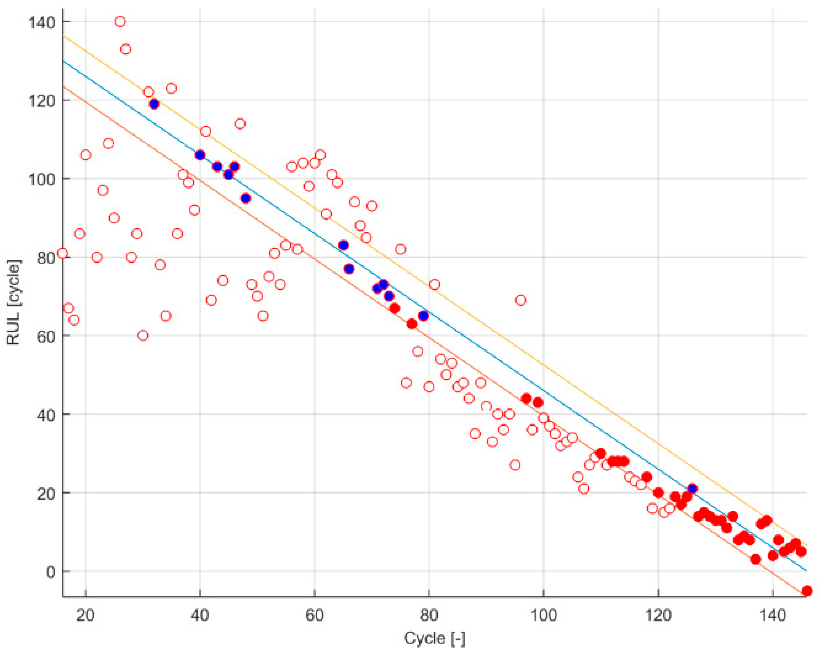
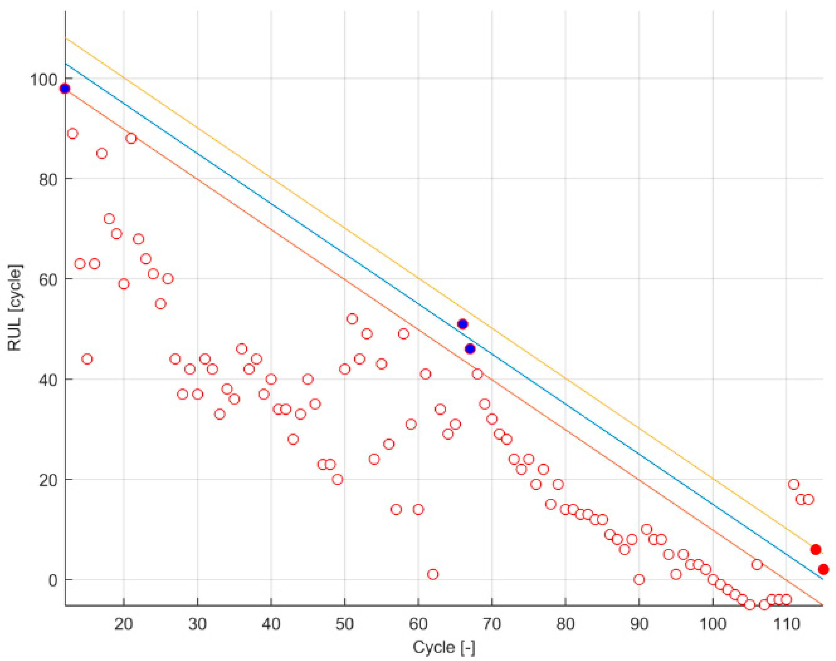
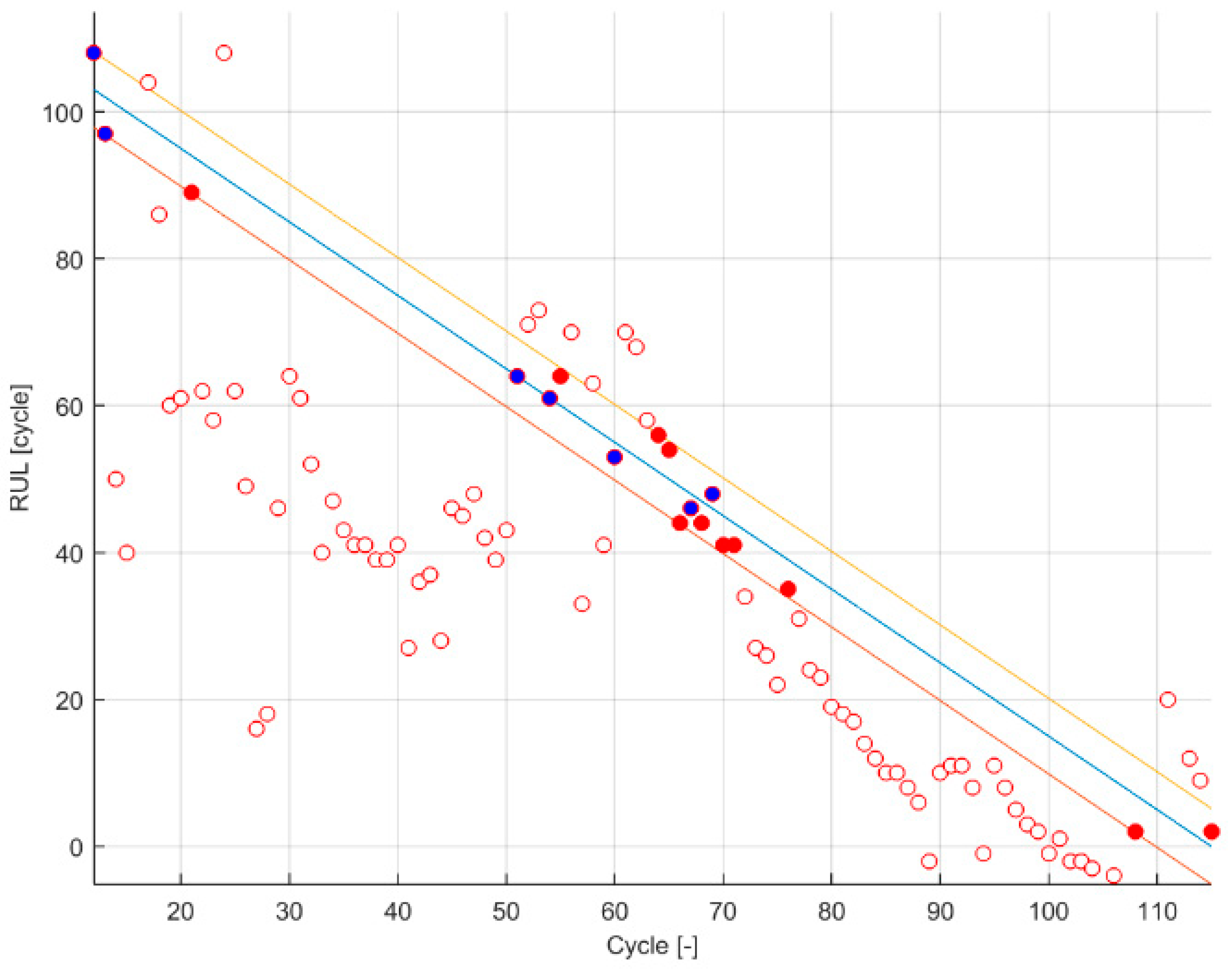
The proposed qualitative method focuses on describing the correctness and timeliness attributes of the prognosis algorithm by a more visual way. For this, a figure that combines the α-λ accuracy [18] and the Prognosis Horizon boundary fulfilment is displayed (Figure 1). This figure can represent both attributes in a synthesized manner and give enough clues when discussing the obtained metrics. It is a modified version of the designed schematic representation of the RA in [18].
In case the discussion needs extra information, a second graphical aid is proposed: the graphical representation of the estimations done by the algorithm for a specific trial at a specific evaluation time (called trial-instant figure in this paper) [25]. This figure shows every detail of the performance of the algorithm at a concrete prediction-time-instant. However, the lack of synthesis on this representation leads us only to propose the use of this graphical aid when there is a mayor doubt on the understanding of the metrics. This figure is the same figure used by some other authors [24,39] when evaluating their prognosis algorithms.
2.2.1. PH and α-λ Accuracy
The PH is already defined as a metric itself, which quantifies the timeliness of the prediction algorithm. However, the illustration of PH boundary fulfilment gives information of the correctness of the prediction algorithm as well. The fulfilment of the PH boundary determines that a β mass of the estimated probability distribution is inside the defined precision boundaries and (Equation (5)).
As for the α-λ accuracy boundary fulfilment, the precision boundaries that delimit the acceptable β mass of the estimated probability distribution are and (Equation (10)) [18].
where is the probability mass of the prediction PDF within the α bounds that are given by and .
Taking advantage that the output of these two metrics is binary, a color code on the PH and α − λ accuracy figure is set (empty circles when both at 0, blue circles when both at 1 and red circles when PH at 1 and α − λ accuracy at 0).
2.2.2. Trial-Instant Figure
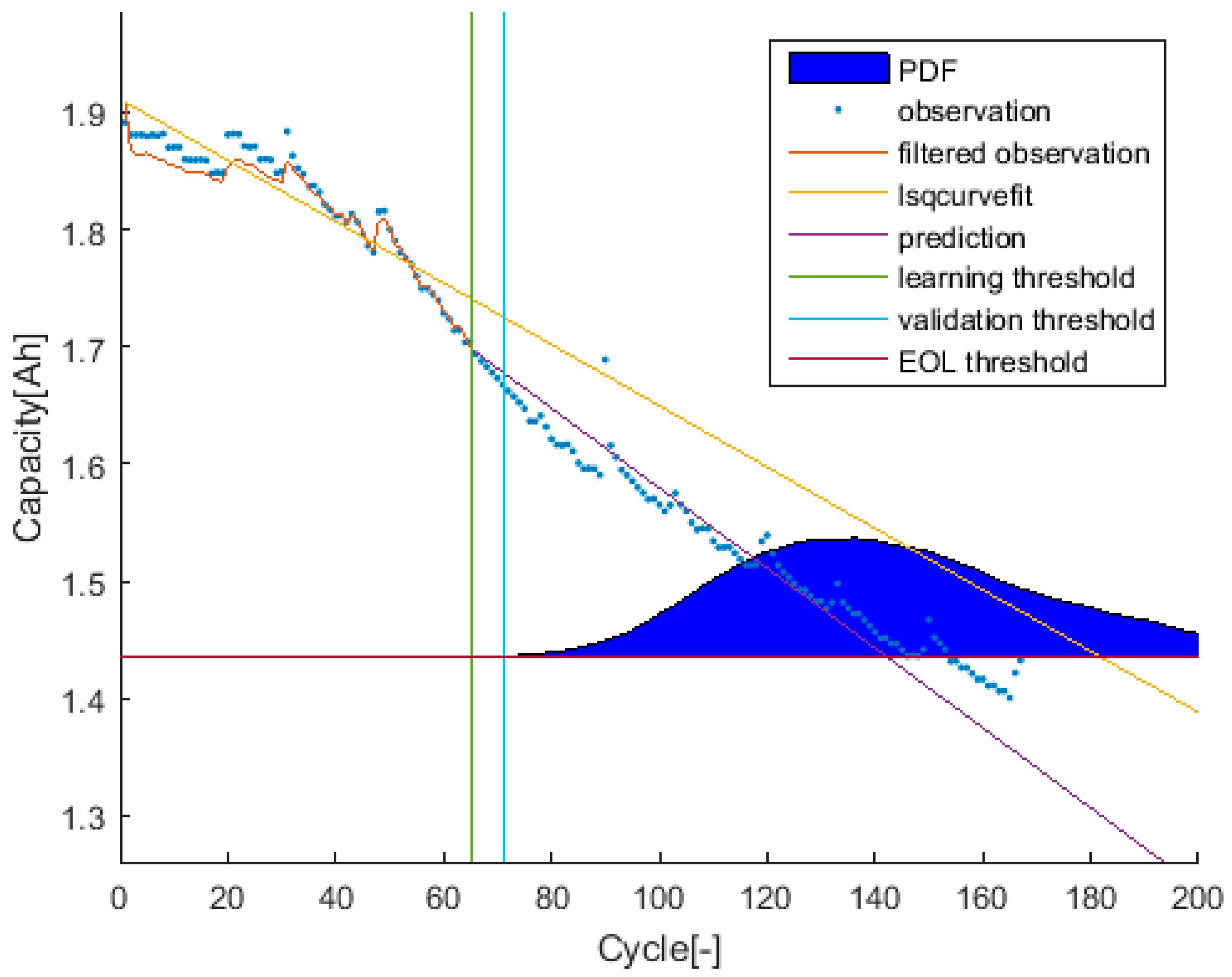
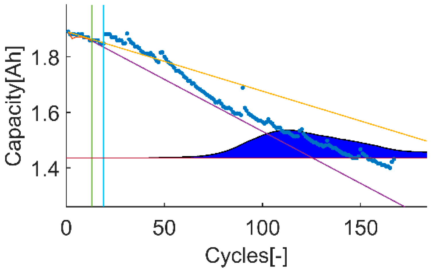
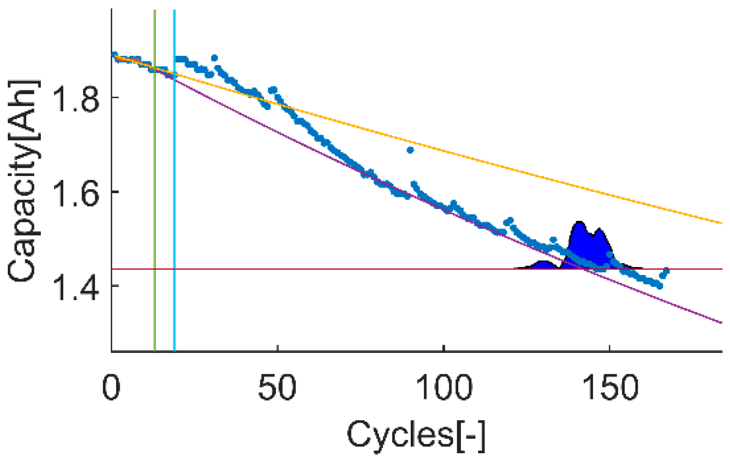
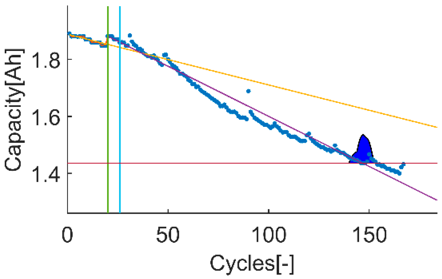
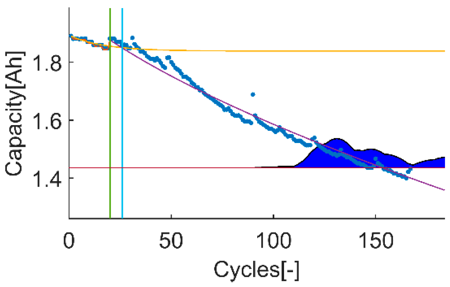
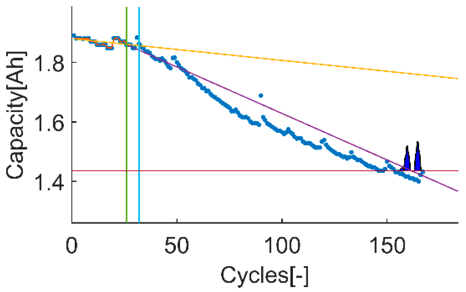
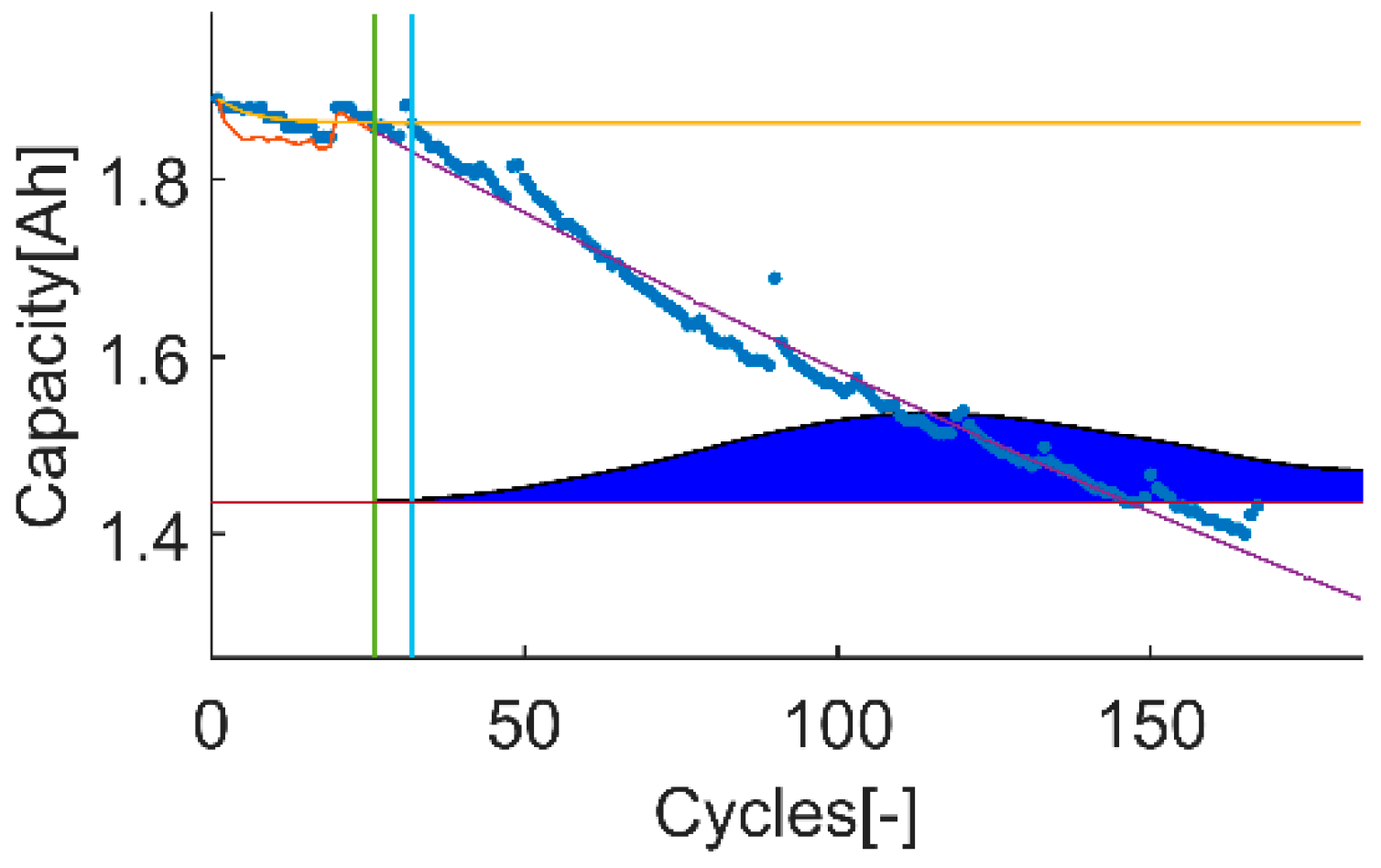
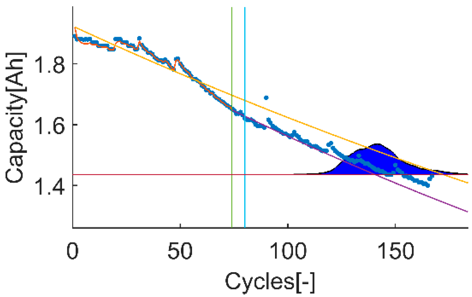
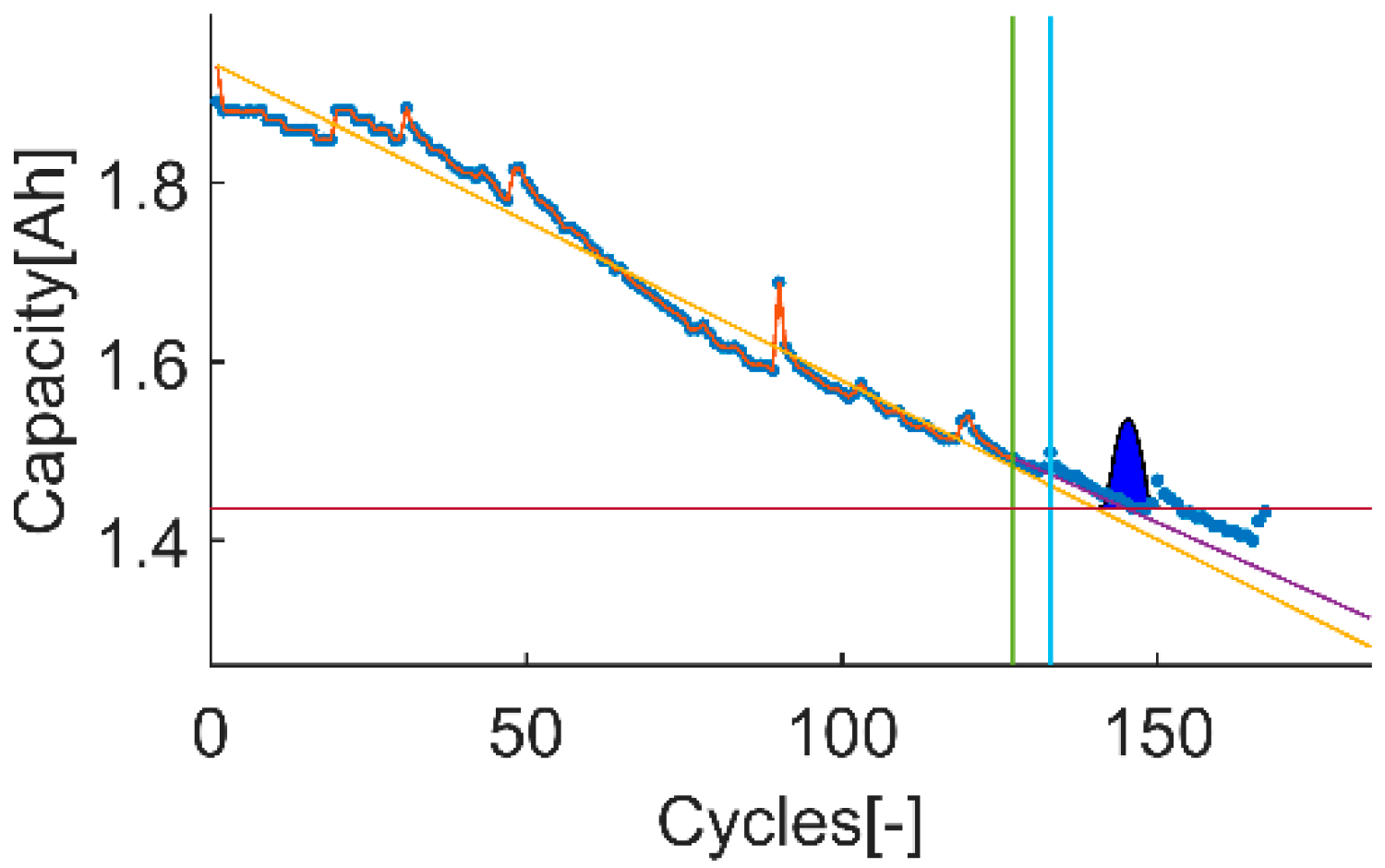
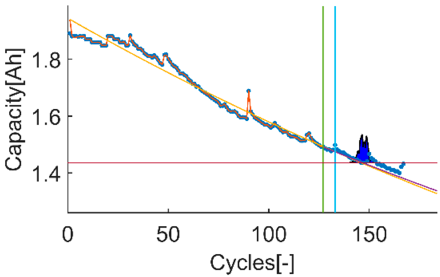
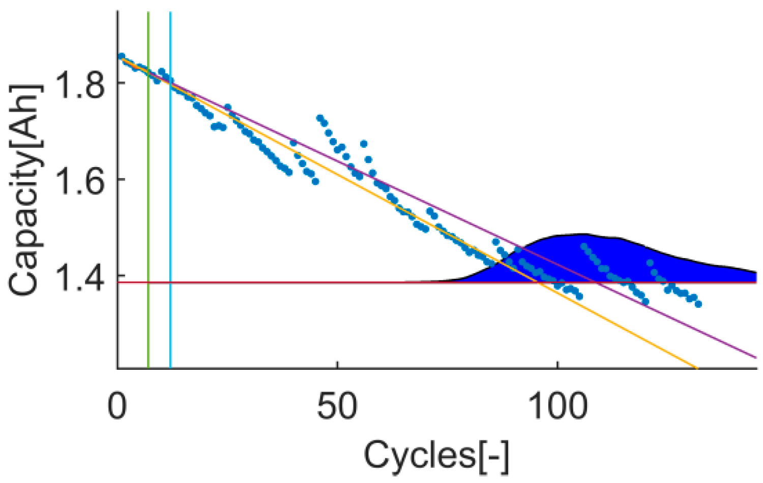
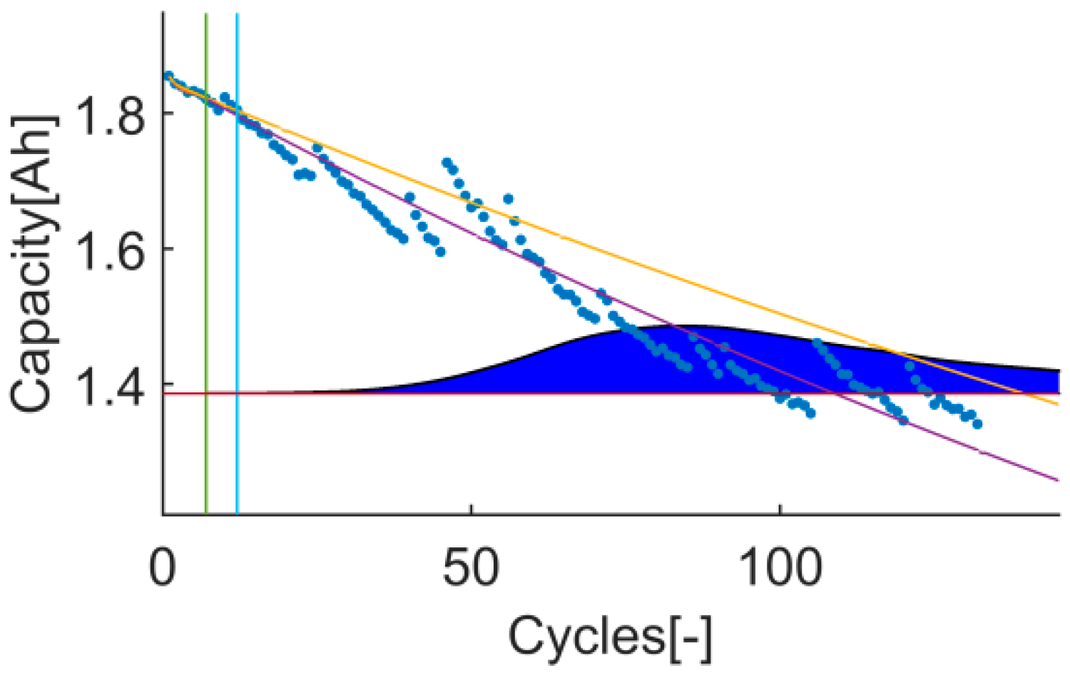
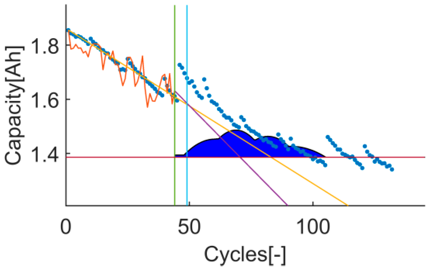
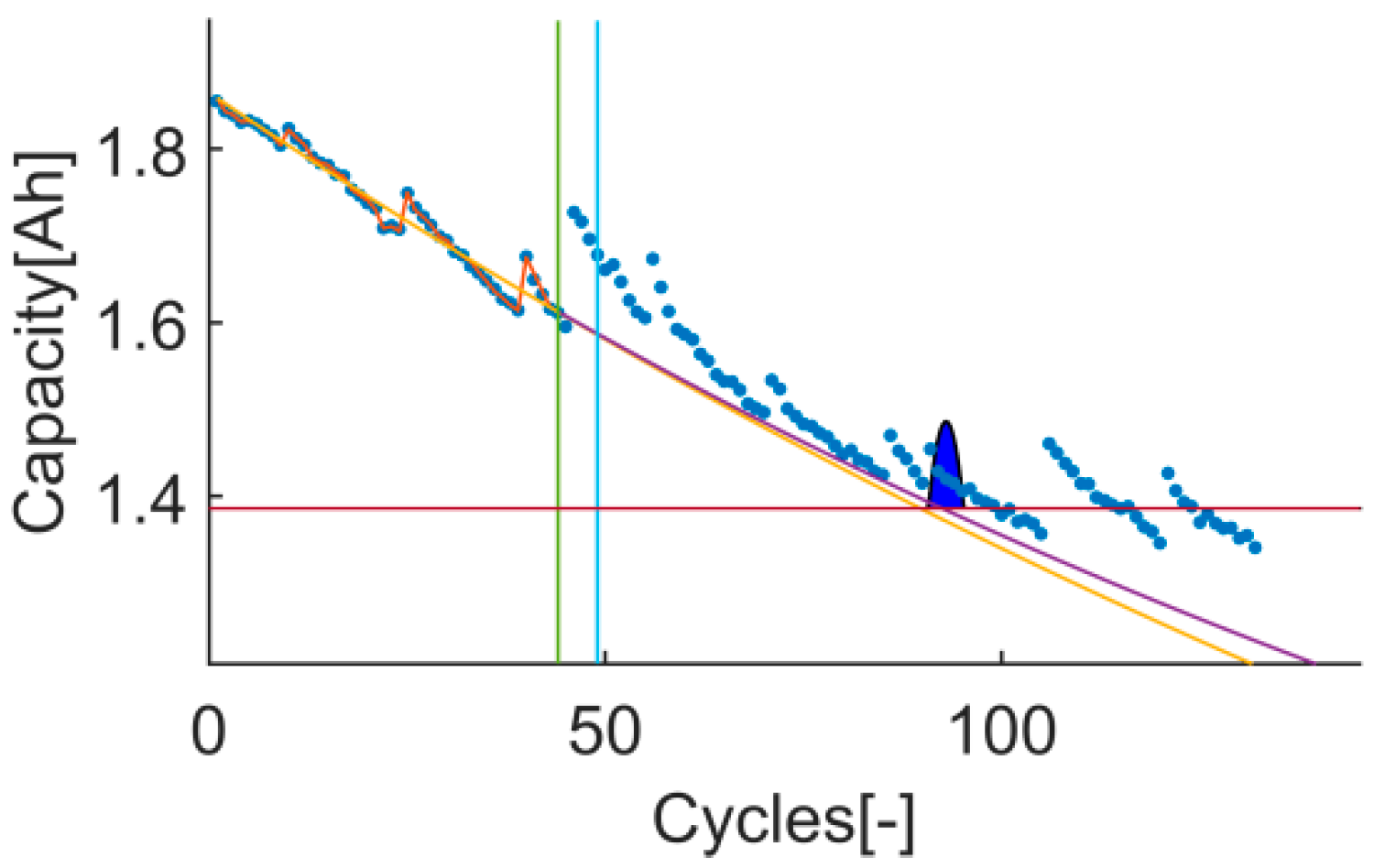
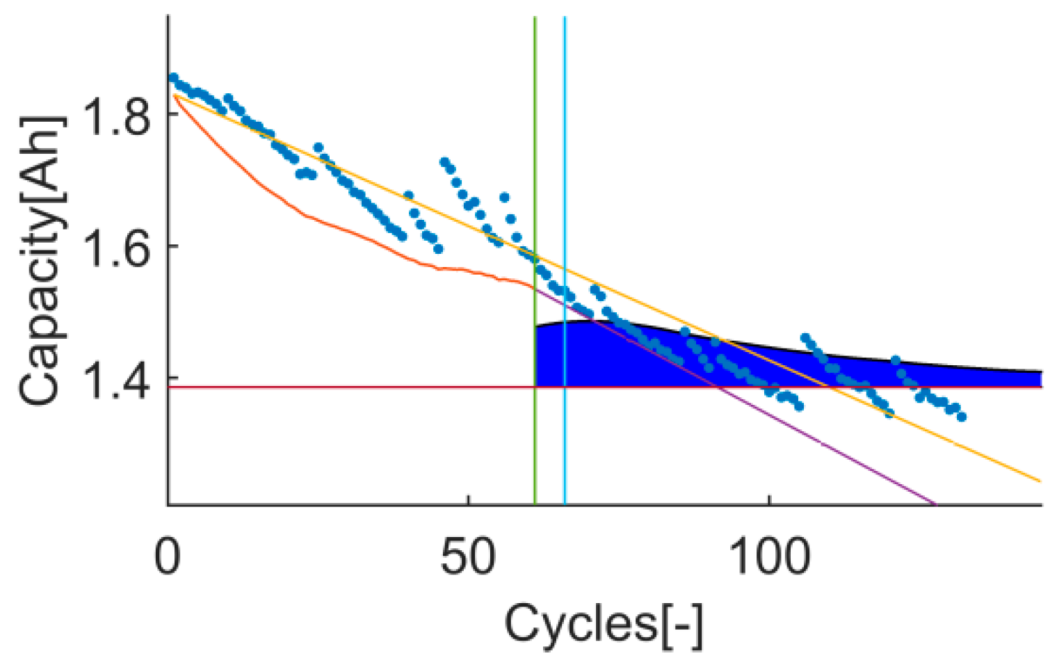
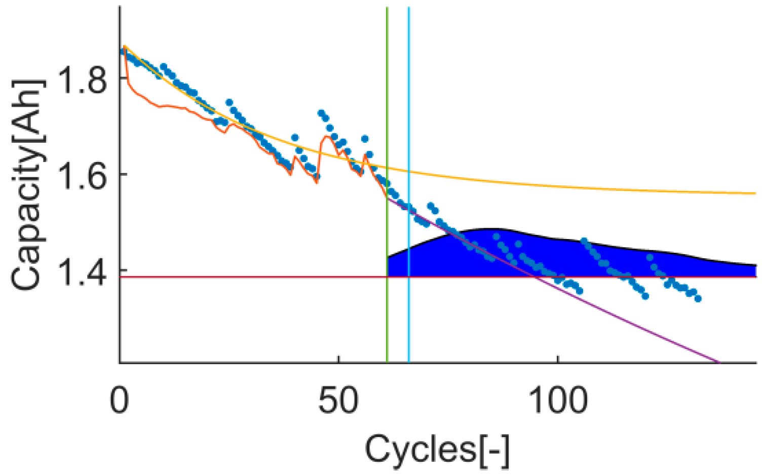
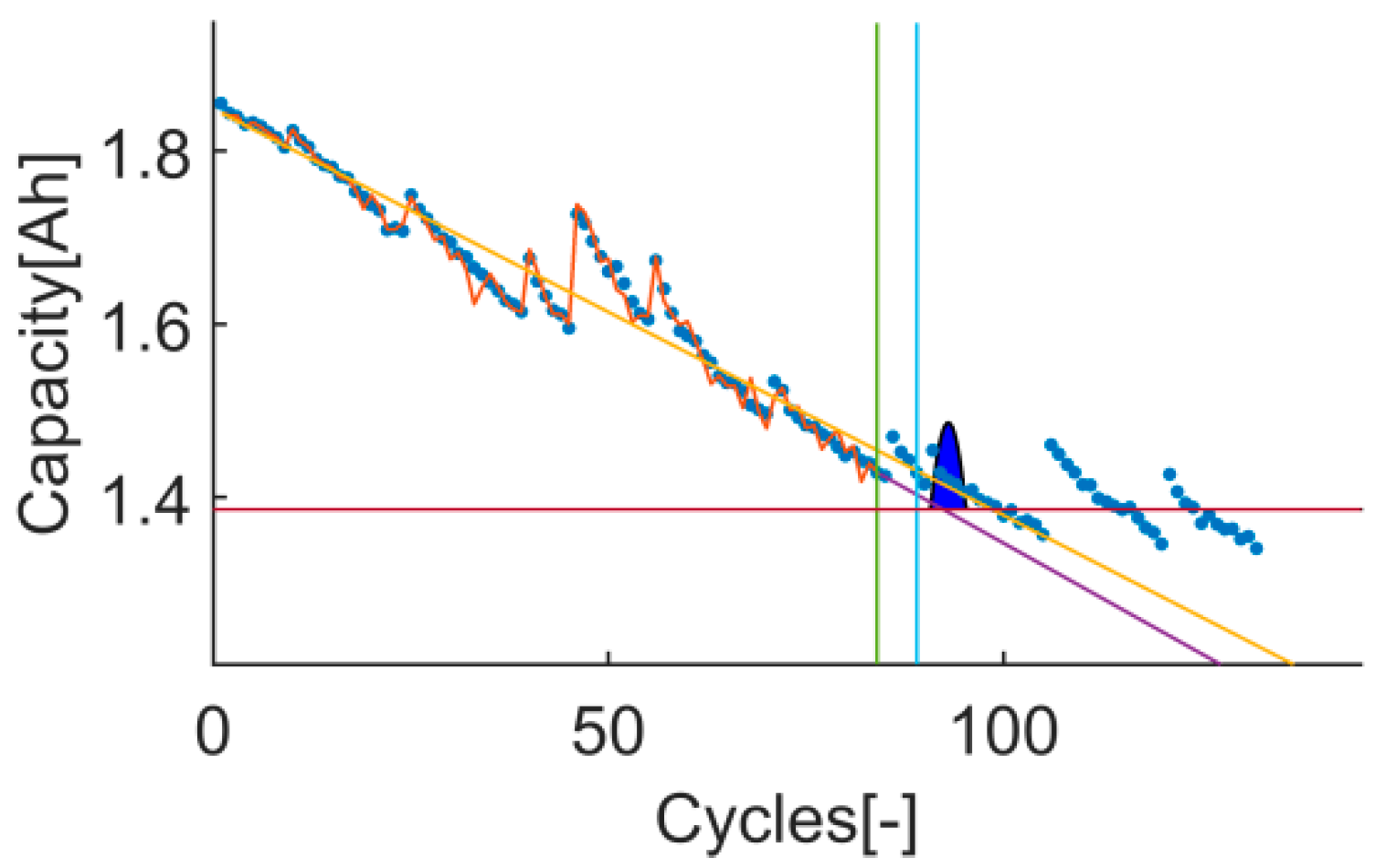
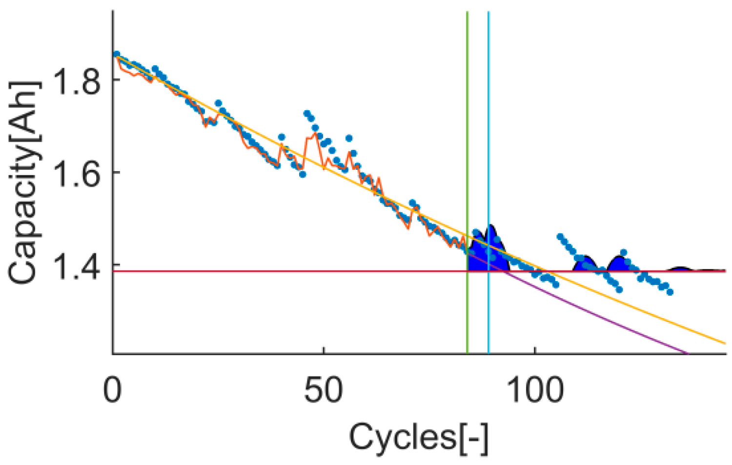
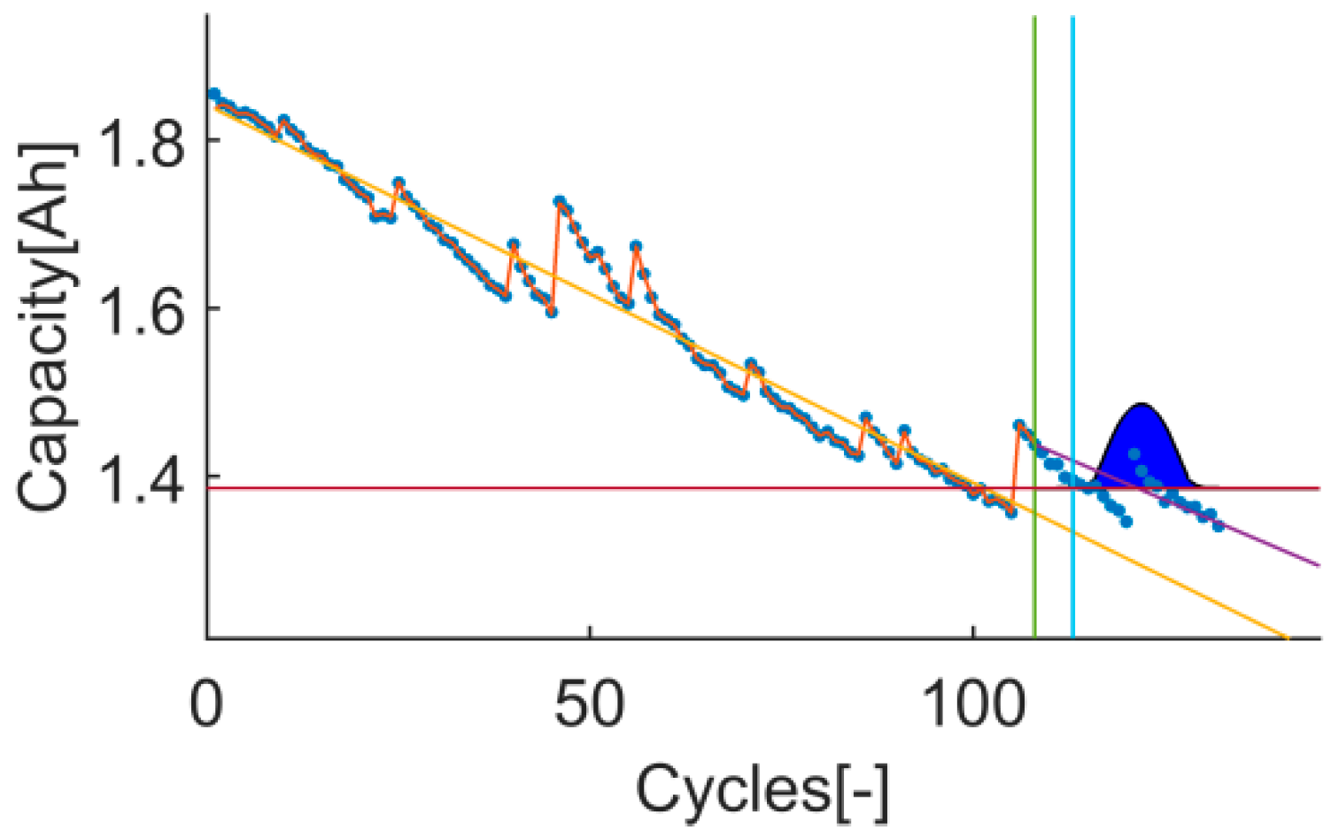
The trial-instant figure shows the response of the algorithm on the whole test data set (training and prediction). This figure displays the training, prediction and EOL thresholds, the inputs (data and prior knowledge) and the output (the response of the algorithm on the whole data set and the RUL distribution). Thanks to this, cases where metrics have estranged values can be further evaluated. This will certainly enrich the discussion, see Figure 2.
2.2.3. Reference Features
This paper develops a standardized language using a unified set of metrics that describe the key attributes of the algorithm, but in order to find the optimal, the attributes of study need to be ranked. For this, some reference values for the proposed metrics are gathered in Table 4.
3. Trial Matrix Design Methodology
The design of the trials is a key aspect when evaluating the features of a stochastic algorithm. It is important to keep in mind that many of the sources of uncertainty on the RUL estimation are “inputs” to the prognostic algorithm [36]. This uncertainty given in form of input may penalize the algorithm in case this input is not correct; it would not be correct to penalize or accept an algorithm according to how well it fits the prediction respect to the ground truth data when the algorithm did not have access to accurate prior knowledge and/or an accurate statement of future conditions. These are the reasons why it is mandatory to develop a rigorous evaluation approach that separates the evaluation of correctness of these “inputs” and the evaluation of the prognostic algorithm itself.
The objective of the proposal is to manage the uncertainty of the “inputs” (data and prior knowledge) with the design of the trials. This will allow evaluating the prognosis algorithm itself. The idea is to apply cases with different level of uncertainty, leading to the illusive “control” of this uncertainty. Firstly, the trial matrix considers data of at least two systems that have different level of noise contribution; and secondly, the trial matrix considers two prior models describing the behavior of the system with different level of accuracy. In this fashion, the correctness of the “inputs” for each algorithm can be discriminated in a certain degree and the evaluation of the prognostic algorithms themselves is improved.
This paper proposes a minimum of a 4 cases trial matrix, shown in Table 5.
4. Universal Parametrization Criteria
The performance level of an algorithm is determined by many factors such as the parameterization. The chosen parameters will define the algorithm’s performance level on a concrete context and goal. However, each algorithm usually has integrated on it its own parametrization method, which does not take into account the context and the goal with which the algorithm needs to work. This leads to evaluate algorithms that are optimized to work on a context different to the interesting one. This paper proposes a universal (applicable to any algorithm) parameterization criterion that corresponds to the context and goals of interest: a RUL prognostic problem context within user specifications with the goal of developing and implementing robust performance assessment algorithms with desired performance levels.
Firstly, the key aspect of the context of interest needs to be defined, which would be “predict a future unknown event”. Next, the parameterization criterion that shares the same key aspect needs to be set. In case of doing a literal interpretation of the key aspect, the parameterization must focus on the future event, but this would go against the purpose of the algorithm since that future event needs to be predicted (needs to be unknown).
In this scenario, some assumptions need to be done. It is assumed that accurate predictions come when the algorithm tracks accurately the future behavior of the system. The key aspect of the context of interest is reformulated as “the tracking of the future behavior of the system”. Thanks to this, the focus of the key aspect that needs to fulfil the algorithm changes from a concrete future event data point to future data in general.
This paper proposes a parametrization criterion based on quantifying the accuracy of the future behavior of the system by a cross validation of a part of the training data set. Since a cross validation is implemented, the part designed for cross validation needs to be removed from the training data set, reducing the amount of data available for training the algorithm. However, thanks to this criterion, a universal parameterization related with its context is achieved.
The validity of the proposed universal parametrization criterion is supported by the states that the parameterization depends on the performance of the algorithm doing predictions (the key aspect of the context is prediction) and by the state that this criterion can be applied to every algorithm designed for RUL prediction.
5. Uncertainty Propagation Method
The uncertainty management is embedded on the stochastic algorithms, which means that each stochastic algorithm has its own way of taking into account the uncertainty [40]. This intrinsic part of the algorithm will impact the precision level that the algorithm achieves.
The proposed evaluation framework has been built on the context of predicting the RUL of the system. This means that the precision evaluation described on Section 2 is quantified from the precision on predicting the RUL. Consequently, the managed uncertainty on the training section needs to be propagated to unknown estimations (to the RUL prediction). However, there are stochastic algorithms that do not have, as an intrinsic characteristic, a way of quantifying the uncertainty on unknown estimations (interpolation or extrapolation), even though being stochastic algorithms (such as the Kalman family stochastic filters). In this scenario, an uncertainty propagation method is proposed in order to cover this deficiency and in order to standardize the uncertainty propagation method under the proposed evaluation framework.
Among the huge variety of uncertainty propagation methods available in the literature [17,21,33], the proposed one is a sampling based method called Monte Carlo prediction [33]. In Monte Carlo prediction, samples from the input distributions are drawn randomly and simulated until the desired event is reached (EOL event), predicting like this the RUL of each sample. The resultant predicted RUL values are weighted depending on the prior probability that each sample had on the input distribution, generating like this a statistic distribution of the predicted RUL. The pseudo-code is available in Algorithm 1.
| Algorithm 1: Monte Carlo Prediction [33]. |
1: for to do 2: 3: 4: 5: 6: 7: end for |
| Where = The event time-instant of th sample. = Number of samples. = The state at th prediction-time-instant (). = The parameter at prediction time knowing the system outputs () at . = Parameter trajectory. = Input trajectory. = Process noise trajectory. = the function to compute . |
Monte Carlo predictions get exact approaches when the number of samples is infinite. This suggests that the higher the number of samples is, the better the approximation will be but the higher the computational burden will be [33]. Therefore, a trade-off between accuracy and computational burden needs to be considered when selecting the number of samples.
6. Example of Use: Definition
The proposed evaluation framework is tested with a stochastic algorithm typically applied on Lithium ion battery RUL prediction problems: the Particle Filter (PF) [4,8,17,24,41]. For that, commonly used inputs are gathered on this example of use. On one hand, the input data is taken from NASA’s data repository [42] and on the other hand, the prior knowledge is obtained from previous studies [4,8,43].
6.1. Stochastic Algorithm
The chosen stochastic algorithm on this example is the Particle Filter (PF). Particle Filter (PF) is a sequential Monte Carlo method. The state Probability Density Function (PDF) is estimated from a set of particles and their associated weights [44]. PF solves the integral operation in the Bayes estimators based on the idea of Monte Carlo method. It estimates the state PDF from a set of particles and their associated weights [5]. The state PDF to its most likely form is adjusted by those weights. As result, an appropriate management of inherent estimation uncertainty is performed [44]. This provides non-linear projection in forecasting [45].
The particles are inferred recursively by two alternate phases. The first phase is the prediction. In the prediction, the values of the particles at the next step are estimated using the values of the particles at the previous step. There is not any involvement of neither measurement nor observation in this step. The second phase is the update. In the update, the value of each particle estimated in the prediction phase is compared with the measurements. Afterwards, the value of the particles is updated accordingly [44]. As an initialization step (), the proposed PF draws the particles from a Gaussian distribution () and calculates the weights from a uniform distribution ().
However, PF has two main problems: Particle degradation and sample impoverishment. To lessen the impact of particle degradation, a system importance resampling of the particles is carried out on the iterations that do not reach the pre-set resampling threshold. This helps in maintaining the track of the state vector even when disruptive effects like un-modelled operational conditions appear [39]. The pseudo-code of the PF is shown in Algorithm 2.
| Algorithm 2: Sample Importance Resampling Particle Filter [46]. |
1: for to do 2: 3: 4: end for 5: 6: for to do 7: 8: end for 9: 10: If then 11: 12: end if |
| Where = The state of the th particle at time-instant. = The weight of th particle at time-instant. = Number of particles. = The input at time-instant. = The output at time-instant. = Cumulative weight. = Effective number of particles. = User defined threshold of effective number of particles. |
Among the possibilities on system importance resampling methods, the “systematic resampling method”, the “stratified resampling method” and the “multinomial resampling method” are the most typical methods [47]. Among them, the chosen algorithm has been the “systematic resampling method” because it is the most common one [46] and because there is no big difference on the obtained results with any of these typical methods on the proposed evaluation framework [25]. The pseudo-code of the “systematic resampling method” is shown in Algorithm 3.
| Algorithm 3: Systematic Resampling [48]. |
1: 2: for to do 3: 4: end for 5: 6: 7: for to do 8: 9: while do 10: 11: end while 12: 13: 14: end if |
| Where = The state of the th particle at time-instant. = The weight of th particle at time-instant. = Number of particles. = The cumulative sum of the weight of the particles until th particle at time-instant. = Step reference for searching the particles that will be used before the resampling. |
6.2. Input
In this proposal, the input of the algorithm refers to the information of the system that is under evaluation: the information about the lithium-ion battery that is introduced into the stochastic algorithm to predict the event of interest. In this case, the event of interest is the EOL. The EOL is commonly defined as a specific dischargeable capacity value, whose behavior is commonly described by an aging model. Consequently, the dischargeable capacity data as well as the aging model that describes the evolution observed on that data are the input of the algorithm.
6.2.1. Data
The dischargeable capacity values are taken from NASA’s data repository [42], a repetitively used public data source on evaluating Lithium-ion battery RUL prognosis algorithms. The selected NASA’s data sets consist of rechargeable 18650 Gen 2 Li-ion cells with a rated capacity of 2 Ah. The experiment description is taken literally from [49] as follows: “It was conducted through three different operational profiles (charge, discharge and impedance) at room temperature. Charging was performed in a constant current at 1.5 A until the battery voltage reached 4.2 V and continued in constant voltage mode until the charge current dropped to 20 mA. The discharge runs were stopped at 2.7 V. The experiments were conducted until the capacity decreased to the specified EOL criteria of 1.4 Ah”.
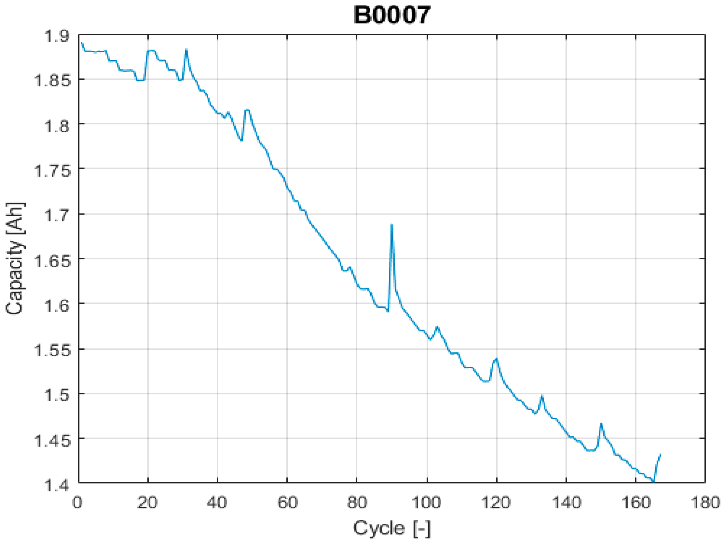
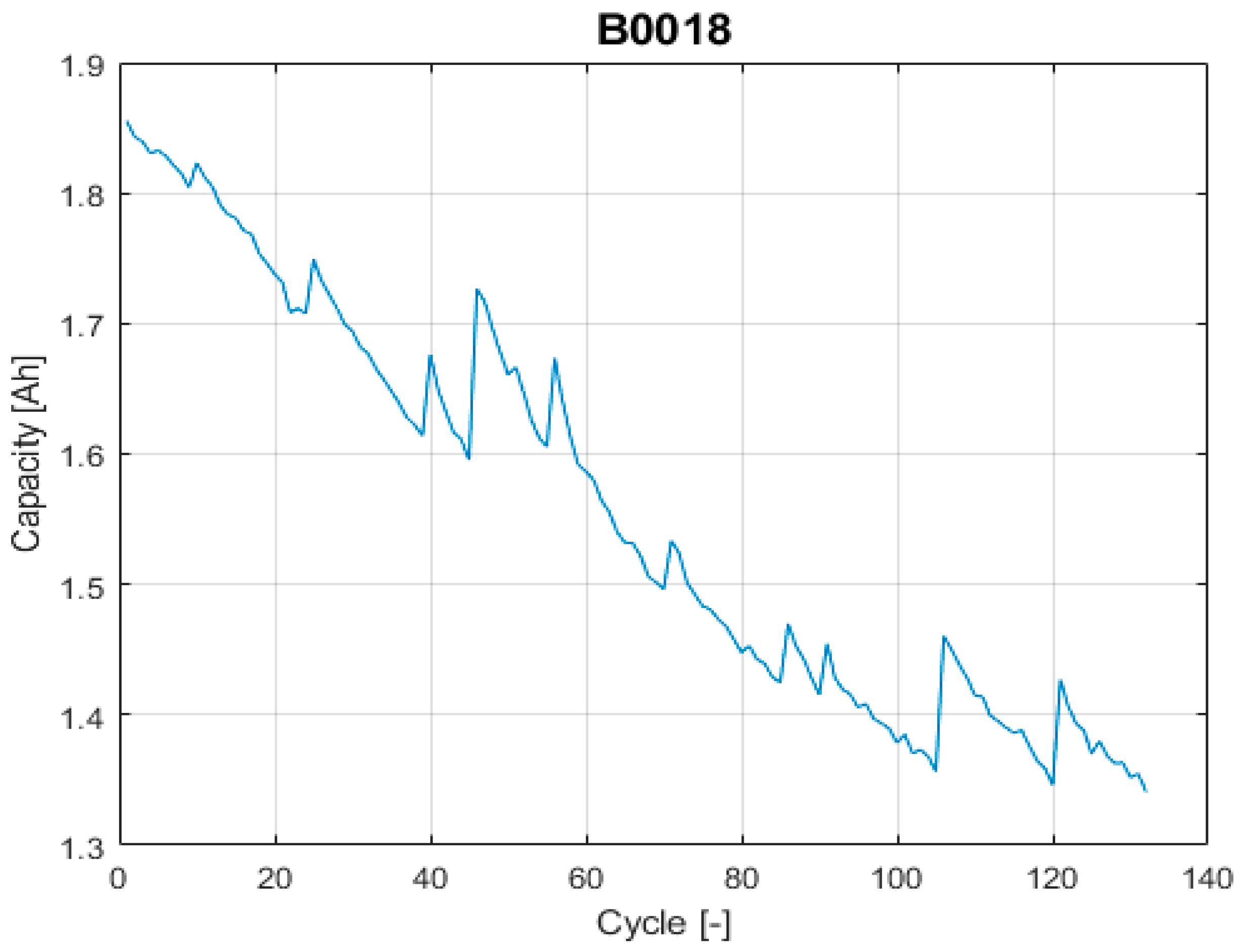
Among the different data sets available on the selected NASA’s data repository, the proposed evaluation framework requires using two data sets with different uncertainty levels on the data itself. To do end, it is considered that the uncertainty on the input data comes from the effects that the proposed models on the prior knowledge section (next section) cannot completely describe, such as the capacity recovery events. Based on this, the selected data set with high uncertainty is “B0018” and the selected data set with low uncertainty is “B0007”, see Figure 3 and Figure 4.
6.2.2. Prior Knowledge
The behavioral aspect that needs to be modelled by the prior knowledge would be the dischargeable capacity evolution of the battery until, at least, the EOL event. In lithium-ion battery, the dischargeable capacity suffers a decreasing evolution or a decay. For that, the selected prior knowledge describes two aspects of the behavior of the selected lithium-ion battery: the capacity decay (also referred as the aging model) and the state transition model on that capacity decay.
For the capacity decay, this paper proposes to use two semi-empirical capacity decrease models that have different uncertainty levels on describing the system’s behavior. In the literature, it has been proved that the capacity decay is non-linear [43] and that a double exponential expression is able to describe the capacity decay behavior with a high level of confidence [4,8]. Therefore, a double exponential model is taken as the prior knowledge with low uncertainty (Equation (11)), and a linear model is taken as the prior knowledge with high uncertainty (Equation (12)).
For the state transition model, a linear stochastic process is proposed as the state transition model of the parameters for both capacity decrease models (Equation (13)). In this case, the uncertainty of this part of the prior knowledge is quantified by the parametrization algorithm; therefore, uncertainty evaluation of this part of the input is not required and thus, a second model is not used.
6.3. Trial Matrix
The whole trial matrix that follows the proposed cases is shown in Table 6.
6.4. Parametrization
Firstly, a parameter definition step has been done based on experience and on the literature [23,26,50]. The defined parameters are resumed in Table 7.
Then, the parameterization of the hyper-parameters of the algorithm is performed (Algorithm 4). It starts initializing the inner states at each time-instant. For that, a “least squares optimization” of the training data and the capacity decay model is conducted using MATLAB’s “lsqcurvefit” function. Once done this, the algorithm’s hyper-parameters at each time step (Table 8) are achieved by grid search optimization.
The grid for each hyper-parameter is designed based on the rule of delimiting as much as possible the tested values without losing interesting options. For that, a sensibility analysis would be required, but in this case, the design of the grid is based on previous engineering experience. The obtained results have led to define the limits of the grids as well as defining the grid delta values. The created grids are shown in Table 9.
The results obtained with every configuration on the grid are evaluated to find the optimal hyper-parameters. This is done running Cv times each grid configuration and finding the case with the lowest variation among the run cases with the lowest RMSE values on the cross-validation data set.
| Algorithm 4: Parameterization. |
1: for to 2: for to do 3: for to do 4: for to do 5: for to do 6: 7: 8: 9: for to do 10: 11: end for 12: 13: end for 14: end for 15: end for 16: end for 17: 18: 19: end for |
| Where = The optimum hyper-parameters in prediction-time-instant. = The time-instants from initial time to prediction time . = Amount of prediction-time-instants under evaluation. = Amount of repetitions of each configuration on the grid. = Amount of learning points in th prediction-time-instant. = Root Mean Square Error in each iteration of the grid search optimization. = The state of the th particle at time-instant. = The weight of th particle at time-instant. = Number of particles. = The input at time-instant. = The output at time-instant. = The output in prediction-time-instant. = Prediction of the output in prediction-time-instant on the validation data set. = The grid of the hyper-parameter . = The top ten hyper-parameters in prediction-time-instant in each repetition . |
7. Example of Use: Results and Discussion
The selected stochastic algorithm (Algorithm 2) along with the proposed uncertainty propagation method (Algorithm 1) is applied on all the described trials (Table 6). The achieved values of the quantitative metrics described in Table 2 and Table 3 are shown in Table 10. In addition, the achieved qualitative prognosis results are shown on four figures that display the PH and α-λ accuracy (Figure 5, Figure 6, Figure 7 and Figure 8). These results allow the overall evaluation of the algorithm.
The highest PH values are calculated on the tests 2 and 4 with a “perfect” one. This means that the tracking of the correct aging trend underneath of the data set B0018 can be done in the earliest selected prediction-time-instant. The test 1 and 3 shows lower PH values than the obtained in the tests 2 and 4. However, the obtained scores are above 0.8, which are high values by themselves. In this case, the test 3 shows a higher value than the test 4. This means that the algorithm with the exponential model fits better the model response on early states.
The CRA values are much higher on the tests 1 and 3 compared with the CRA values obtained on tests 2 and 4. This means that the achievable RA improves in a much higher rate on the data set B0007 than B0018 (as expected, since the data set B0018 has higher uncertainty than the data set B0007). The highest CRA value is achieved on the test 3, which means that the algorithm works better on the data set B0007 with the exponential model. In contrast, the lowest CRA value is achieved on the test 4, which means that the prediction algorithm works worst on the data set B0018 with the exponential model. This means that the exponential fits better the data set B0007 than the linear model but that for the data set B0018, the model that fits better the data set is the linear model.
In terms of computational burden, the tests 3 and 4 have higher number of FLOPs than 1 and 2, which means that the exponential model needs more computational resources than the linear model. In the same way, the length of the data sets also influences, being the one with more data points the ones with more FLOPs.
Once the overall evaluation of the algorithm has been done, some prediction-time-instants () of high interest have been analysed in more detail; specially, the tests run on the data set B0007 at 4, 11, 17, 65 and 118 prediction-time-instants. For that, the quantitative metrics described in Table 1 are used. The results of those prediction-time-instants are shown in Table 11, Table 12, Table 13 and Table 14. Furthermore, some of the trial-instant figures have been displayed for further interpretation of the obtained results.
- t11: The prediction RMSE, the RA, the Pvalue and the Pwidth are better in test 1. In this case, the values of this 4 metrics on t11 are against the obtained results from the PH evaluation. The training data set is still small and there is an event that the model is not able to describe (a capacity recovery event). The data set under evaluation here could be labelled as a data set with high uncertainty since the chosen models are not able to describe the behavior on the validation data set using the tracked behavior on the training data set. As a result, the simplest model (the linear model) works better than the exponential one, see Figure 11 and Figure 12.
- t17: The prediction RMSE and the RA of the test 3 are better than the ones of the test 1. However, the Pwidth in test 3 is 1.78, which exceeds the upper limit of ideal range by 78%. A Pwidth higher than 1 means that the uncertainty is higher than the real RUL on that t2, which is a sign of overestimating the uncertainty and therefore, the prediction is not precise. On the other hand, test 1’s Pvalue is 0 (even though the Pwidth is in between the ideal range), which means that, in this case, the uncertainty has been underestimated. In both cases the prediction is not precise; see Figure 13 and Figure 14.
- t65: The prediction RMSE, the RA, the Pvalue and the Pwidth are better in test 3. The results are in line with the conclusions drawn from the CRA evaluation; there is a greater improve on the results related with the accuracy on test 3. Besides, the Pvalue of test 1 is 0.06, which means that the uncertainty is underestimated and therefore, the prediction is not precise, see Figure 15 and Figure 16.
- t118: The RA and the Pwidth are the same on both cases but the prediction RMSE and the Pvalue are worse in test 1. This means that the test 3 has a higher probability of predicting the real RUL and that tracks better the nearest trend. The exponential model describes better the trend underneath the data, see Figure 17 and Figure 18.
The chosen cases on the tests run on the data set B0018 are the results obtained at 1, 38, 55, 78 and 102 prediction-time-instants:
- t1: The prediction RMSE, the RA, the Pvalue and the Pwidth are close to the idle cases defined on Table 4. Thanks to these high rates, the prediction has fulfilled the α-bound requirement of the PH, leading to have perfect PH values of 1. The values of this 4 metrics on t1 are in line with the conclusions drawn from the PH evaluation, see Figure 19 and Figure 20.
- t38: The prediction RMSE and the RA are better in test 4 but the in both tests are equal to 0. The RA values in both cases are too low, which leads to have low probabilities on predicting the RUL. There is a huge capacity recovery event on the validation data set used on the parametrization, which cannot be described by the selected models (the behavior on the validation data set cannot be described by using the tracked behavior on the training data set). As a result, we were expecting to have better response with the simplest model as in prediction-time-instant of tests 1 and 3 (Figure 11 and Figure 12). However, in this case we have seen that the incapability of describing the underneath trend of the validation data set by using the tracked underneath trend of the training data set has led to an instable response of the algorithm due to a wrong parametrization, see Figure 21 and Figure 22.
- t55: The prediction RMSE, the RA, the Pvalue and the Pwidth are better in test 4. In both cases the RA and the Pvalue are far from the perfect score. This means that both models do not track properly the trend underneath the data. This is most likely due to the high uncertainty level on the data set seen by the algorithm (training data set), see Figure 23 and Figure 24.
- t78: In both tests, the prediction RMSE and the RA are far away from the optimal values described in Table 4. The training data set in t78 is composed by more than half of the data set, but instead of getting better results, the results are worse. The results are in line with the conclusions drawn from the CRA evaluation; the prediction does not increase even though increasing the training data set as well as in tests 1 and 3, see Figure 25 and Figure 26.
- t102: In both tests, the prediction RMSE is close to the “best” cases defined on Table 4, but the other three metrics are way too far away from the optimal values even though being close to the event-time-instant of interest. This supports the fact of having such differences between the CRA values of test 1–3 and 2–4. As well, it supports the first assumption of defining the data set B0018 as highly uncertain and B0007 lowly uncertain. See Figure 27 and Figure 28.
Evaluating the qualitative graphs, we can draw qualitatively the conclusions done on the qualitative evaluation and confirm them in a friendlier way.
It can be seen how the tests 2 and 4 have on the first time-instant a RUL prediction inside the α-bounds, generating a high PH value even though having most of the rest of the RUL prediction out of the α-boundaries. There are much more cases that fulfils the α-boundaries of the PH and α-λ accuracy on the tests 1 and 3 and that the response on these two tests is improved when increasing the training data points. In contrast, the results on the tests 2 and 4 show kind of an offset on the obtained accuracy, which do not seem to improve even though increasing the training data set.
Checking on the same data set, it looks like the results on the test 3 are better than the results on the test 1 and that the results on the test 2 are better than the results on the test 4. This can be interpreted as being the linear model a better prior knowledge for highly uncertain data sets, even though knowing that the behavior of the trend underneath the data is exponential [39,43].
8. Conclusions
This paper presents an algorithm evaluation framework that captures the performance level of any stochastic algorithm. It combines existing seven quantitative metrics and two qualitative diagrams. The evaluation framework is contextualized in a concrete application environment: a prognosis problem of a lithium-ion battery. The approach is characterized in detail, where the effect of usually forgotten variables are analyzed and dealt with the uncertainty contribution of the inputs on the estimations, the used parametrization method, and the uncertainty propagation method. The analysis of these three variables composes the main innovative contribution of this paper. Finally, the framework has been tested on a Particle Filter (PF) applied in a lithium-ion battery prognosis problem.
The proposed evaluation method has shown that both, the correctness and timeliness need to be analyzed in order to capture completely the prognosis algorithms performance level. The evaluation of the PF has shown that the correctness results on a specific prediction-time-instant do not correctly represent the obtainable correctness on some other prediction-time-instant. Therefore, the timeliness analysis is necessary. However, the timeliness cannot describe the algorithms performance level by itself. The results have shown that the PH or the CRA are not able to determine the accuracy or precision with which the algorithm can predict. Therefore, the evaluation of the correctness and timeliness of the algorithm is required.
Additionally, we have seen that the proposed qualitative graphs help considerably the interpretation of the obtained results. The use of these graphs is not necessary since the quantitative metrics alone are able to capture and quantify the performance level of the algorithm. Nonetheless, the use of these graphical aids is highly recommendable.
The acquired results from the evaluation of the PF have shown that the data set influences greatly the response of the selected algorithm (in average, the results on the ‘B0018′ data set are way worse than the results on the ‘B0007′ data set). The characteristics of the data set have a relevant effect on the obtainable results of that prognosis algorithm. Therefore, the use of data sets with different level of uncertainty is essential when evaluating the performance level of a prognosis algorithm.
The adopted parametrization criterion allows us to determine the hyper-parameters of any prognosis algorithm on every prediction-time-instant. Nonetheless, it shows that depending on the characteristics of the data set on the different evaluated prediction-time-instants, the hyper-parameters cannot be obtained. This can be used to reduce the evaluated prediction-time-instants. Thanks to this, completely random or inaccurate predictions due to the intrinsic characteristics of the training data set will be avoided. Furthermore, we are able to identify the time-instants with accurate predictions, which is really interesting for on-board applications.
The proposed uncertainty propagation method based on Monte-Carlo simulations generates the probability distributions based on random RUL estimations. This method allows us to use the same approach to propagate the uncertainty on any prognosis algorithm, standardizing like this the uncertainty propagation method. Besides, it provides an uncertainty propagation method to those stochastic algorithms that do not have a proper uncertainty propagation method, such as the Kalman family stochastic filters.
Author Contributions
Conceptualization, M.A., M.O. and E.M.; methodology, M.A.; software, M.A.; writing—original draft preparation, M.A.; writing—review and editing, M.A., M.O., E.M. and H.M.; supervision, M.O. and E.M. All authors have read and agreed to the published version of the manuscript.
Funding
This research received no external funding.
Institutional Review Board Statement
Not applicable.
Informed Consent Statement
Not applicable.
Data Availability Statement
Not applicable.
Conflicts of Interest
The authors declare no conflict of interest. The funders had no role in the design of the study; in the collection, analyses, or interpretation of data; in the writing of the manuscript, or in the decision to publish the results.
References
- Rezvanizaniani, S.M.; Liu, Z.; Chen, Y.; Lee, J. Review and recent advances in battery health monitoring and prognostics technologies for electric vehicle (EV) safety and mobility. J. Power Sources 2014, 256, 110–124. [Google Scholar] [CrossRef]
- Widodo, A.; Shim, M.-C.; Caesarendra, W.; Yang, B.-S. Intelligent prognostics for battery health monitoring based on sample entropy. Expert Syst. Appl. 2011, 38, 11763–11769. [Google Scholar] [CrossRef]
- Li, S.; Pischinger, S.; He, C.; Liang, L.; Stapelbroek, M. A comparative study of model-based capacity estimation algorithms in dual estimation frameworks for lithium-ion batteries under an accelerated aging test. Appl. Energy 2018, 212, 1522–1536. [Google Scholar] [CrossRef]
- Zhang, H.; Miao, Q.; Zhang, X.; Liu, Z. An improved unscented particle filter approach for lithium-ion battery remaining useful life prediction. Microelectron. Reliab. 2018, 81, 288–298. [Google Scholar] [CrossRef]
- Zhang, X.; Miao, Q.; Liu, Z. Remaining useful life prediction of lithium-ion battery using an improved UPF method based on MCMC. Microelectron. Reliab. 2017, 75, 288–295. [Google Scholar] [CrossRef]
- Liu, D.; Zhou, J.; Liao, H.; Peng, Y.; Peng, X. A Health Indicator Extraction and Optimization Framework for Lithium-Ion Battery Degradation Modeling and Prognostics. IEEE Trans. Syst. Man Cybern. Syst. 2015, 45, 915–928. [Google Scholar] [CrossRef]
- Wang, D.; Miao, Q.; Pecht, M. Prognostics of lithium-ion batteries based on relevance vectors and a conditional three-parameter capacity degradation model. J. Power Sources 2013, 239, 253–264. [Google Scholar] [CrossRef]
- Duong, P.L.T.; Raghavan, N. Heuristic Kalman optimized particle filter for remaining useful life prediction of lithium-ion battery. Microelectron. Reliab. 2018, 81, 232–243. [Google Scholar] [CrossRef]
- Liu, D.; Luo, Y.; Peng, Y.; Peng, X.; Pecht, M. Lithium-ion Battery Remaining Useful Life Estimation Based on Nonlinear AR Model Combined with Degradation Feature. Annu. Conf. Progn. Health Manag. Soc. 2012, 3, 1803–1836. [Google Scholar]
- Johnen, M.; Pitzen, S.; Kamps, U.; Kateri, M.; Dechent, P.; Sauer, D.U. Modeling long-term capacity degradation of lithium-ion batteries. J. Energy Storage 2021, 34, 102011. [Google Scholar] [CrossRef]
- Jia, J.; Liang, J.; Shi, Y.; Wen, J.; Pang, X.; Zeng, J. SOH and RUL Prediction of Lithium-Ion Batteries Based on Gaussian Process Regression with Indirect Health Indicators. Energies 2020, 13, 375. [Google Scholar] [CrossRef] [Green Version]
- Wang, H.; Song, W.; Zio, E.; Kudreyko, A.; Zhang, Y. Remaining useful life prediction for Lithium-ion batteries using fractional Brownian motion and Fruit-fly Optimization Algorithm. Meas. J. Int. Meas. Confed. 2020, 161, 107904. [Google Scholar] [CrossRef]
- Li, F.; Xu, J. A new prognostics method for state of health estimation of lithium-ion batteries based on a mixture of Gaussian process models and particle filter. Microelectron. Reliab. 2015, 55, 1035–1045. [Google Scholar] [CrossRef]
- He, Y.-J.; Shen, J.-N.; Shen, J.-F.; Ma, Z.-F. State of health estimation of lithium-ion batteries: A multiscale Gaussian process regression modeling approach. AIChE J. 2015, 61, 1589–1600. [Google Scholar] [CrossRef]
- Zhou, D.; Yin, H.; Fu, P.; Song, X.; Lu, W.; Yuan, L.; Fu, Z. Prognostics for State of Health of Lithium-Ion Batteries Based on Gaussian Process Regression. Math. Probl. Eng. 2018, 2018, 1–11. [Google Scholar] [CrossRef] [Green Version]
- Wei, J.; Dong, G.; Chen, Z. Remaining Useful Life Prediction and State of Health Diagnosis for Lithium-Ion Batteries Using Particle Filter and Support Vector Regression. IEEE Trans. Ind. Electron. 2018, 65, 5634–5643. [Google Scholar] [CrossRef]
- Zhang, L.; Mu, Z.; Sun, C. Remaining Useful Life Prediction for Lithium-Ion Batteries Based on Exponential Model and Particle Filter. IEEE Access 2018, 6, 17729–17740. [Google Scholar] [CrossRef]
- Saxena, A.; Celaya, J.; Saha, B.; Saha, S.; Goebel, K. Metrics for Offline Evaluation of Prognostic Performance. Int. J. Progn. Health Manag. 2010, 1, 1–20. [Google Scholar] [CrossRef]
- Saxena, A.; Goebel, K.; Simon, D.; Eklund, N. Damage propagation modeling for aircraft engine run-to-failure simulation. In Proceedings of the 2008 International Conference on Prognostics and Health Management, Denver, CO, USA, 6–9 October 2008. [Google Scholar]
- Tang, L.; Orchard, M.E.; Goebel, K.; Vachtsevanos, G. Novel metrics and methodologies for the verification and validation of prognostic algorithms. In Proceedings of the 2011 Aerospace Conference 2011, Big Sky, MT, USA, 5–12 March 2011; pp. 1–8. [Google Scholar]
- Acuña, D.E.; Orchard, M.E. Prognostic Algorithms Design Based on Predictive Bayesian Cramér-Rao Lower Bounds. IFAC-PapersOnLine 2017, 50, 4719–4726. [Google Scholar] [CrossRef]
- Richardson, R.R.; Osborne, M.; Howey, D.A. Battery health prediction under generalized conditions using a Gaussian process transition model. J. Energy Storage 2019, 23, 320–328. [Google Scholar] [CrossRef]
- Pugalenthi, K.; Raghavan, N. A holistic comparison of the different resampling algorithms for particle filter based prognosis using lithium ion batteries as a case study. Microelectron. Reliab. 2018, 91, 160–169. [Google Scholar] [CrossRef]
- Miao, Q.; Xie, L.; Cui, H.; Liang, W.; Pecht, M. Remaining useful life prediction of lithium-ion battery with unscented particle filter technique. Microelectron. Reliab. 2013, 53, 805–810. [Google Scholar] [CrossRef]
- Arrinda, M.; Oyarbide, M.; Macicior, H.; Muxika, E. Comparison of Stochastic capacity estimation tools applied on remaining useful life prognosis of Lithium ion batteries. PHM Soc. Eur. Conf. 2018, 4. [Google Scholar] [CrossRef]
- Saxena, A.; Celaya, J.R.; Saha, B.; Saha, S.; Goebel, K. On Applying the Prognostic Performance Metrics. Annu. Conf. Progn. Health Manag. Soc. 2009, 9, 1–16. [Google Scholar]
- Rathnapriya, S.; Manikandan, V. Remaining Useful Life Prediction of Analog Circuit Using Improved Unscented Particle Filter. J. Electron. Test. 2020, 36, 169–181. [Google Scholar] [CrossRef]
- Ha, Y.; Zhang, H. Fast multi-output relevance vector regression. Econ. Model. 2019, 81, 217–230. [Google Scholar] [CrossRef] [Green Version]
- Zhao, L.; Li, Q.; Suo, B. Simulator Assessment Theory for Remaining Useful Life Prediction of Lithium-Ion Battery Under Multiple Uncertainties. IEEE Access 2020, 8, 71447–71459. [Google Scholar] [CrossRef]
- Lyu, D.; Niu, G.; Zhang, B.; Chen, G.; Yang, T. Lebesgue-Time–Space-Model-Based Diagnosis and Prognosis for Multiple Mode Systems. IEEE Trans. Ind. Electron. 2021, 68, 1591–1603. [Google Scholar] [CrossRef]
- Liu, K.; Shang, Y.; Ouyang, Q.; Widanage, W.D. A Data-Driven Approach With Uncertainty Quantification for Predicting Future Capacities and Remaining Useful Life of Lithium-ion Battery. IEEE Trans. Ind. Electron. 2021, 68, 3170–3180. [Google Scholar] [CrossRef]
- Zhang, K.; Zhao, P.; Sun, C.; Wang, Y.; Chen, Z. Remaining useful life prediction of aircraft lithium-ion batteries based on F-distribution particle filter and kernel smoothing algorithm. Chin. J. Aeronaut. 2020, 33, 1517–1531. [Google Scholar] [CrossRef]
- Goebel, K.; Daigle, M.; Saxena, A.; Sankararaman, S.; Roychoudhury, I.; Celaya, J. Prognostics: The Science of Prediction; Amazon: Scotts Valley, CA, USA, 2017; ISBN1 1539074838. ISBN2 9781539074830. [Google Scholar]
- Zhou, Y.; Huang, M. On-board capacity estimation of lithium-ion batteries based on charge phase. J. Electr. Eng. Technol. 2018, 13. [Google Scholar] [CrossRef]
- Jardine, A.K.; Lin, D.; Banjevic, D. A review on machinery diagnostics and prognostics implementing condition-based maintenance. Mech. Syst. Signal Process. 2006, 20, 1483–1510. [Google Scholar] [CrossRef]
- Sankararaman, S.; Saxena, A.; Goebel, K. Are current prognostic performance evaluation practices sufficient and meaningful? In Proceedings of the PHM Conference, Fort Worth, TX, USA, 2 October 2014. [Google Scholar]
- Sankararaman, S.; Daigle, M.; Saxena, A.; Goebel, K.; Saxena, A. Analytical algorithms to quantify the uncertainty in remaining useful life prediction. In Proceedings of the 2013 IEEE Aerospace Conference, Big Sky, MT, USA, 2–9 March 2013; pp. 1–11. [Google Scholar] [CrossRef] [Green Version]
- Dong, G.; Chen, Z.; Wei, J.; Ling, Q. Battery Health Prognosis Using Brownian Motion Modeling and Particle Filtering. IEEE Trans. Ind. Electron. 2018, 65, 8646–8655. [Google Scholar] [CrossRef]
- Goebel, K.; Saha, B.; Saxena, A.; Celaya, J.R.; Christophersen, P.J. Prognostics in Battery Health Management. IEEE Instrum. Meas. Mag. 2008, 11, 33–40. [Google Scholar] [CrossRef]
- Doob, J.L. Stochastic Processes and Statistics. Proc. Natl. Acad. Sci. USA 1934, 20, 376–379. [Google Scholar] [CrossRef] [PubMed] [Green Version]
- Saha, B.; Goebel, K. Modeling Li-ion battery capacity depletion in a particle filtering framework. In Proceedings of the Annual Conference of the Prognostics and Health Management Society, San Diego, CA, USA, 27 September–1 October 2009; pp. 2909–2924. [Google Scholar]
- Saha, B.; Goebel, K. ‘Battery Data Set’, NASA Ames Prognostics Data Repository, Moffett Field, CA. 2007. Available online: http://ti.arc.nasa.gov/project/prognostic-data-repository (accessed on 1 February 2018).
- Saha, B.; Goebel, K.; Christophersen, J. Comparison of prognostic algorithms for estimating remaining useful life of batteries. Trans. Inst. Meas. Control. 2009, 31, 293–308. [Google Scholar] [CrossRef]
- Zhang, J.; Lee, J. A review on prognostics and health monitoring of Li-ion battery. J. Power Sources 2011, 196, 6007–6014. [Google Scholar] [CrossRef]
- Heng, A.; Zhang, S.; Tan, A.C.; Mathew, J. Rotating machinery prognostics: State of the art, challenges and opportunities. Mech. Syst. Signal Process. 2009, 23, 724–739. [Google Scholar] [CrossRef]
- Arulampalam, M.S.; Maskell, S.; Gordon, N.; Clapp, T. A tutorial on particle filters for online nonlinear/non-Gaussian Bayesian tracking. IEEE Trans. Signal Process. 2002, 50, 174–188. [Google Scholar] [CrossRef] [Green Version]
- Douc, R.; Cappé, O.; Moulines, E. Comparison of Resampling Schemes for Particle Filtering. In Proceedings of the 4th International Symposium on Image and Signal Processing and Analysis, Zagreb, Croatia, 15–17 September 2005. [Google Scholar] [CrossRef] [Green Version]
- Li, T.; Bolic, M.; Djuric, P.M. Resampling Methods for Particle Filtering: Classification, implementation, and strategies. IEEE Signal Process. Mag. 2015, 32, 70–86. [Google Scholar] [CrossRef]
- Tao, L.; Cheng, Y.; Lu, C.; Su, Y.; Chong, J.; Jin, H.; Lin, Y.; Noktehdan, A. Lithium-ion battery capacity fading dynamics modelling for formulation optimization: A stochastic approach to accelerate the design process. Appl. Energy 2017, 202, 138–152. [Google Scholar] [CrossRef]
- Qi, J.; Mauricio, A.; Sarrazin, M.; Janssens, K.; Gryllias, K. Enhanced Particle Filter and Cyclic Spectral Coherence based Prognostics of Rolling Element Bearings. In Proceedings of the Fifth European Conference of the Prognostics and Health Management Society 2020, Philadelphia, PA, USA, 24–27 September 2018. [Google Scholar]
Figure 1.
Qualitative response. The black line represents the ground truth; the red lines represent the α boundaries of PH ( and ); the blue lines represent the α boundaries of the α-λ accuracy ( and ); the empty circle represents a prediction with a probability mass within and lower than ; the blue point represent a prediction with a probability mass within and equal or greater than ; the red point represents a prediction with a probability mass within and less than but with a probability mass within and equal or greater than .

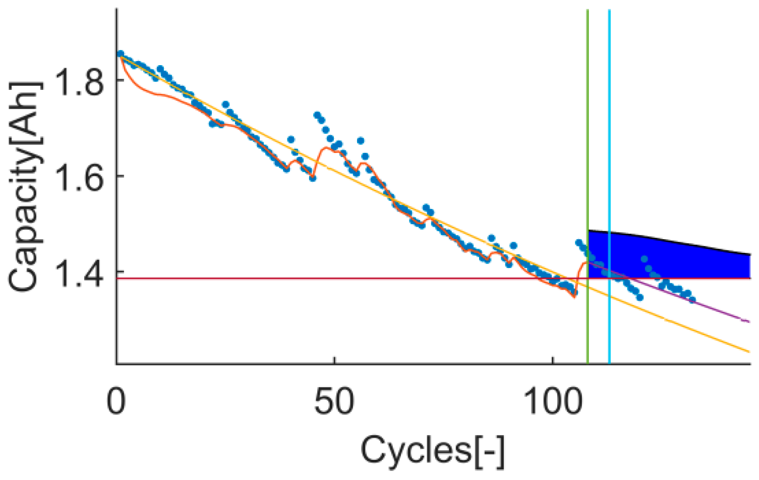
Figure 2.
An example of the trial-instant figure with a training data set of 71 samples from which the last 6 samples compose the validation data set (the vertical green line represents the learning threshold, and the blue line represents the training threshold). The prior knowledge is composed by a linear model (yellow line) and data from the battery B0007 (blue dots). The time-instant of interest is defined by the EOL threshold (the horizontal red line), which is the capacity value at the 146 sample. The prediction probability density is displayed by the green area called PDF. The algorithm response on the learning data set is the orange line. The purple line represents the algorithm response on the rest of the data set.

Figure 3.
The input data with low uncertainty.

Figure 4.
The input data with high uncertainty.

Figure 5.
Results from test nº 1 (“B0007” linearly modelled).

Figure 6.
Results from test nº 2 (“B0018” linearly modelled).

Figure 7.
Results from test nº 3 (“B0007” modelled with a double exponential).

Figure 8.
Results from test nº 4 (“B0018” modelled with a double exponential).

Figure 9.
Time-instant figure of test 1 on t4.

Figure 10.
Time-instant figure of test 3 on t4.

Figure 11.
Time-instant figure of test 1 on t11.

Figure 12.
Time-instant figure of test 3 on t11.

Figure 13.
Time-instant figure of test 1 on t17.

Figure 14.
Time-instant figure of test 3 on t17.

Figure 15.
Time-instant figure of test 1 on t65.

Figure 16.
Time-instant figure of test 3 on t65.

Figure 17.
Time-instant figure of test 1 on t118.

Figure 18.
Time-instant figure of test 3 on t118.

Figure 19.
Time-instant figure of test 2 on t1.

Figure 20.
Time-instant figure of test 4 on t1.

Figure 21.
Time-instant figure of test 2 on t38.

Figure 22.
Time-instant figure of test 4 on t38.

Figure 23.
Time-instant figure of test 2 on t55.

Figure 24.
Time-instant figure of test 4 on t55.

Figure 25.
Time-instant figure of test 2 on t78.

Figure 26.
Time-instant figure of test 4 on t78.

Figure 27.
Time-instant figure of test 2 on t102.

Figure 28.
Time-instant figure of test 4 on t102.


Table 1.
Set of metrics that quantifies the correctness.
| Metric | Description |
|---|---|
| RMSE | Root Mean Squared Error (RMSE) on the known prediction data set (prediction fitting error) [8,34]. |
| RA | Relative Accuracy (RA) of the predicted RUL respect to the real RUL [18]. |
| Pvalue | The probability of estimating the ground truth (from a normalized Probability Distribution Function (PDF)) [36]. |
| Pwidth | The relative width of the probability distribution with a 68% confidence range respect to the real RUL [24]. |
Table 2.
Set of metrics that quantifies the timeliness.
| Metric | Description |
|---|---|
| PH | The Prognosis Horizon (PH) defines from which time-instant of interest the accuracy of the algorithm reaches a certain threshold β (minimum acceptable probability mass) [18]. |
| CRA | The convergence of the relative accuracy (CRA) quantifies the rate at which the RA improves with time [18]. |
Table 3.
Set of metrics that quantifies the computational performance.
| Metric | Description |
|---|---|
| FLOP counts | The number of operations executed in an algorithm computed by Floating-point operations (FLOP) [3]. |
Table 4.
Reference values of the unified set of metrics.
| Metrics | “Worst” | “Best” |
|---|---|---|
| Prediction RMSE | ∞ | 0 |
| RA | −∞ | 1 |
| Pvalue | 0 | 1 |
| Pwidth | ∞ or 0 | Between 0 and 1 |
| PH | 0 | 1 |
| CRA | ∞ | 0 |
| FLOP counts | ∞ | 0 |
Table 5.
Proposed trial matrix to separate input uncertainty effect on algorithm’s evaluation.
| Cases | Data | “Best” | ||
|---|---|---|---|---|
| Low Uncertainty | High Uncertainty | Low Uncertainty | High Uncertainty | |
| 1 | X | X | ||
| 2 | X | X | ||
| 3 | X | X | ||
| 4 | X | X | ||
Table 6.
Trials of the stochastic tools.
| Test n | Stochastic Tool | Aging Model | Cell |
|---|---|---|---|
| 1 | Particle FIlter | Equation (11) | “B0007” |
| 2 | “B0018” | ||
| 3 | Equation (12) | “B0007” | |
| 4 | “B0018” |
Table 7.
Affecting parameters.
| Parameters | Value | Description |
|---|---|---|
| Tmin | 10% | Minimum training data set (). |
| 50% | The minimum acceptable probability mass [26]. | |
| 5% | The relative error [23]. | |
| 500 | Particle quantity [50]. | |
| L | 4% | Validation data set. |
| EOL | 7/8 | End-of-Life time-instant situation on the data set. |
| Cv | 10 | Running times at parameterization. |
| NT | 50 | Resampling threshold % respect to the particle quantity. |
| 1 | The delta time-instant from one time-instant to the next one. |
Table 8.
Hyper-parameters.
| Metric | Description |
|---|---|
| The variance of the state model’s Gaussian noise. | |
| The variance of the observation model’s Gaussian noise. | |
| The variance of the initial Gaussian distribution of the particles. |
Table 9.
Grid Search Optimization grid.
| Parameters | High Limit | Intervals | Low Limit |
|---|---|---|---|
| 1.5 | 0.6, 0.1, 0.05, 0.02, 0.01, 0.005, 0.002, 0.001 | 0.0005 | |
| 1.5 | 0.6, 0.1, 0.05, 0.02, 0.01, 0.005, 0.002, 0.001 | 0.0005 | |
| 0.1 | 0.05 | 0.01 |
Table 10.
The PH, CRA and the number of FLOPs on all the tests.
| Test | PH | CRA | FLOP Counts |
|---|---|---|---|
| 1 | 0.8702 | 58.9247 | 2,379,860 |
| 2 | 1 | 8.1662 | 1,869,890 |
| 3 | 0.9313 | 64.5086 | 5,459,580 |
| 4 | 1 | 4.2028 | 4,289,670 |
Table 11.
The RMSE, RA, Pvalue and Pwidth of 5 time-instant of interest on tests 1 (B0007 and linear equation).
Table 11.
The RMSE, RA, Pvalue and Pwidth of 5 time-instant of interest on tests 1 (B0007 and linear equation).
| Prediction-Time-Instant | Prediction RMSE | RA | ||
|---|---|---|---|---|
| 4 | 0.0650 | 0.8425 | 0.60 | 0.57 |
| 11 | 0.0262 | 0.9917 | 0.92 | 0.04 |
| 17 | 0.0443 | 0.8596 | 0 | 0.04 |
| 65 | 0.0340 | 0.8788 | 0.06 | 0.04 |
| 118 | 0.0246 | 0.9231 | 0.95 | 0.03 |
Table 12.
The RMSE, RA, Pvalue and Pwidth of 5 time-instant of interest on tests 3 (B0007 and exponential equation).
Table 12.
The RMSE, RA, Pvalue and Pwidth of 5 time-instant of interest on tests 3 (B0007 and exponential equation).
| Prediction-Time-Instant | Prediction RMSE | RA | ||
|---|---|---|---|---|
| 4 | 0.0355 | 0.9685 | 0.81 | 0.07 |
| 11 | 0.0215 | 0.9333 | 0.62 | 0.50 |
| 17 | 0.0210 | 0.9912 | 0.75 | 1.78 |
| 65 | 0.0260 | 0.9242 | 0.85 | 0.18 |
| 118 | 0.0173 | 0.9231 | 0.81 | 0.03 |
Table 13.
The RMSE, RA, Pvalue and Pwidth of 5 time-instant of interest on tests 2 (B0018 and linear).
Table 13.
The RMSE, RA, Pvalue and Pwidth of 5 time-instant of interest on tests 2 (B0018 and linear).
| Prediction-Time-Instant | Prediction RMSE | RA | ||
|---|---|---|---|---|
| 1 | 0.0368 | 0.9417 | 0.64 | 0.93 |
| 38 | 0.0742 | 0.6667 | 0 | 0.01 |
| 55 | 0.0707 | 0.5918 | 0.59 | 0.66 |
| 78 | 0.0921 | 0.1538 | 0.02 | 0.31 |
| 102 | 0.0198 | −0.5000 | 0.93 | 0.94 |
Table 14.
The RMSE, RA, Pvalue and Pwidth of 5 time-instant of interest on tests 4 (B0018 and exponential equation).
Table 14.
The RMSE, RA, Pvalue and Pwidth of 5 time-instant of interest on tests 4 (B0018 and exponential equation).
| Prediction-Time-Instant | Prediction RMSE | RA | ||
|---|---|---|---|---|
| 1 | 0.0425 | 0.9417 | 0.89 | 0.34 |
| 38 | 0.2936 | 0.3333 | 0 | 0.28 |
| 55 | 0.0911 | 0.5306 | 0.43 | 1.02 |
| 78 | 0.1101 | 0.1538 | 0 | 0.01 |
| 102 | 0.0219 | −2.5000 | 0.04 | 0.01 |
Publisher’s Note: MDPI stays neutral with regard to jurisdictional claims in published maps and institutional affiliations. |
© 2021 by the authors. Licensee MDPI, Basel, Switzerland. This article is an open access article distributed under the terms and conditions of the Creative Commons Attribution (CC BY) license (https://creativecommons.org/licenses/by/4.0/).
Share and Cite
MDPI and ACS Style
Arrinda, M.; Oyarbide, M.; Macicior, H.; Muxika, E. Unified Evaluation Framework for Stochastic Algorithms Applied to Remaining Useful Life Prognosis Problems. Batteries 2021, 7, 35. https://0-doi-org.brum.beds.ac.uk/10.3390/batteries7020035
AMA Style
Arrinda M, Oyarbide M, Macicior H, Muxika E. Unified Evaluation Framework for Stochastic Algorithms Applied to Remaining Useful Life Prognosis Problems. Batteries. 2021; 7(2):35. https://0-doi-org.brum.beds.ac.uk/10.3390/batteries7020035
Chicago/Turabian StyleArrinda, Mikel, Mikel Oyarbide, Haritz Macicior, and Eñaut Muxika. 2021. "Unified Evaluation Framework for Stochastic Algorithms Applied to Remaining Useful Life Prognosis Problems" Batteries 7, no. 2: 35. https://0-doi-org.brum.beds.ac.uk/10.3390/batteries7020035
Note that from the first issue of 2016, this journal uses article numbers instead of page numbers. See further details here.