Analysis of Electrochemical Impedance Spectroscopy on Zinc-Air Batteries Using the Distribution of Relaxation Times

Abstract

Zinc-air batteries could be a key technology for higher energy densities of electrochemical energy storage systems. Many questions remain unanswered, however, and new methods for analyses and quantifications are needed. In this study, the distribution of relaxation times (DRT) based on ridge regression was applied to the impedance data of primary zinc-air batteries in a temperature range of 253 K and 313 K and at different State-of-Charges for the first time. Furthermore, the problem of the regularization parameter on real impedance spectroscopic measurements was addressed and a method was presented using the reconstruction of impedance data from the DRT as a quality criterion. The DRT was able to identify a so far undiscussed process and thus explain why some equivalent circuit models may fail.

1. Introduction

The restructuring of electrical energy production to renewable energies is accompanied by a volatile energy generation and requires energy storage in order to regulate production and demand. In the field of electrochemical energy storage, lithium-ion batteries (LIBs) are probably the best-known electrical energy storage technologies [1], but they have significant shortcomings in terms of cost, safety, and specific capacity. Zinc-air batteries (ZABs), for example, are comparatively cheaper, safer, and have a three times higher theoretical gravimetric capacity of about 820 Ah kg${}^{-1}$ based on the active material compared to an LiCoO${}_2$ LIB. The reason is mainly due to the working principle of ZABs, as two electrons are moved per mass transfer and the required oxygen is extracted from the ambient air. Despite the principle rechargeability of the technology, ZABs exist commercially only as primary batteries and are used mainly in hearing aids [2]. A suitable electrocatalyst for both an efficient oxygen reduction reaction (ORR) and an oxygen evolution reaction (OER) cycle has not yet been found [3,4,5], nor has a filter that regulates the oxygen and the humidity from the ambient air been developed [6,7]. The dendrite growth [8,9,10,11], the shape change [12,13,14], the passivation of the anode [15,16,17,18] and the zincate transport into the gas diffusion layer (GDL) during charging [19] are also critical parameters for rechargeability. In order to prevent such processes, it is necessary to gain a fundamental understanding of the reactions and their interactions [20]. One common method for this is the electrochemical impedance spectroscopy (EIS) [21], which is used for material optimization and modeling besides process analysis and quantification [22,23,24,25,26,27,28,29]. In addition to the visual evaluation of the impedance data, fitted equivalent circuit models (ECM) are used for quantification [21]. However, different combinations of equivalent circuit elements can produce the same results [30], which can lead to misinterpretations [31], especially if the type and the number of the involved processes are not clearly determined. Furthermore, the separation and the readability are hardly given for similar or overlapping processes, e.g., the negative electrode is similar to the positive electrode in character, then the time constants of both electrodes can influence the same measuring points in the frequency range. Therefore, the interpretation of the impedance data using the universal distribution of relaxation times (DRT) approach is becoming increasingly popular [32,33,34,35,36,37,38,39], since no deeper prior knowledge of chemical-physical or electrical models is required and superimposed processes can possibly be distinguished.

In this article, the DRT was applied to commercial zinc-air primary cells for the first time. For this purpose, the primary cells were measured by EIS at temperatures between 253 K and 313 K and different States-of-Charges (SoCs). The SoCs were targeted by four different discharge currents during the galvanostatic discharge. In addition to the process analysis, the capacity of the primary ZABs was also discussed. Furthermore, the Gaussian probability distribution function was presented for the quantification of the individual processes, which were identified from the DRT. For the determination of the regularization parameter, used in the ridge regression for solving the DRT, a method was implemented to compare the reconstructed spectrum with the EIS measurement. The use of a brute force algorithm coupled with a minimization algorithm provided reliable values. The issue of varying the regularization parameter was also critically discussed in this study.

2. Materials and Methods

2.1. Electrochemical Impedance Spectroscopy

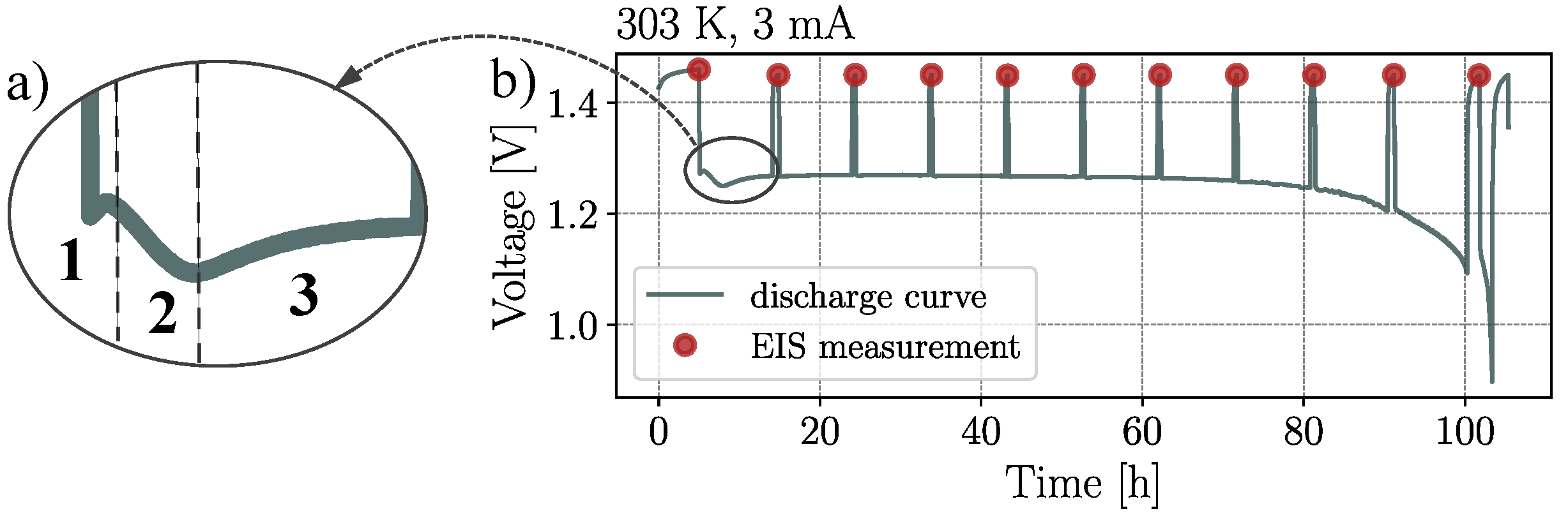
The EIS measurements were performed on commercial ZABs of the type PR48 with a nominal capacity of about 300 mAh. For one experiment, 4 cells from a blister were used for the characterization and 2 cells were used for preliminary studies, where the capacity was determined (see

Table 1. Measured capacities depending on discharge current and ambient temperature.

Current	253 K	263 K	273 K	283 K	294 K	303 K	313 K
3 mA	39 mAh	43 mAh	202 mAh	257 mAh	254 mAh	275 mAh	287 mAh
4 mA	-	-	188 mAh	231 mAh	232 mAh	246 mAh	287 mAh
5 mA	-	-	108 mAh	211 mAh	221 mAh	239 mAh	261 mAh
6 mA	-	-	89 mAh	187 mAh	215 mAh	220 mAh	260 mAh

) by using a constant discharge current (applied by a Neware BTS5V10mA potentiostat) in a climate chamber (Binder MK 56) related to the defined current and the temperature combinations. The primary investigation includes the combination of the temperatures of 273, 283, 294, 303, and 313 K with 3, 4, 5, and 6 mA discharge currents, respectively. For the current of 3 mA, the temperatures of 253 K and 263 K were also examined. The cells were connected to a custom four-wire measurement holder and were measured with a PARSTAT^® MC PMC-2000A potentiostat/galvanostat. First, the cells were unsealed and rested at least for 5 h at a defined temperature until they reached the open cell voltage (OCV) of 1.45 V. Then, 10% SoC was gradually discharged from the cells and after resting up to 1.45 V, a galvanostatic EIS was performed. This procedure was repeated until a cut-off voltage of 0.9 V was reached and is shown in Figure 1. The EIS measurement was carried out between 50 mHz and 1.75 MHz with a current amplitude of $A_{\mathrm{RMS}}=$ 1.5 mA and a superimposed discharge DC current of 3 mA. A total of 10 values per decade were recorded and the average of 3 consecutive cycles was taken, resulting in an SoC change of less than 0.15%. In an additional study for investigating the inhomogeneous discharge behavior during the first 10% SoC discharge, as shown in (Figure 1a), the frequency range of the EIS measurement was reduced to 10 Hz and 1 MHz, which decreased the measurement time from about 7.5 min to 20 s. Contrary to the routine described above, the cells were only discharged by the superimposed DC current of the EIS measurement, which was repeated permanently.

2.2. Distribution of Relaxation Times

The basic idea of the DRT is the approximation of the measured data by an infinite series of overlapping resistor and capacitor (RC) circuits in parallel form. The weighting of the individual terms is described by a distribution function:

$$Z_{\mathrm{DRT}}\left(\omega \right)=R_{\infty }+\underset{0}{\overset{\infty }{\int }}\frac{h\left(\tau \right)}{1+\mathrm{j}\omega \tau }\mathrm{d}\tau .$$

(1)

Normalizing the distribution function to the total polarization of the system yields the more common representation of the DRT:

$$Z_{\mathrm{DRT}}\left(\omega \right)=R_{\infty }+R_{\mathrm{p}}\underset{0}{\overset{\infty }{\int }}\frac{g\left(\tau \right)}{1+\mathrm{j}\omega \tau }\mathrm{d}\tau .$$

(2)

The solution of the distribution function $g\left(\tau \right)$ corresponds to a deconvolution in the frequency domain. However, as the distribution function is not uniquely defined, various approaches including the Fourier transform [34,40,41], Bayesian methods [38,42,43,44,45], Monte Carlo algorithms [46,47,48], genetic algorithms [49,50], and regression methods [35,37,39,51,52,53,54,55,56] have been developed. The numerical method, used in this paper to solve the distribution function, makes use of a discretization of the integral term:

$$Z_{\mathrm{DRT}}\left(\omega \right)=\sum _{k=1}^n\frac{h_k}{1+\mathrm{j}\omega {\tau }_k}=R_{\mathrm{p}}·\sum _{k=1}^n\frac{g_k}{1+\mathrm{j}\omega {\tau }_k}.$$

(3)

If the number of integration steps is set to one, the impedance description of an RC element is obtained:

$$Z_{\mathrm{RC}}\left(\omega \right)=\frac{R}{1+\mathrm{j}\omega {\tau }_{\mathrm{RC}}},$$

(4)

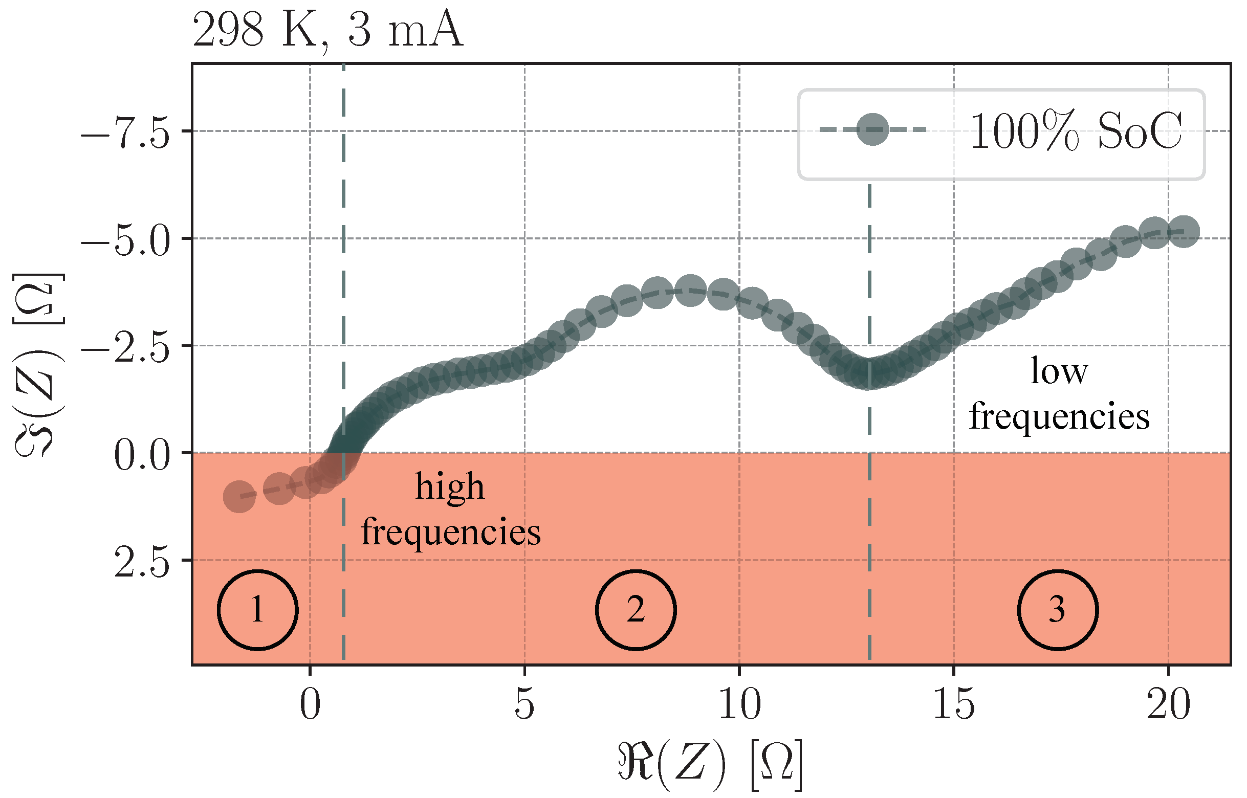
where $\tau =RC=\frac{1}{\omega }$ and $g_k=\frac{R}{R_{\mathrm{P}}}$. If the impedance data represents exactly one RC element, then with $n=1$ the Equation (3) would be well defined and the distribution function would be a peak at a fixed time constant. For $n=2$ it can be recognized that the Equation (3) is ill-posed, since both the first and the second RC element would be able to map a perfect semicircle. Thus, the number of iteration steps $[{\tau }_1,\dots ,{\tau }_n]$ has a critical influence on the quality of the distribution function (illustrated in Figure A1). As long as the interval is identical to the number of measuring points, it is guaranteed that for each measuring point an RC element with corresponding threshold frequency exists. Since the DRT is ohmic-capacitive, no inductive components can be considered and it is assumed:

$$\Im \left\{Z\left(\omega \right)\right\}\stackrel{!}{\le }0\forall \omega .$$

(5)

Thus, there is a limited range for the applicability of the DRT to the impedance data as shown in Figure 2. An approach to consider also inductive elements was presented by Danzer adding an ohmic-inductive term to the DRT [37]. Nevertheless, by a boundary analysis, the imaginary part of an RC elements normally follows:

$$\begin{array}{c}\hfill \underset{\omega \to 0}{lim}\Im \left\{Z\left(\omega \right)\right\}\stackrel{!}{=}0,\end{array}$$

(6)

$$\begin{array}{c}\hfill \underset{\omega \to \infty }{lim}\Im \left\{Z\left(\omega \right)\right\}\stackrel{!}{=}0.\end{array}$$

(7)

For example, if the measurement does not converge against the real axis due to a dominant diffusion process at low frequencies as shown in Figure 2, the associated RC elements can become very large and thus overshadows the entire DRT (see Figure 3b).

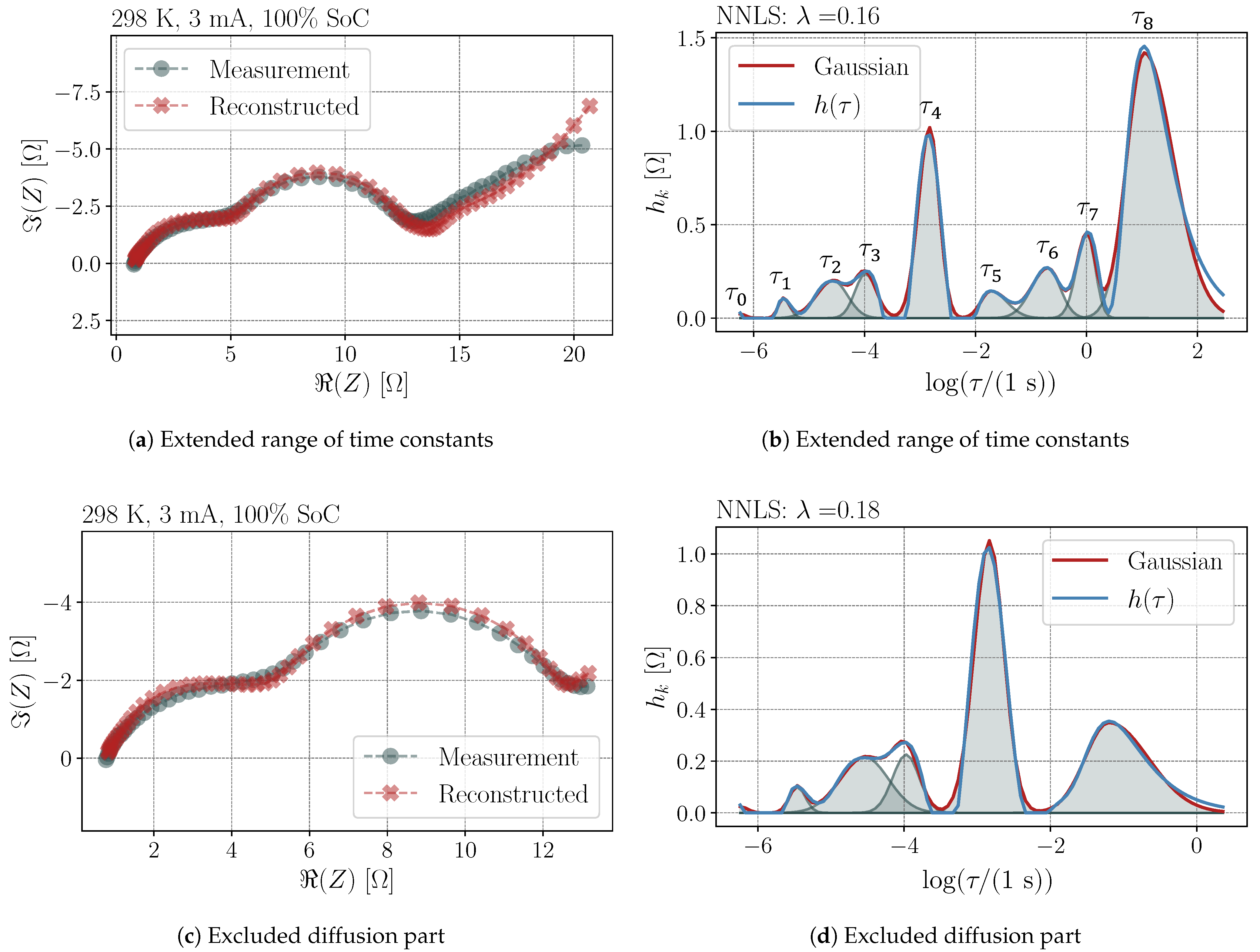
Hahn et al. propose to extend the interval of the specified time constants beyond the limits of the measurement frequencies, which is usually given by ${\tau }_{\min }=\frac{1}{2\pi f_{\max }}$ to ${\tau }_{\max }=\frac{1}{2\pi f_{\min }}$ [35]. It is also possible to exclude the diffusion part from the consideration of the DRT and analyze it through other methods [57]. Figure A2 validates the practicality for extending the time constants for low frequencies as well as for excluding the diffusion part. Finally, the DRT can be seen as a minimization problem between measurement ${\mathbf{Z}}_{\mathrm{Meas}}$ and ${\mathbf{Z}}_{\mathrm{DRT}}$ (cf. Equation (3)):

$$\min \left\{{\parallel {\mathbf{Z}}_{\mathrm{Meas}}-{\mathbf{Z}}_{\mathrm{DRT}}\parallel }_2^2\right\}.$$

(8)

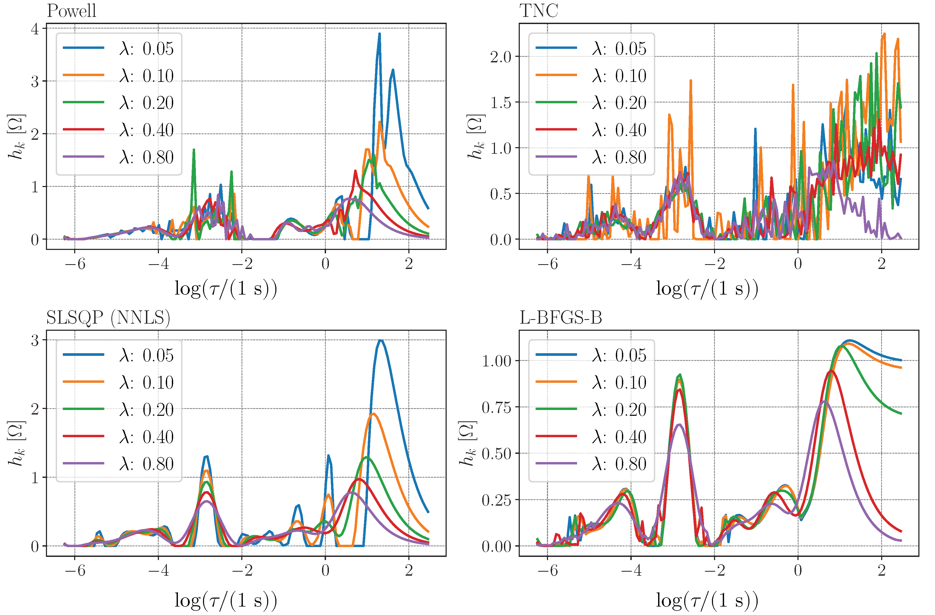
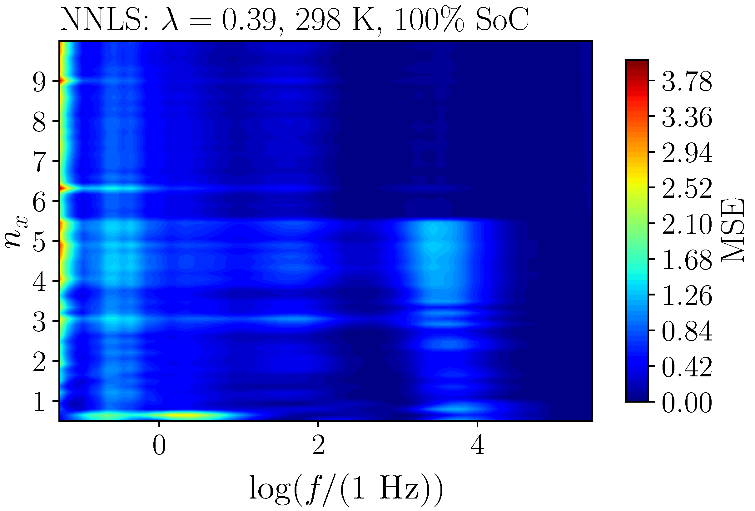
To solve this problem, only the non-negative least squares (NNLS) [58] and the complex non-linear least squares algorithm (CNLS) [59] are mentioned in the literature. In this study, other existing algorithms with boundary conditions (Powell, TNC, SLSQP, L-BFGS-B) from the Optimization Toolbox of SciPy were evaluated (depicted in Figure 4), with the result that only the NNLS, the sequential least squares programming algorithm (SLSQP) [60], which is a slight modification of the NNLS algorithm, and the L-BFGS-B algorithm [61] provide feasible results.

Therefore, the following equations refer only to the NNLS algorithm to ensure comparability within the literature. The NNLS algorithm solves the problem by matrix and vector operations. The Equation (3) becomes a normalized matrix entry:

$$A_{i,k}=\frac{1}{1+\mathrm{j}{\omega }_i{\tau }_k},$$

(9)

with $\{i\in \mathbb{N}\mid 0<i\le m\}$ and $\{k\in \mathbb{N}\mid 0<k\le n\}$. The measurement data is defined as a vector $\mathit{b}$ with m measurement points. Since the measured values are given as complex numbers, which is not supported by the NNLS algorithm, the DRT can be calculated from the real and the imaginary part:

$$\mathit{A}=\left[\begin{array}{ccc}\Re \{A_1,1\}& \cdots & \Re \left\{A_{1,n}\right\}\\ ⋮& \ddots & ⋮\\ \Re \left\{A_{m,1}\right\}& \cdots & \Re \left\{A_{m,n}\right\}\\ \Im \{A_1,1\}& \cdots & \Im \left\{A_{1,n}\right\}\\ ⋮& \ddots & ⋮\\ \Im \left\{A_{m,1}\right\}& \cdots & \Im \left\{A_{m,n}\right\}\end{array}\right],\mathit{b}=\left[\begin{array}{c}\Re \{Z_{\mathrm{Meas}},1\}\\ ⋮\\ \Re \left\{Z_{\mathrm{Meas},m}\right\}\\ \Im \{Z_{\mathrm{Meas}},1\}\\ ⋮\\ \Im \left\{Z_{\mathrm{Meas},m}\right\}\end{array}\right].$$

(10)

The distribution function is also specified as a vector $\mathit{x}$ with the constraint:

$$x_k=g_k\ge 0\forall k\in \mathbb{N}\mid 0<k\le n.$$

(11)

In the case that the solution of the minimization problem is an ill-posed problem, since the data may be noisy or the sampling frequency is higher than the measurement frequency, a regularization term according to Tikhonov et al. can be added to the Equation (8) in matrix notation [62]:

$$\min \left\{{\parallel \mathit{A}\mathit{x}-\mathit{b}\parallel }_2^2+{\lambda }_{\mathrm{DRT}}{\parallel \mathit{M}\mathit{x}\parallel }_2^2\right\}.$$

(12)

If the regularization matrix is simplified by the identity matrix, the ridge regression with the regularization parameter ${\lambda }_{\mathrm{DRT}}$ is obtained.

2.3. Determination of the Regularization Parameter

The determination of the regularization parameter for the ridge regression is the current state of research and leads to different approaches [39,51,55,63]. Without regularization, the DRT would tend to oscillate, but excessive values for $\lambda$ can suppress characteristic peaks (see Figure 4). Hahn et al. have examined the common methods (Discrepancy, Cross-Validation, and L-Curve) and have found them to be unsatisfactory [35]. They have proposed the solution using the residual sum of squares as a quality parameter. Based on this idea, a modified approach was used here that uses the Nelder–Mead method to optimize the regularization parameter so that the error between measurement and reconstructed spectrum of DRT after post-processing (see Section 2.4) becomes minimal:

$$\min \left\{\frac{1}{m}\sum _{i=1}^m\mid Z_{\mathrm{Meas},i}-Z_{\mathrm{DRT},i}\left({\lambda }_{\mathrm{DRT}}\right)\mid \right\}.$$

(13)

Since this approach quickly converges to a local minimum and thus the determination of the parameter strongly depends on the initial condition, the regularization parameter was estimated via a brute-force algorithm by variation of $\{{\lambda }_{\mathrm{DRT}}\in \mathbb{R}\mid 0\le {\lambda }_{\mathrm{DRT}}\le 1\}$ in advance. This method has proven to be very reliable for reconstruction of the measured impedance data.

2.4. Preparation of DRT for Electrochemical Analysis

With only the determination of $h_k$, it is possible to identify the number of chemical-physical processes and to observe the change of the DRT, e.g., via charging and discharging or aging [64]. However, quantitative statements about the individual processes are not feasible. Since the DRT already represents the sum of RC elements, it is obvious to describe the processes by an equivalent circuit based on RC elements, provided that the system is well known, in order to reasonably limit the number of RC elements [65]. Moreover, not every process can be described by a limited number of RC elements [65]. Another idea is to consider the DRT not as a sum of RC elements, but as a function, which in turn can be approximated by arbitrary functions depending on physical processes [30]. The superposition of these processes, on the other hand, maps the DRT:

$$g_{\mathrm{DRT}}\left(\tau \right)=\sum _{j=1}^N{g}_{\mathrm{Peak},j}\left(\tau \right).$$

(14)

Since the solution of the DRT already provides a broad distribution of the relaxation times, it is obvious to describe the individual processes by a Gaussian probability distribution function [35,41,44,49,50]:

$$g_{\mathrm{Peak},j}=a_{0,j}·exp\left\{-\frac{1}{2}{\left(\frac{{log}_{10}(\tau /{\tau }_{\mathrm{p},j})·(1+s_j·\mathrm{sgn}\left({log}_{10}(\tau /{\tau }_{\mathrm{p},j})\right)}{{\sigma }_j}\right)}^2\right\}.$$

(15)

The modified Gaussian distribution, here, includes the prefactor $a_{0,j}$, which adjusts the height of the Gaussian curve at the expected value ${\tau }_{\mathrm{p},j}$. The variance ${\sigma }_j^2$ determines the width of the probability distribution function and the skewness $s_j$ describes the asymmetry. Wide or skewed distributions could indicate non-ideal processes, inhomogeneities, side reactions, or errors in the measurement.

3. Results

3.1. Regularization

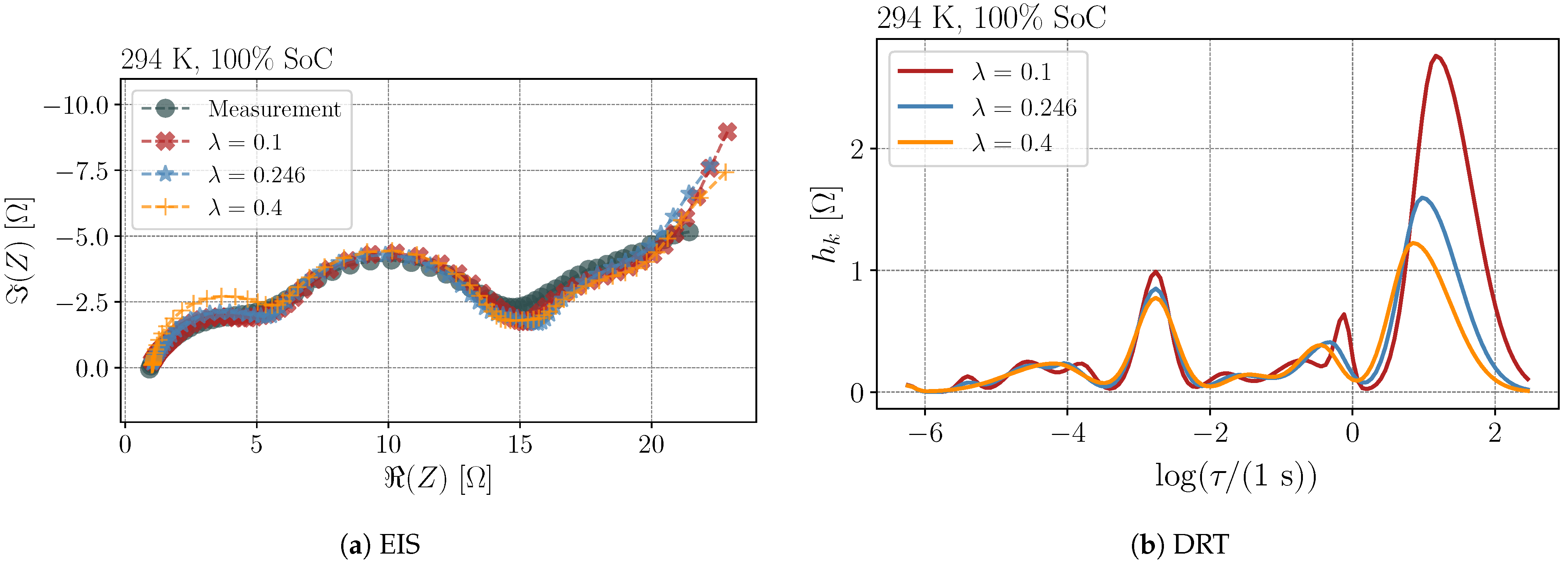
The determination of the regularization parameter $\lambda$, using the proposed routine, was performed for each measured data set. The results are shown in Figure 5. It was demonstrated that, depending on the SoC, the temperature and the currents used, large deviations arose in the determination of a suitable regularization parameter. Especially at the higher temperatures, the range for $\lambda$ extended from about 0.05 to 0.7, while the median of all data sets varied between approximately 0.05 and 0.2. Besides the already discussed number of time constants and the extension of the time domain, large deviation occurred due to the strong change of the impedance spectra between 100% SoC and 90% SoC on the one hand and on the other hand to the erroneous approximation of the diffusion part by a limited number of RC elements. Figure A3 shows the comparison between an optimal ($\lambda =0.246$), a lower ($\lambda =0.1$) and a higher ($\lambda =0.4$) regularization parameter for the measured impedance spectrum at 294 K and 100% SoC. Lower values lead to more peaks and correspondingly to additional RC elements, which in principle improves the reconstruction of the measurement; however, the physical interpretation of the DRT becomes more and more impossible. Higher values smooth out smaller peaks, resulting in fewer RC elements, greatly simplifying the reconstruction and possibly leaving small hidden processes in the DRT undetected. Thus, the most significant discrepancy in finding an appropriate regularization parameter is less the method and more the result for interpreting the data. According to the high deviation and the associated change in DRT as well as the physical significance, the variation of the regularization parameter within a technology is not meaningful. Consequently, for all further investigations, the upper median of $\lambda =0.2$ was set for this parameter.

3.2. Temperatures and Currents

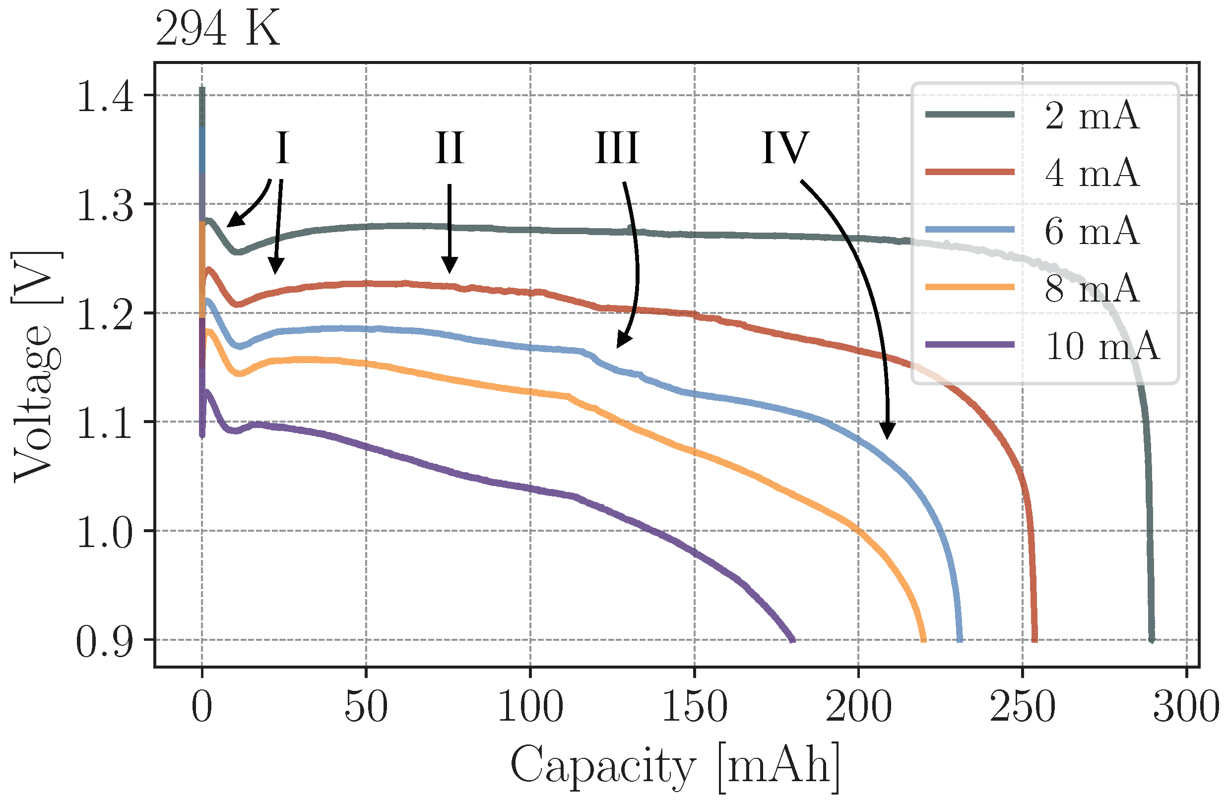
The discharge profiles at different currents, i.e., between 2 mA and 10 mA, are shown in Figure 6. The investigated cells had a diameter of 7.8 mm, resulting in current densities of about 42 Am${}^{-2}$ to 210 Am${}^{-2}$. The voltage profiles and the capacities were diminished with increasing discharge currents. Four different operating phases could be identified through the analysis of the discharge profiles related to the applied currents:

I

As shown in Figure 1, the initial operating phase could be subdivided into three specific processes. The process I.1 was very fast and has slightly recovered the voltage in respect of the initial voltage drop. This was followed by process I.2, which resulted in a linear decrease of the voltage until a minimum was reached. In process I.3 the voltage gradually recovered and converged to a constant value. All three processes occurred independently of the current, with process I.1 and I.2 also appearing to be time independent.

II

The corresponding capacity in the nearly constant voltage operating phase II was depended on the the applied discharge currents, i.e., the greater the discharge current, the smaller the duration.

III

After the constant operating phase for currents greater than 4 mA, an additional voltage drop was observable. Especially between 4 mA and 8 mA this phase is clearly detectable.

IV

In the final operating phase, the voltage decreased rapidly until it reached the cut-off voltage. As the current increased, the boundary between phase III and IV became unclear.

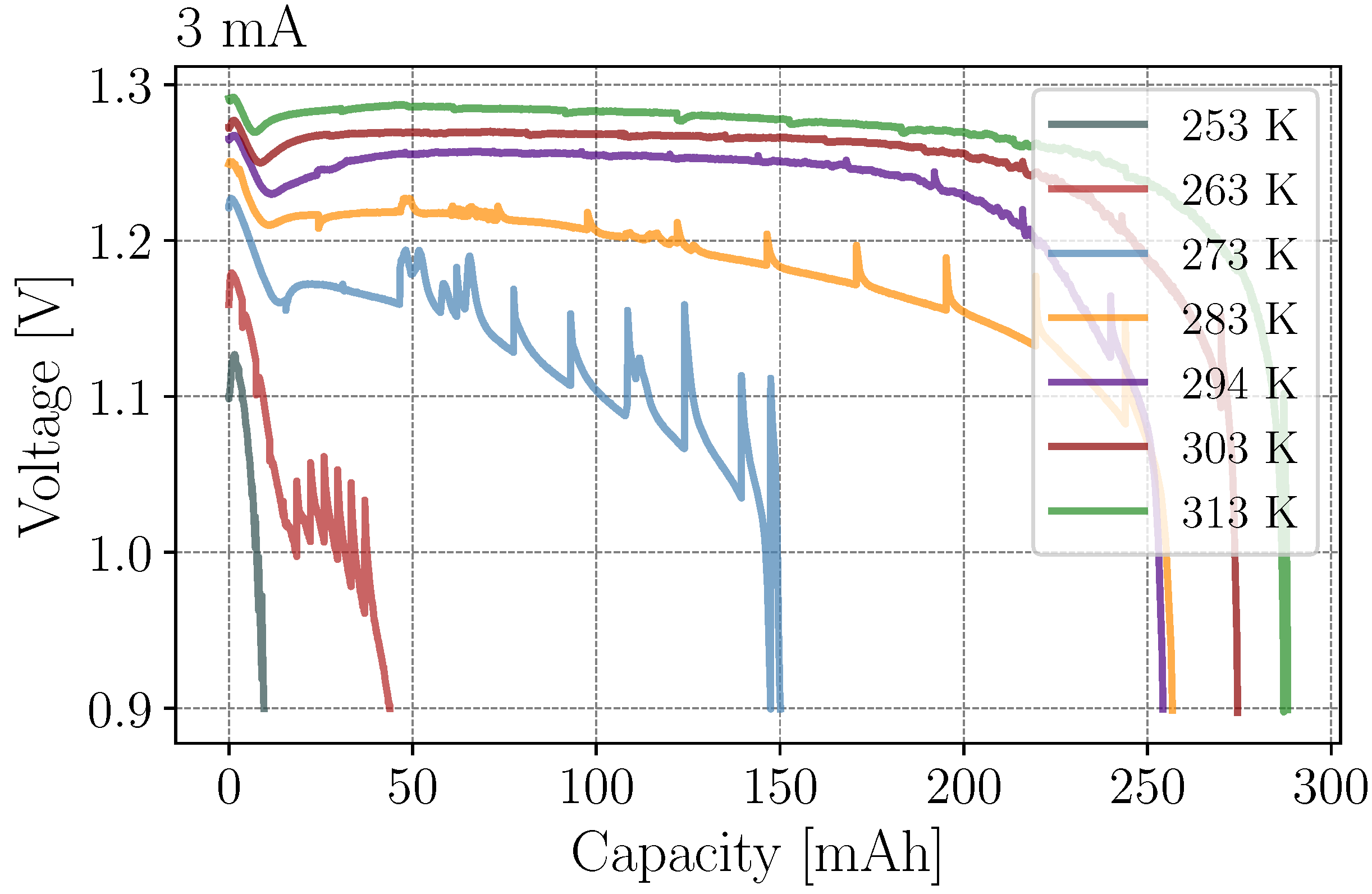
Figure 6 shows a strong dependence of the discharge capacity on the applied discharge currents. The capacities were measured as a function of current and temperature in order to target the corresponding SoC values, and are presented in Table 1. The values indicate that the maximum available capacity was diminished by both high currents and low temperatures. Especially at currents higher than 3 mA and temperatures below 273 K, it was not possible to determine the capacity via a constant current discharge. The dependence of the temperature is depicted in Figure A4.

3.3. Process Analysis

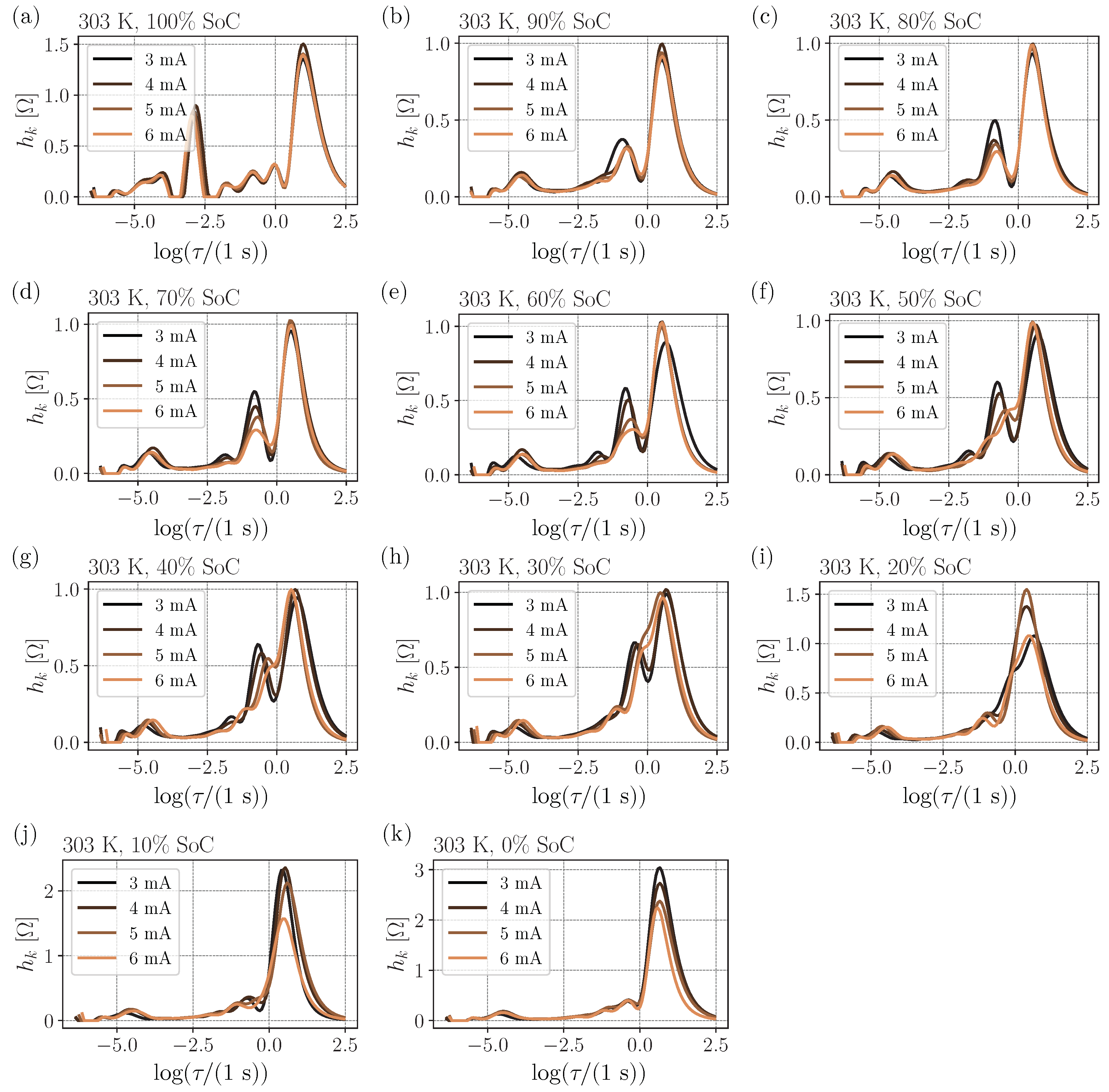
The DRT is intended for identifying and quantifying chemical-physical processes from impedance data without extensive model fitting. For the proof of concept of the DRT, the data set at 303 K was selected because it yielded the smallest variation in the mean value of the regularization parameter with respect to the current. With a regularization parameter of $\lambda =0.2$, eight peaks were found for all currents at an SoC of 100% (see Figure 7a, cf. Figure A2b). The corresponding time constant ${\tau }_0$ from

Table 2. Time constants and height of the characteristic peaks depending on the SoC at 303 K and a discharge current of 3 mA.

SoC in %	$log\left({\mathit{\tau }}_0\right)$	$log\left({\mathit{\tau }}_1\right)$	$log\left({\mathit{\tau }}_2\right)$	$log\left({\mathit{\tau }}_3\right)$	$log\left({\mathit{\tau }}_4\right)$	$log\left({\mathit{\tau }}_5\right)$	$log\left({\mathit{\tau }}_6\right)$	$log\left({\mathit{\tau }}_7\right)$	$log\left({\mathit{\tau }}_8\right)$
100	4.6 × ${10}^{-7}$	2.5 × ${10}^{-6}$	1.9 × ${10}^{-5}$	9.8 × ${10}^{-5}$	1.2 × ${10}^{-3}$	1.7 × ${10}^{-2}$	1.6 × ${10}^{-1}$	9.2 × ${10}^{-1}$	9.7
90.2	4.6 × ${10}^{-7}$	3.1 × ${10}^{-6}$	2.5 × ${10}^{-5}$	-	-	9.2 × ${10}^{-3}$	1.3 × ${10}^{-1}$	-	3.4
80.3	4.6 × ${10}^{-7}$	3.1 × ${10}^{-6}$	2.1 × ${10}^{-5}$	-	-	1.2 × ${10}^{-2}$	1.5 × ${10}^{-1}$	-	3.4
70.5	4.6 × ${10}^{-7}$	3.1 × ${10}^{-6}$	2.5 × ${10}^{-5}$	-	-	1.4 × ${10}^{-2}$	1.5 × ${10}^{-1}$	-	3.4
60.7	4.6 × ${10}^{-7}$	2.7 × ${10}^{-6}$	1.8 × ${10}^{-5}$	3.5 × ${10}^{-4}$	-	1.7 × ${10}^{-2}$	1.5 × ${10}^{-1}$	-	4.6
50.5	4.6 × ${10}^{-7}$	2.7 × ${10}^{-6}$	1.6 × ${10}^{-5}$	3.1 × ${10}^{-4}$	-	1.7 × ${10}^{-2}$	1.8 × ${10}^{-1}$	-	5.3
41.0	4.6 × ${10}^{-7}$	2.7 × ${10}^{-6}$	1.6 × ${10}^{-5}$	-	-	2.2 × ${10}^{-2}$	2.0 × ${10}^{-1}$	-	5.3
31.1	4.6 × ${10}^{-7}$	2.7 × ${10}^{-6}$	1.6 × ${10}^{-5}$	2.0 × ${10}^{-4}$	-	-	3.7 × ${10}^{-1}$	-	4.6
21.3	4.6 × ${10}^{-7}$	2.7 × ${10}^{-6}$	1.6 × ${10}^{-5}$	1.1 × ${10}^{-4}$	-	-	-	-	4.6
11.5	4.6 × ${10}^{-7}$	3.1 × ${10}^{-6}$	1.8 × ${10}^{-5}$	2.3 × ${10}^{-4}$	-	-	1.8 × ${10}^{-1}$	-	2.5
1.6	4.6 × ${10}^{-7}$	3.6 × ${10}^{-6}$	2.5 × ${10}^{-5}$	-	-	1.4 × ${10}^{-2}$	9.8 × ${10}^{-2}$	3.7 × ${10}^{-1}$	4.6
SoCin %	${\mathit{h}}_{\mathbf{0}}$ in $\mathsf{\Omega }$	${\mathit{h}}_{\mathbf{1}}$ in $\mathsf{\Omega }$	${\mathit{h}}_{\mathbf{2}}$ in $\mathsf{\Omega }$	${\mathit{h}}_{\mathbf{3}}$ in $\mathsf{\Omega }$	${\mathit{h}}_{\mathbf{4}}$ in $\mathsf{\Omega }$	${\mathit{h}}_{\mathbf{5}}$ in $\mathsf{\Omega }$	${\mathit{h}}_{\mathbf{6}}$ in $\mathsf{\Omega }$	${\mathit{h}}_{\mathbf{7}}$ in $\mathsf{\Omega }$	${\mathit{h}}_{\mathbf{8}}$ in $\mathsf{\Omega }$
100	0.081	0.061	0.151	0.201	0.834	0.135	0.247	0.311	1.355
90.2	0.057	0.051	0.137	-	-	0.095	0.374	-	0.893
80.3	0.029	0.057	0.134	-	-	0.106	0.497	-	0.931
70.5	0.042	0.055	0.139	-	-	0.125	0.549	-	0.954
60.7	0.071	0.080	0.124	0.039	-	0.153	0.581	-	0.894
50.5	0.080	0.081	0.116	0.038	-	0.154	0.601	-	0.912
41.0	0.089	0.076	0.111	-	-	0.168	0.639	-	0.944
31.1	0.072	0.074	0.103	0.031	-	-	0.665	-	0.988
21.3	0.048	0.072	0.106	0.035	-	-	-	-	1.079
11.5	0.033	0.051	0.115	0.030	-	-	0.343	-	2.317
1.6	0.030	0.042	0.127	-	-	0.097	0.256	0.382	3.039

is an artifact that arose from the measurement, since it was not guaranteed that the truncated spectrum ended at the condition $\Im \left\{Z\left({\omega }_0\right)\right\}=0$. The SoC values in Figure 7 represent the desired SoCs, which slightly differed between the measurements, as shown in Table 2. However, two main processes, at an SoC of 100%, were identified at ${\tau }_4$ and at ${\tau }_8$ with $h_4=0.834\mathsf{\Omega }$ and $h_8=1.355\mathsf{\Omega }$, respectively. The time constants ${\tau }_2$ and ${\tau }_3$ as well as ${\tau }_6$ and ${\tau }_7$ were strongly dependent on the regularization parameter and were already merged as one peak at a value of $\lambda =0.3$ resulting in six processes. At an SoC of about 90% the main process ${\tau }_4$ and the process ${\tau }_3$ disappeared. Furthermore, the three processes ${\tau }_5$ to ${\tau }_7$ formed two processes, but it was not possible to distinguish exactly which peak have merged. The process ${\tau }_6$ showed a remarkable dependence on the current. The process was reduced with increasing currents and have slightly migrated at an SoC of approximately 50% into the process ${\tau }_8$ for the currents 5 mA and 6 mA. For the currents 3 mA and 4 mA, this effect also occurred, but only at an SoC of about 20%. In general, the resistance of the process grew with decreasing SoC until it entered the process ${\tau }_8$. The last process ${\tau }_8$ was relatively unaffected by the current and started to increase significantly in resistance at about 20% SoC.

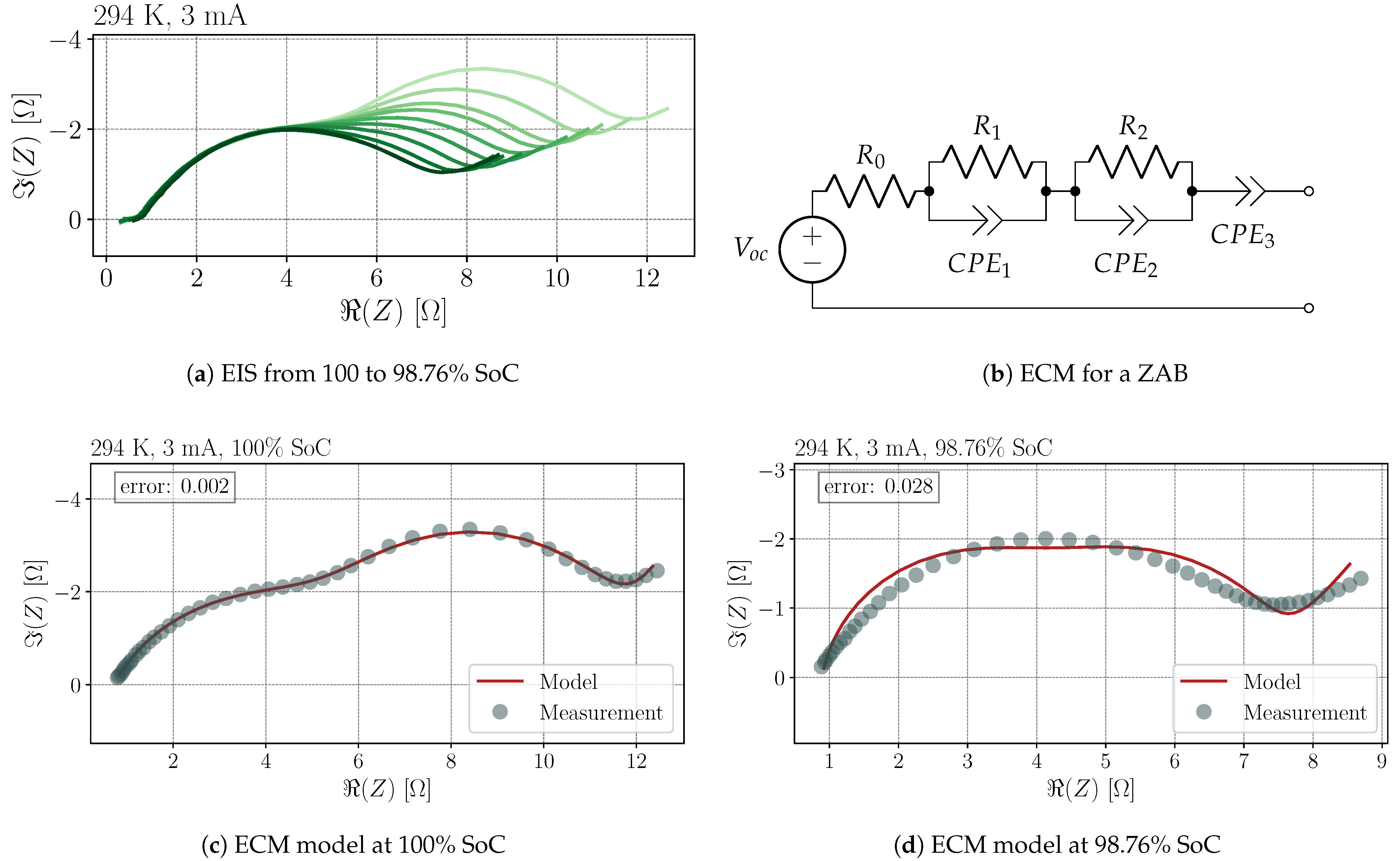
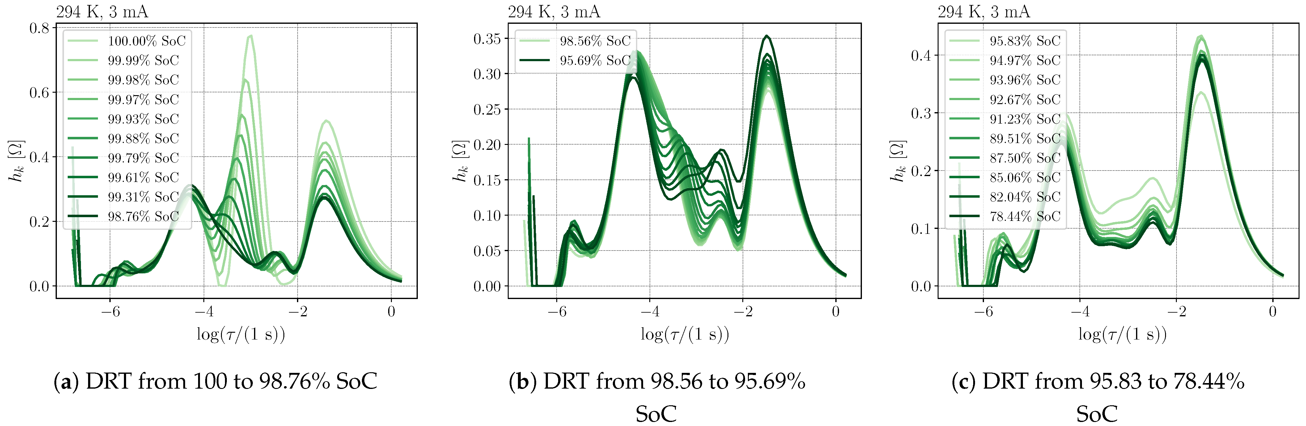
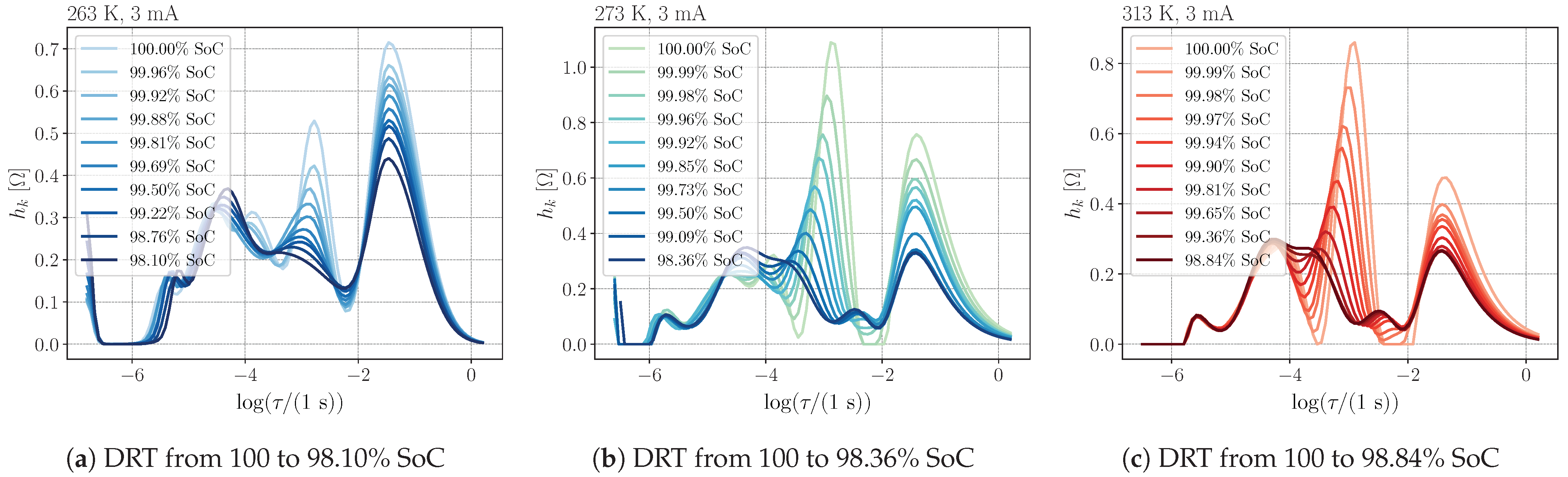
The DRT in Figure 7a and the discharge curves in Figure 6 revealed a very inhomogeneous operating phase, i.e., operating phase I, during the first 10% SoC discharge. The measurement routine, depicted in Figure 1, was not suitable for monitoring this phase because the measurement steps were too large. Therefore, a loop of EIS measurement was performed and the cell was discharged with a superimposed discharge current during the EIS measurement. The corresponding EIS measurements during the first 1% discharge are shown in Figure 8a. Two semicircles and the beginning of the diffusion part were identified for 100% SoC. The second semicircle disappeared for decreasing SoCs. The ECM represents two main processes with each process having a distribution of time constants considered by the constant phase elements (CPE) [66]. Such a construct is a simple method for fitting the impedance data, but without a physical meaning at first [30]. The fit of the ECM related to the EIS measurement at 100% SoC is illustrated in Figure 8c and at 98.76% SoC in Figure 8d. The corresponding values of the ECM are provided in

Table A1. Fitted ECM values from the EIS measurements shown in Figure 8c,d.

SoC	${\mathit{R}}_0$ in $\mathbf{\Omega }$	${\mathit{R}}_1$ in $\mathbf{\Omega }$	${\mathit{R}}_2$ in $\mathbf{\Omega }$	${\mathit{Q}}_1$ in $\mathbf{S}\mathbf{s}\mathbf{n}$	${\mathit{Q}}_2$ in $\mathbf{S}\mathbf{s}\mathbf{n}$	${\mathit{Q}}_3$ in $\mathbf{S}\mathbf{s}\mathbf{n}$	${\mathit{n}}_1$	${\mathit{n}}_2$	${\mathit{n}}_3$
100%	0.80	5.36	5.37	9.4 × ${10}^{-5}$	1.8 × ${10}^{-4}$	1.6 × ${10}^{-2}$	0.77	1.03	0.80
98.76%	0.89	3.22	3.22	2.0 × ${10}^{-5}$	1.8 × ${10}^{-4}$	4.6 × ${10}^{-2}$	0.90	0.88	0.58

. The mean squared error between the simulation and the measurement increased with the disappearance of the second semicircle. The standard fitting procedure could not decide which of the two semicircles disappeared and in which direction the semicircle drifted. The associated DRT in Figure 9a, on the other hand, showed a clear trend. The process at $log\left(\tau \right)\approx -3$ in Figure 9a, which is related to the second semicircle in Figure 8a, was slightly shifted towards $log\left(\tau \right)\approx -4$ and the amplitude was logarithmically decreased during discharge until the process disappeared. While this process was decaying, a new process appeared at $log\left(\tau \right)\approx -2.5$ (see Figure 9c), first steadily increasing to about 5% discharge and then decreasing until a constant value was reached (see Figure 9c). The process at $log\left(\tau \right)\approx -1.5$ decreased in a similar manner to the disappearing process, but stabilized after the first 1% discharge.

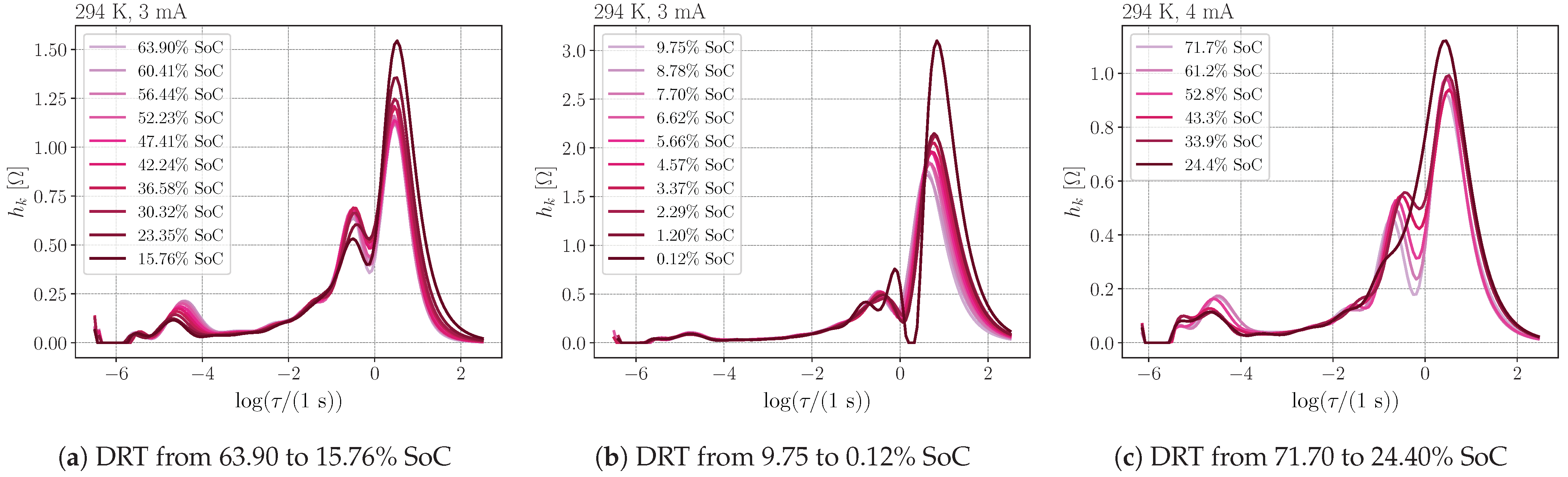
Figure 10 shows that the DRT could also be used for the quantification of operating phase III. Comparing the discharge curves from Figure 6, this phase was not detectable at low currents, which the DRT in Figure 10a reflects. Already, at a discharge current of 4 mA, the process at $log\left(\tau \right)\approx -0.5$ was gradually merging with the process at $log\left(\tau \right)\approx 0.5$ with decreasing SoC. This effect intensified abruptly between 33.9% and 24.4% SoC, as shown in Figure 10c. The end of operating phase IV was also clearly visible in the DRT, evidenced by a sudden increase in resistance at $log\left(\tau \right)\approx 0.5$, illustrated in Figure 10b.

The investigated ZABs showed a temperature dependence (cf. Figure A4); however, operating phase I.1 did not seem to be affected by this dependency. Figure 11 reveals that at all temperatures the process at $log\left(\tau \right)\approx -3$ in operating phase I.1 appeared. The shape of the DRT differed marginally between the temperatures of 273 K and 313 K, but the peaks of the two main processes, i.e., $log\left(\tau \right)\approx -3$ and $log\left(\tau \right)\approx -1.5$, showed a higher resistance towards the lower temperatures, as depicted in Figure 11b,c. With temperatures below 273 K, the process at $log\left(\tau \right)\approx -3$ was tremendously suppressed, showing only half the resistance at 263 K in comparison to 273 K (see Figure 11a).

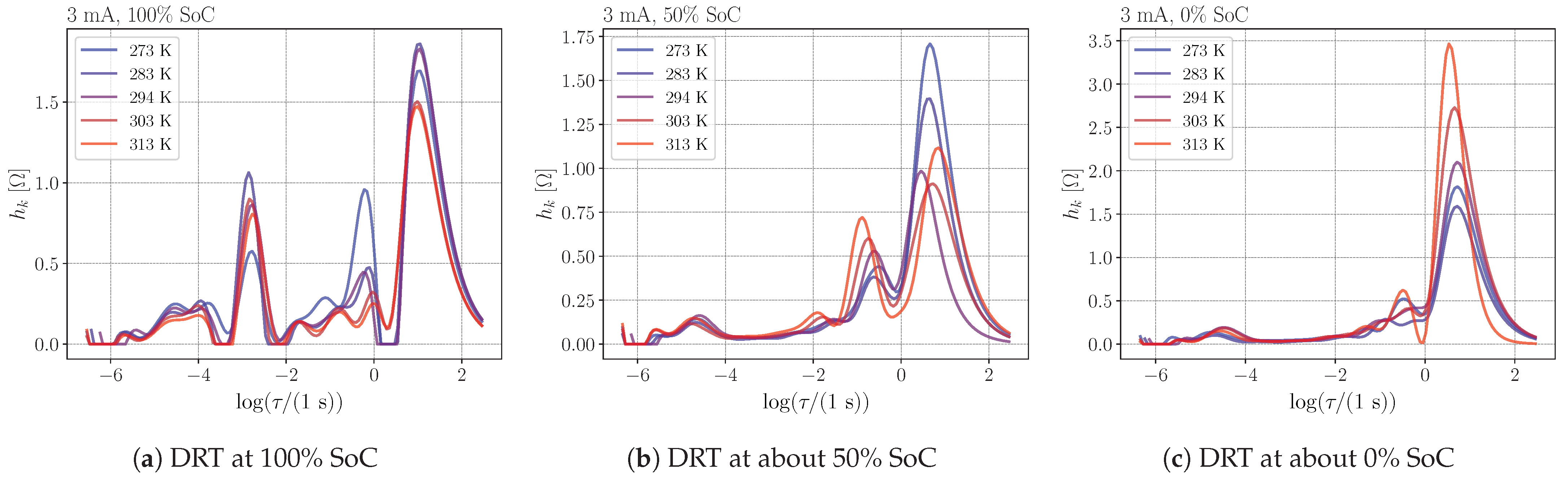
The correlation of the temperature of the DRT at a fixed SoC and a discharge current of 3 mA is shown in Figure 12. The lower the temperatures were, the more significant was the range between $log\left(\tau \right)=-2$ and $log\left(\tau \right)=0$ at an SoC of about 100% (see Figure 12a). It should be critically mentioned here that in contrast to Figure 11, the full frequency range was used for the measurement, which resulted in longer measurement times and a possible inaccuracy. In the medium State-of-Charge related to Figure 12b, this range was more prominent for higher temperatures and, at the same time, the resistance at $log\left(\tau \right)\approx 0.5$ decreased. Finally, for higher temperatures from 294 K, the process at $log\left(\tau \right)\approx 0.5$ became dominant with decreasing SoC (see Figure 12c). The same process, on the other hand, showed no dependence on SoC at 273 K and only a minor dependence at 283 K.

4. Discussion

4.1. Capacity

None of the cells tested could reached the manufacturer’s specification of 300 mAh. This is probably due to the way the capacity was determined. The cells, here, were discharged with a constant discharge current until the cut-off voltage of 0.9 V was reached. In contrast, the standard [67] defines the determination of the operating life via a constant resistance. This in turn leads to a reduced current when the potential drops, so that the load is reduced towards the cut-off voltage and thus more capacity can be obtained. Ingale et al. have shown that the capacity also depends on the ambient humidity and the capacity was halved in dry air compared to 30% relative humidity [68]. Different temperatures in the climatic chamber can lead to different humidities and thus the measurements were probably affected by an unknown error. Penteado and Bento have discussed, beside the deviation of the nominal capacity from the measured capacity of different manufacturers, the average service of the PR48 cell type, which showed a variation of $266\pm 26$ h [69]. These results confirm the capacity measurements in this study that each cell may have a different factory-made capacity. Thus, the determination of the capacity via a separate measurement can only provide valid values for more cells to a limited extent. Therefore, the humidity and the nominal capacity should be critically mentioned in further investigations.

4.2. Operating Phases

First, it is important to understand the basic working principle of a ZAB in order to interpret the data obtained from the DRT. The main process is the oxidation of zinc during discharge. This process does not take place immediately and is characterized by at least one more intermediate step. The electrolyte used is usually 30% potassium hydroxide solution [70], which was also assumed for the cell type studied here. At this concentration, the intermediate step is defined by the formation of zincate Zn(OH)₄2⁻ [71]:

$$\mathrm{Zn}\left(\mathsf{s}\right)+4{\mathrm{OH}}^{-}\left(\mathrm{aq}\right)\mathtt{\rightleftharpoons }\mathrm{Zn}\left(\mathrm{OH}\right)4^{2-}\left(\mathrm{aq}\right)+2{\mathsf{e}}^{-}.$$

(16)

Zinc oxide ZnO precipitates when the critical saturation of zincate in the solution is reached:

$$\mathrm{Zn}\left(\mathrm{OH}\right)4^{2-}\left(\mathrm{aq}\right)\to \mathrm{ZnO}\left(\mathsf{s}\right)+{\mathsf{H}}_2\mathsf{O}\left(\mathsf{l}\right)+2{\mathrm{OH}}^{-}\left(\mathrm{aq}\right).$$

(17)

The consumption of hydroxide ions OH⁻ at the anode is recovered in parallel by the conversion of ambient oxygen O₂ and water H₂O to hydroxide ions at the cathode:

$$\frac{1}{2}{\mathsf{O}}_2(\mathsf{g})+{\mathsf{H}}_2\mathsf{O}(\mathsf{l})+2{\mathsf{e}}^{-}\to 2{\mathrm{OH}}^{-}(\mathrm{aq}).$$

(18)

4.2.1. Operating Phase I

Operating phase I specifies three processes, i.e., I.1, I.2 and I.3, at the initial stage of discharge. Stamm et al. have interpreted process I.2 as a linear increase in zincate concentration and a consumption of hydroxide ions in the anode (see Equation (16)), resulting in a linear voltage drop until the electrolyte was supersaturated [72]. Furthermore, they also have justified Process I.3, which was related to the precipitation of zincate to zinc oxide (see Equation (17)) and thus have increased the hydroxide ions and have reduced the overpotential. Relating these findings to the DRT in Figure 9b, zincate formation I.2 can be applied to the time constant $log({\tau }_{\mathrm{I}}.2)\approx -2.5$ and oxidation of zinc can be applied to the time constant $log({\tau }_{\mathrm{I}}.3)\approx -1.5$. Process I.1 was related to the time constant $log({\tau }_{\mathrm{I}}.1)\approx -3$ and was responsible for the second semicircle within the EIS measurement (cf. Figure 8a). Ma et al. have also observed a second semicircle, which have disappeared with higher superimposed discharge currents or already used cathodes [73]. They have explained the second semicircle with the kinetics of the cathode. The kinetics of a chemical reaction can be described by the reaction rate, which depends, e.g., on the temperature, the concentration or the applied catalysts. Figure 11a demonstrates that although the process I.1 is less dominant at very low temperatures, it decays with similar time steps. Furthermore, the peak is only identifiable at 100% SoC in the DRT even if the cell was relaxed after the discharge steps. Therefore, we hypothesize that the process I.1 describes less the kinetics and more an initial chemical activation of the cathode.

4.2.2. Operating Phase II

In operating phase II, an equilibrium of the presented reactions (16)–(18) has already been reached. A constant deposition of zinc oxide follows, as long as no passivation occurs within the porous anode [15] or secondary processes occur in the cathode, e.g., flooding [74] or pore clogging [75]. The DRT in Figure 7 shows no significant variation between 20 and 70% discharge capacity and currents up to a maximum of 4 mA, which is a characteristic of stable and constant reactions. Since the process with time constant $log\left(\tau \right)\approx 1$ can be assigned to diffusion [37], the peak $log\left(\tau \right)\approx -1$ is distinctive for oxidation of zinc and the peak $log\left(\tau \right)\approx -4.5$ represents the recovery of hydroxide ions at the cathode.

4.2.3. Operating Phase III and IV

Operating phase III represents the voltage step during discharge that was detectable for currents above 3 mA. Two theories have been proposed for this behavior. The first has discussed two different oxidation states of zinc, i.e., “solid-state” and “dissolution-precipitation” [15]. In this case, the “solid-state” oxidation was observable only at higher overpotentials, which could be caused by higher discharge currents or by depletion of hydroxide ions in the anode. The second study has attributed the voltage step to the inhomogeneous nucleation of the zinc oxide [72]. Specifically, the simulation has shown that the zincate has precipitated near the current collector rather than at the separator and thus has coated the unused zinc with an oxide layer. Overcoming the oxide layer in the later discharge process, was the reason for the voltage drop. The latter study does not coincide with tomography images of the discharge process of ZABs, where a significant oxidation of the zinc accompanied by a shape change have begun near the separator [76,77]. Therefore, we assume that the voltage step is caused by a hindered mass transport due to shape change and volume expansion. Figure 10c shows that with higher currents or at the end of the discharge (cf. Figure 10b), the oxidation process merged into the diffusion process. The operating phase IV is finally the termination of the zinc oxidation (see Figure 10b), which is caused by the complete consumption of zinc or by the formation of a diffusion barrier.

4.3. Temperature

Decreasing the ambient temperature has a similar effect on the discharge capacity as increasing the current. The lower the temperature, the higher the ohmic overpotential and the lower the capacity (cf. Figure 6 and Figure A4). The ambient temperature in general has a complex influence on the entire system, i.e., on all transport processes, on reaction kinetics, on reaction potentials and overpotentials and on the material properties [78]. The electrolyte contributes most to the decreasing potential as the temperature decreases [70], e.g., conductivity decreases approximately linearly with decreasing temperatures [79]. According to the Einstein relation, diffusion is hindered to the same extent, which can lead to limited utilization of the zinc anode at a constant current. The DRT in Figure 12 reveals that the oxidation of zinc was suppressed by lower temperatures and that the diffusion process was nearly constant. Figure 11 also shows that activation of the cathode was tremendously inhibited by temperatures below 273 K.

4.4. Shortcomings

Figure 8a shows an ECM that is sometimes used for modeling of ZABs or sub-processes [26,80,81,82]. This ECM provides good results here for 100% SoC (see Figure 8c). However, with the disappearance of the second semicircle after 1% discharge, the model is overparameterized and thus, without any further adaption, unsuitable (see Figure 8d). The DRT, on the other hand, provides an approach that bypasses an accurate knowledge of a suitable model. With appropriate post-processing functions, individual parameters can also be quantified as shown in Table 2. For a correct quantification, however, some parameters of the DRT have to be considered critically:

• The regularization parameter directly influences the number and heights of the peaks within the DRT (see Figure A3). Each EIS measurement may have its own optimal regularization parameter, so that an estimation of the parameter must be made over all data (cf. Figure 5). It is not guaranteed that there will be an ideal parameter for the entire data set.
• The intersection of the EIS measurement with the real axis is not always given at high frequencies and no $\Im \left\{Z_{\mathrm{Meas}}\right\}=0$ exists. The intersection point for the DRT must consequently be estimated for the initial condition, which leads to an additional peak and a minimization of the other peaks according to Equation (12). This shortcoming can be avoided by pre-processing the EIS measurement.
• The extended time constant range and the extended boundary at low frequencies improve the physical interpretation of the DRT but manipulate the height of the peaks.

5. Conclusions

The applicability of the DRT to the process analysis of ZABs was confirmed for the first time. The findings and the simulations from the literature could be covered by the DRT, which opens up new possibilities in the simulation and analysis of ZABs. For example, the cathode activation process and also the current dependence of the oxidation of zinc could be identified by this technique. The method presented here for the determination of the regularization parameter is based on the comparison of the reconstructed data from a Gaussian probability distribution function and the impedance values from the EIS measurement. This method can provide a good estimate of a suitable regularization parameter, but should always be verified in terms of plausibility with the available measurements. Since the capacity spread of the primary cells were wide, which made it difficult to approach the targeted SoC values, future studies should use only a repeating EIS with superimposed current and should calculate the capacity retrospectively.

References

- Li, M.; Lu, J.; Chen, Z.; Amine, K. 30 Years of Lithium-Ion Batteries. Adv. Mater. 2018, 30, 1800561. [Google Scholar] [CrossRef] [Green Version]
- Caramia, V.; Bozzini, B. Materials science aspects of zinc-air batteries: A review. Mater. Renew. Sustain. Energy 2014, 3, 28. [Google Scholar] [CrossRef] [Green Version]
- Yi, J.; Liang, P.; Liu, X.; Wu, K.; Liu, Y.; Wang, Y.; Xia, Y.; Zhang, J. Challenges, mitigation strategies and perspectives in development of zinc-electrode materials and fabrication for rechargeable zinc–air batteries. Energy Environ. Sci. 2018, 11, 3075–3095. [Google Scholar] [CrossRef] [Green Version]
- Pan, J.; Xu, Y.Y.; Yang, H.; Dong, Z.; Liu, H.; Xia, B.Y. Advanced Architectures and Relatives of Air Electrodes in Zn–Air Batteries. Adv. Sci. 2018, 5, 1700691. [Google Scholar] [CrossRef]
- Zhang, J.; Zhou, Q.; Tang, Y.; Zhang, L.; Li, Y. Zinc-air batteries: Are they ready for prime time? Chem. Sci. 2019, 10, 8924–8929. [Google Scholar] [CrossRef] [PubMed] [Green Version]
- Fu, J.; Cano, Z.P.; Park, M.G.; Yu, A.; Fowler, M.; Chen, Z. Electrically Rechargeable Zinc–Air Batteries: Progress, Challenges, and Perspectives. Adv. Mater. 2017, 29, 1604685. [Google Scholar] [CrossRef] [PubMed]
- Pei, P.; Wang, K.; Ma, Z. Technologies for extending zinc-air battery’s cyclelife: A review. Appl. Energy 2014, 128, 315–324. [Google Scholar] [CrossRef]
- Gu, P.; Zheng, M.; Zhao, Q.; Xiao, X.; Xue, H.; Pang, H. Rechargeable zinc-air batteries: A promising way to green energy. J. Mater. Chem. A 2017, 5, 7651–7666. [Google Scholar] [CrossRef]
- Shin, J.; Lee, J.; Park, Y.; Choi, J.W. Aqueous zinc ion batteries: Focus on zinc metal anodes. Chem. Sci. 2020, 11, 2028–2044. [Google Scholar] [CrossRef] [Green Version]
- Stock, D.; Dongmo, S.; Damtew, D.; Stumpp, M.; Konovalova, A.; Henkensmeier, D.; Schlettwein, D.; Schröder, D. Design Strategy for Zinc Anodes with Enhanced Utilization and Retention: Electrodeposited Zinc Oxide on Carbon Mesh Protected by Ionomeric Layers. ACS Appl. Energy Mater. 2018, 1, 5579–5588. [Google Scholar] [CrossRef]
- Riede, J.C.; Turek, T.; Kunz, U. Critical zinc ion concentration on the electrode surface determines dendritic zinc growth during charging a zinc air battery. Electrochim. Acta 2018, 269, 217–224. [Google Scholar] [CrossRef]
- Mainar, A.R.; Colmenares, L.C.; Grande, H.J.J.; Blázquez, J.A. Enhancing the cycle life of a Zinc–air battery by means of electrolyte additives and zinc surface protection. Batteries 2018, 4, 46. [Google Scholar] [CrossRef] [Green Version]
- Mainar, A.R.; Colmenares, L.C.; Blázquez, J.A.; Urdampilleta, I. A brief overview of secondary zinc anode development: The key of improving zinc-based energy storage systems. Int. J. Energy Res. 2018, 42, 903–918. [Google Scholar] [CrossRef]
- Stock, D.; Dongmo, S.; Walther, F.; Sann, J.; Janek, J.; Schröder, D. Homogeneous Coating with an Anion-Exchange Ionomer Improves the Cycling Stability of Secondary Batteries with Zinc Anodes. ACS Appl. Mater. Interfaces 2018, 10, 8640–8648. [Google Scholar] [CrossRef]
- Bockelmann, M.; Becker, M.; Reining, L.; Kunz, U.; Turek, T. Passivation of Zinc Anodes in Alkaline Electrolyte: Part I. Determination of the Starting Point of Passive Film Formation. J. Electrochem. Soc. 2018, 165, A3048–A3055. [Google Scholar] [CrossRef]
- Bockelmann, M.; Becker, M.; Reining, L.; Kunz, U.; Turek, T. Passivation of Zinc Anodes in Alkaline Electrolyte: Part II. Influence of Operation Parameters. J. Electrochem. Soc. 2019, 166, A1132–A1139. [Google Scholar] [CrossRef]
- Cai, M.; Park, S.M. Spectroelectrochemical Studies on Dissolution and Passivation of Zinc Electrodes in Alkaline Solutions. J. Electrochem. Soc. 1996, 143, 2125. [Google Scholar] [CrossRef]
- Kim, H.I.; Kim, E.J.; Kim, S.J.; Shin, H.C. Influence of ZnO precipitation on the cycling stability of rechargeable Zn–air batteries. J. Appl. Electrochem. 2015, 45, 335–342. [Google Scholar] [CrossRef]
- Franke-Lang, R.; Arlt, T.; Manke, I.; Kowal, J. X-ray tomography as a powerful method for zinc-air battery research. J. Power Sources 2017, 370, 45–51. [Google Scholar] [CrossRef]
- Wang, H.F.; Xu, Q. Materials Design for Rechargeable Metal-Air Batteries. Matter 2019, 1, 565–595. [Google Scholar] [CrossRef]
- Macdonald, J.R. Impedance spectroscopy. Ann. Biomed. Eng. 1992, 20, 289–305. [Google Scholar] [CrossRef] [PubMed]
- Fu, J.; Zhang, J.; Song, X.; Zarrin, H.; Tian, X.; Qiao, J.; Rasen, L.; Li, K.; Chen, Z. A flexible solid-state electrolyte for wide-scale integration of rechargeable zinc-air batteries. Energy Environ. Sci. 2016, 9, 663–670. [Google Scholar] [CrossRef]
- Sanal, E.; Dost, P.; Sourkounis, C. Electrotechnical investigation of zinc-air cells for determination of cell-parameters for a battery management system. In Proceedings of the 2015 International Conference on Renewable Energy Research and Applications (ICRERA), Palermo, Italy, 22–25 November 2015; pp. 1157–1161. [Google Scholar] [CrossRef]
- Larsson, F.; Rytinki, A.; Ahmed, I.; Albinsson, I.; Mellander, B.E. Overcurrent abuse of primary prismatic zinc–air battery cells studying air supply effects on performance and safety shut-down. Batteries 2017, 3, 1. [Google Scholar] [CrossRef] [Green Version]
- Meng, F.; Zhong, H.; Bao, D.; Yan, J.; Zhang, X. In Situ Coupling of Strung Co 4 N and Intertwined N–C Fibers toward Free-Standing Bifunctional Cathode for Robust, Efficient, and Flexible Zn–Air Batteries. J. Am. Chem. Soc. 2016, 138, 10226–10231. [Google Scholar] [CrossRef] [PubMed]
- Li, G.; Zhang, K.; Mezaal, M.A.; Zhang, R.; Lei, L. Effect of electrolyte concentration and depth of discharge for zinc-air fuel cell. Int. J. Electrochem. Sci. 2015, 10, 6672–6683. [Google Scholar]
- Chotipanich, J.; Arpornwichanop, A.; Yonezawa, T.; Kheawhom, S. Electronic and ionic conductivities enhancement of zinc anode for flexible printed zinc-air battery. Eng. J. 2018, 22, 47–57. [Google Scholar] [CrossRef]
- Kubannek, F.; Turek, T.; Krewer, U. Modeling Oxygen Gas Diffusion Electrodes for Various Technical Applications. Chemie-Ingenieur-Technik 2019, 91, 720–733. [Google Scholar] [CrossRef] [Green Version]
- Tran, T.N.T.; Chung, H.J.; Ivey, D.G. A study of alkaline gel polymer electrolytes for rechargeable zinc–air batteries. Electrochim. Acta 2019, 327, 135021. [Google Scholar] [CrossRef]
- Barsoukov, E.; Macdonald, J.R. (Eds.) Impedance Spectroscopy, 3rd ed.; John Wiley & Sons, Inc.: Hoboken, NJ, USA, 2018; pp. 1–528. [Google Scholar] [CrossRef]
- Vielstich, W.; Hamann, C.H. Elektrochemie; Wiley-VCH: Weinheim, Germany, 2005; p. 662. [Google Scholar] [CrossRef]
- Weiß, A.; Schindler, S.; Galbiati, S.; Danzer, M.A.; Zeis, R. Distribution of Relaxation Times Analysis of High-Temperature PEM Fuel Cell Impedance Spectra. Electrochim. Acta 2017, 230, 391–398. [Google Scholar] [CrossRef]
- Ivers-Tiffée, E.; Weber, A. Evaluation of electrochemical impedance spectra by the distribution of relaxation times. J. Ceram. Soc. Jpn. 2017, 125, 193–201. [Google Scholar] [CrossRef] [Green Version]
- Schichlein, H.; Müller, A.C.; Voigts, M.; Krügel, A.; Ivers-Tiffée, E. Deconvolution of electrochemical impedance spectra for the identification of electrode reaction mechanisms in solid oxide fuel cells. J. Appl. Electrochem. 2002, 32, 875–882. [Google Scholar] [CrossRef]
- Hahn, M.; Schindler, S.; Triebs, L.C.; Danzer, M.A. Optimized process parameters for a reproducible distribution of relaxation times analysis of electrochemical systems. Batteries 2019, 5, 43. [Google Scholar] [CrossRef] [Green Version]
- Hahn, M.; Rosenbach, D.; Krimalowski, A.; Nazarenus, T.; Moos, R.; Thelakkat, M.; Danzer, M.A. Investigating solid polymer and ceramic electrolytes for lithium-ion batteries by means of an extended Distribution of Relaxation Times analysis. Electrochim. Acta 2020, 344, 136060. [Google Scholar] [CrossRef]
- Danzer, M.A. Generalized distribution of relaxation times analysis for the characterization of impedance spectra. Batteries 2019, 5, 53. [Google Scholar] [CrossRef] [Green Version]
- Ciucci, F.; Chen, C. Analysis of electrochemical impedance spectroscopy data using the distribution of relaxation times: A Bayesian and hierarchical Bayesian approach. Electrochim. Acta 2015, 167, 439–454. [Google Scholar] [CrossRef]
- Schlüter, N.; Ernst, S.; Schröder, U. Direct Access to the Optimal Regularization Parameter in Distribution of Relaxation Times Analysis. ChemElectroChem 2020, 7, 3445–3458. [Google Scholar] [CrossRef]
- Boukamp, B.A. Fourier transform distribution function of relaxation times; application and limitations. Electrochim. Acta 2015, 154, 35–46. [Google Scholar] [CrossRef]
- Boukamp, B.A.; Rolle, A. Analysis and Application of Distribution of Relaxation Times in Solid State Ionics. Solid State Ion. 2017, 302, 12–18. [Google Scholar] [CrossRef]
- Effat, M.B.; Ciucci, F. Bayesian and Hierarchical Bayesian Based Regularization for Deconvolving the Distribution of Relaxation Times from Electrochemical Impedance Spectroscopy Data. Electrochim. Acta 2017, 247, 1117–1129. [Google Scholar] [CrossRef]
- Hörlin, T. Deconvolution and maximum entropy in impedance spectroscopy of noninductive systems. Solid State Ion. 1998, 107, 241–253. [Google Scholar] [CrossRef]
- Liu, J.; Ciucci, F. The Gaussian process distribution of relaxation times: A machine learning tool for the analysis and prediction of electrochemical impedance spectroscopy data. Electrochim. Acta 2020, 331, 135316. [Google Scholar] [CrossRef]
- Liu, J.; Ciucci, F. The Deep-Prior Distribution of Relaxation Times. J. Electrochem. Soc. 2020, 167, 026506. [Google Scholar] [CrossRef]
- Tuncer, E.; Gubanski, S. On dielectric data analysis. Using the Monte Carlo method to obtain relaxation time distribution and comparing non-linear spectral function fits. IEEE Trans. Dielectr. Electr. Insul. 2001, 8, 310–320. [Google Scholar] [CrossRef]
- Ross Macdonald, J. Comparison of parametric and nonparametric methods for the analysis and inversion of immittance data: Critique of earlier work. J. Comput. Phys. 2000, 157, 280–301. [Google Scholar] [CrossRef]
- Bello, A.; Laredo, E.; Grimau, M. Distribution of relaxation times from dielectric spectroscopy using Monte Carlo simulated annealing: α-PVDF. Phys. Rev. B 1999, 60, 12764–12774. [Google Scholar] [CrossRef]
- Tesler, A.B.; Lewin, D.R.; Baltianski, S.; Tsur, Y. Analyzing results of impedance spectroscopy using novel evolutionary programming techniques. J. Electroceram. 2010, 24, 245–260. [Google Scholar] [CrossRef]
- Hershkovitz, S.; Baltianski, S.; Tsur, Y. Harnessing evolutionary programming for impedance spectroscopy analysis: A case study of mixed ionic-electronic conductors. Solid State Ion. 2011, 188, 104–109. [Google Scholar] [CrossRef]
- Saccoccio, M.; Wan, T.H.; Chen, C.; Ciucci, F. Optimal regularization in distribution of relaxation times applied to electrochemical impedance spectroscopy: Ridge and Lasso regression methods—A theoretical and experimental Study. Electrochim. Acta 2014, 147, 470–482. [Google Scholar] [CrossRef]
- Wan, T.H.; Saccoccio, M.; Chen, C.; Ciucci, F. Influence of the Discretization Methods on the Distribution of Relaxation Times Deconvolution: Implementing Radial Basis Functions with DRTtools. Electrochim. Acta 2015, 184, 483–499. [Google Scholar] [CrossRef]
- Žic, M.; Pereverzyev, S.; Subotić, V.; Pereverzyev, S. Adaptive multi-parameter regularization approach to construct the distribution function of relaxation times. GEM Int. J. Geomath. 2020, 11, 1–23. [Google Scholar] [CrossRef] [PubMed] [Green Version]
- Gavrilyuk, A.L.; Osinkin, D.A.; Bronin, D.I. The use of Tikhonov regularization method for calculating the distribution function of relaxation times in impedance spectroscopy. Russ. J. Electrochem. 2017, 53, 575–588. [Google Scholar] [CrossRef]
- Schlüter, N.; Ernst, S.; Schröder, U. Finding the Optimal Regularization Parameter in Distribution of Relaxation Times Analysis. ChemElectroChem 2019, 6, 6027–6037. [Google Scholar] [CrossRef] [Green Version]
- Li, X.; Ahmadi, M.; Collins, L.; Kalinin, S.V. Deconvolving distribution of relaxation times, resistances and inductance from electrochemical impedance spectroscopy via statistical model selection: Exploiting structural-sparsity regularization and data-driven parameter tuning. Electrochim. Acta 2019, 313, 570–583. [Google Scholar] [CrossRef]
- Nickol, A.; Schied, T.; Heubner, C.; Schneider, M.; Michaelis, A.; Bobeth, M.; Cuniberti, G. GITT Analysis of Lithium Insertion Cathodes for Determining the Lithium Diffusion Coefficient at Low Temperature: Challenges and Pitfalls. J. Electrochem. Soc. 2020, 167, 090546. [Google Scholar] [CrossRef]
- Lawson, C.L.; Hanson, R.J. Solving Least Squares Problems; Society for Industrial and Applied Mathematics: Philadelphia, PA, USA, 1995; p. 337. [Google Scholar] [CrossRef]
- Marquardt, D.W. An Algorithm for Least-Squares Estimation of Nonlinear Parameters. J. Soc. Ind. Appl. Math. 1963, 11, 431–441. [Google Scholar] [CrossRef]
- Kraft, D. A Software Package for Sequential Quadratic Programming; Wiss. Berichtswesen d. DFVLR: Köln, Germany, 1988. [Google Scholar]
- Byrd, R.H.; Lu, P.; Nocedal, J.; Zhu, C. A Limited Memory Algorithm for Bound Constrained Optimization. SIAM J. Sci. Comput. 1995, 16, 1190–1208. [Google Scholar] [CrossRef]
- Tikhonov, A.N.; Goncharsky, A.V.; Stepanov, V.V.; Yagola, A.G. Numerical Methods for the Solution of Ill-Posed Problems; Springer: Dordrecht, The Netherlands, 1995. [Google Scholar] [CrossRef]
- Hansen, J.K.; Hogue, J.D.; Sander, G.K.; Renaut, R.A.; Popat, S.C. Non-negatively constrained least squares and parameter choice by the residual periodogram for the inversion of electrochemical impedance spectroscopy data. J. Comput. Appl. Math. 2015, 278, 52–74. [Google Scholar] [CrossRef]
- Korth Pereira Ferraz, P.; Kowal, J. A Comparative Study on the Influence of DC/DC-Converter Induced High Frequency Current Ripple on Lithium-Ion Batteries. Sustainability 2019, 11, 6050. [Google Scholar] [CrossRef] [Green Version]
- Agarwal, P.; Orazem, M. Measurement Models for Electrochemical Impedance Spectroscopy. J. Electrochem. Soc. 1992, 139, 1917. [Google Scholar] [CrossRef]
- Orazem, M.E.; Tribollet, B. Electrochemical Impedance Spectroscopy; John Wiley & Sons, Inc.: Hoboken, NJ, USA, 2017; pp. 1–523. [Google Scholar] [CrossRef]
- Deutsches Institut für Normung e.V. International Standard: Primary Batteries—Part 2: Physical and Electrical Specifications (IEC 60086-2:2015); Beuth-Verlag: Berlin, Germany, 2016. [Google Scholar] [CrossRef]
- Ingale, P.; Sakthivel, M.; Drillet, J.F. Test of Diethylmethylammonium Trifluoromethanesulfonate Ionic Liquid as Electrolyte in Electrically Rechargeable Zn/Air Battery. J. Electrochem. Soc. 2017, 164, H5224–H5229. [Google Scholar] [CrossRef]
- Penteado, S.P.; Bento, R.F. Performance analysis of ten brands of batteries for hearing aids. Int. Arch. Otorhinolaryngol. 2013, 17, 291–304. [Google Scholar] [CrossRef] [Green Version]
- Reddy, T.B. Linden’s Handbook of Batteries, 4th ed.; McGraw-Hill Education: New York, NY, USA, 2011. [Google Scholar]
- Clark, S.; Mainar, A.R.; Iruin, E.; Colmenares, L.C.; Blázquez, J.A.; Tolchard, J.R.; Jusys, Z.; Horstmann, B. Designing Aqueous Organic Electrolytes for Zinc–Air Batteries: Method, Simulation, and Validation. Adv. Energy Mater. 2020, 10. [Google Scholar] [CrossRef]
- Stamm, J.; Varzi, A.; Latz, A.; Horstmann, B. Modeling nucleation and growth of zinc oxide during discharge of primary zinc-air batteries. J. Power Sources 2017, 360, 136–149. [Google Scholar] [CrossRef] [Green Version]
- Ma, Z.; Pei, P.; Wang, K.; Wang, X.; Xu, H.; Liu, Y.; Peng, G. Degradation characteristics of air cathode in zinc air fuel cells. J. Power Sources 2015, 274, 56–64. [Google Scholar] [CrossRef]
- Schröder, D.; Arlt, T.; Krewer, U.; Manke, I. Analyzing transport paths in the air electrode of a zinc air battery using X-ray tomography. Electrochem. Commun. 2014, 40, 88–91. [Google Scholar] [CrossRef]
- Tsehaye, M.T.; Alloin, F.; Iojoiu, C.; Tufa, R.A.; Aili, D.; Fischer, P.; Velizarov, S. Membranes for zinc-air batteries: Recent progress, challenges and perspectives. J. Power Sources 2020, 475, 228689. [Google Scholar] [CrossRef]
- Schmitt, T.; Arlt, T.; Manke, I.; Latz, A.; Horstmann, B. Zinc electrode shape-change in secondary air batteries: A 2D modeling approach. J. Power Sources 2019, 432, 119–132. [Google Scholar] [CrossRef] [Green Version]
- Arlt, T.; Schröder, D.; Krewer, U.; Manke, I. In operando monitoring of the state of charge and species distribution in zinc air batteries using X-ray tomography and model-based simulations. Phys. Chem. Chem. Phys. 2014, 16, 22273–22280. [Google Scholar] [CrossRef] [PubMed] [Green Version]
- Franke-lang, R.; Kowal, J. Electrochemical Model-Based Investigation of Thick LiFePO4 Electrode Design Parameters. Modelling 2021, 2, 259–287. [Google Scholar] [CrossRef]
- See, D.M.; White, R.E. Temperature and concentration dependence of the specific conductivity of concentrated solutions of potassium hydroxide. J. Chem. Eng. Data 1997, 42, 1266–1268. [Google Scholar] [CrossRef]
- Zhuang, S.; Zhang, H.; Liu, S.; Tu, F.; Zhang, W.; Zhao, C. Optimized perovskite electrocatalyst for bifunctional air electrode by impedance spectroscopy analysis. Int. J. Electrochem. Sci. 2014, 9, 1690–1701. [Google Scholar]
- Hoang, T.K.A.; Doan, T.N.L.; Sun, K.E.K.; Chen, P. Corrosion chemistry and protection of zinc & zinc alloys by polymer-containing materials for potential use in rechargeable aqueous batteries. RSC Adv. 2015, 5, 41677–41691. [Google Scholar] [CrossRef]
- Thomas Goh, F.W.; Liu, Z.; Hor, T.S.A.; Zhang, J.; Ge, X.; Zong, Y.; Yu, A.; Khoo, W. A Near-Neutral Chloride Electrolyte for Electrically Rechargeable Zinc-Air Batteries. J. Electrochem. Soc. 2014, 161, A2080–A2086. [Google Scholar] [CrossRef]
Figure 1.
Discharge curve of a ZAB (b) at 303 K with a constant current of 3 mA. The red circles indicate the point where the EIS measurement was taken. (a) Illustrates the inhomogeneous discharge behavior separated in three different sub-processes during the discharge of the first 10% SoC.
Figure 2.
EIS measurement of a ZAB at 298 K and SoC of 100%. The red marked area shows the transition to the inductive parts which is not considered by default (1), (2) is the area that can be described well via the DRT, and (3) represents a sensitive area.
Figure 3.
Problem of a not converging EIS measurement at low frequencies. The main peak in the DRT (b) is attributable to the diffusion part, which leads to higher regularization parameters and thus larger deviations (a) in the reconstruction.
Figure 4.
Comparison of different minimization algorithms: Powell, TNC, SLSQP, and L-BFGS-B. The SLSQP algorithm shows the same result as the NNLS algorithm. The regularization parameter influences the DRT (see Equation (12)) with increasing values and smooths the peaks.
Figure 5.
Calculation of the regularization parameter depending on the temperatures between 273 K and 313 K as well as on the currents 3 mA to 6 mA. A boxplot represents the calculation of at each measured SoC. The black line within the box indicates the median and the circles show outliers.
Figure 6.
ZAB PR48 discharge profiles at 294 K and various constant discharge currents from 2 mA to 10 mA. The annotations I–IV represent different operating phases of the cell.
Figure 7.
Process analysis of a ZAB at 303 K via the DRT related to different currents and SoCs.
Figure 8.
Process analysis of a ZAB at 294 K and a discharge current of 3 mA. (a) shows the EIS and (b) represents a corresponding equivalent circuit. (c,d) depict the reconstructed EIS from the ECM.
Figure 9.
Process analysis of the first and second operating phase of a ZAB at 294 K and a discharge current of 3 mA. (a,c) represent 10 logarithmically extracted values from the data set, respectively, and (b) depicts 20 linear SOC steps in a range from 98.56% to 95.69% SoC.
Figure 10.
Process analysis of a ZAB at 294 K with (a,b) at 3mA and (c) with 4 mA discharge current.
Figure 11.
Analysis of operating phase I at different temperatures at 3 mA discharge current.
Figure 12.
Influence of temperature at different SoCs and a discharge current of 3 mA.