1. Introduction
Everyday, space-borne and airborne sensors deliver a huge number of Earth observation data so that we can observe the whole Earth from different angles. Therefore, this data is the main actor for big data in remote sensing and it can be used in several domains such as monitoring, climate change, agriculture, and urban planning. Indeed, to introduce Big data is to determine its Vs: volume, velocity, variety and veracity. These four Vs [
1] are the most widespread and they can go up to 13 Vs and more [
2]. Images delivered by different sensors, whether active or passive, have become more and more accessible. This type of data is used in several fields and that is why we are introducing the term Big Remote Sensing Data (BRSD), this denomination linking the two domains: big data and remote sensing. What we have to know is how these Vs are used in BRSD.
Obviously, the complexity of massive satellite data stems from the variety of different resolution like spatial, spectral and even temporal, which resides in metadata organized into complex structured data. In addition, the distribution of massive satellite data makes their management and exploitation almost complex.
Since the appearance of big data, several tools and frameworks have appeared to analyze a large amount of data such as Hadoop [
3], MapReduce [
4], Spark [
5] and many others. We are interested to work on remote sensing images, a complex type of data, for that, we have to use an efficient big data pipeline [
6] shown in the following
Figure 1.
Looking at the large volume collected every day from the earth observation scene, the first thoughts are how to store them [
7], how many storage layers we need, how long do we need to store the data and can we archive or delete data. Storage refers to systems where data is stored and preserved in completely different steps because it moves through the pipeline. Data storage decisions rely on numerous factors, for instance, the quantity of information, frequency, the number of queries to a storage system, and uses of data for the ensuing step.
Data processing depends on the storing model of the satellite image and refers to image processing. The Hadoop framework is introduced that depends on the MapReduce programming model and the Hadoop distributed file system [
8], which can prepare, store, and analyze a lot of circulated unstructured information.
Apache Spark works on top of the current HDFS system to provide improved and additional services. It brings MapReduce to the next stage with less costly data shuffles with capabilities such as in-memory data storage and real-time processing. Consequently, the outputs are often many times quicker than other big data technologies.
With the appearance of deep learning (DL) in recent years, satellite image analysis approaches have enabled significant advances. It has opened up new possibilities for the research and development of new methods and approaches for satellite image analysis. Therefore, the DL has become the essential solution for solving remote sensing problems like classification and clustering [
9].
In the era of massive data, deep learning shows very interesting perspectives. It is experiencing unprecedented success in many applications. DL uses machine learning techniques involving supervised and/or unsupervised strategies to learn hierarchical representations in deep architectures. DL uses deep architectures in order to deal with complex relationships between the input data and the class label. DL and ensemble-based algorithms were very popular and efficient for multisource and multitemporal remote sensing image classification. They perform better than SVM (Support Vector Machine) as the DL can deal not only with optical images but also with radar images. DL showed a better performance in extracting features from hyperspectral and multispectral images such as extracting types of labels [
10], pixel-based classification, semantic segmentation, and recognition of objects and classes.
Deep learning algorithms learn features from the data; low-level features are extracted from the texture and spectral and they are considered as the bottom level while the top level is the representation of the output features.
In fact, many approaches [
11] have shown that the performance of land cover scene classification has considerably improved as a result of the powerful feature to the powerful feature representation learned through different deep learning architectures.
The most famous two frameworks that we can use in deep learning for our case are Apache Spark [
5] and TensorFlow [
12]. TensorFlow (TF) is an open-source framework destined for machine learning. Tensorflow has built-in support for DL and Neural Network (NN), it is simple to put together a network, assign parameters, and run the training process. Tensorflow also includes a library of simple, trainable mathematic functions useful for NN.
TF is compatible with many variants of machine learning algorithms due to its large collection of flexible tools. Besides, TensorFlow uses CPUs (Central Processing Unit) and GPUs (Graphics Processing Unit) for computing and that quickens the compile-time [
13].
Apache Spark [
14] is another open-source parallel computing framework that benefits from Mapreduce. It provides the flexibility, scalability, and speed required to meet the challenges of big data. Spark incorporates two major libraries: SQL (Structured Query Language) for querying large amounts of structured data, as well as MLlib [
15], which contains the main learning algorithms and statistical methods.
The remainder of this paper is structured as follows. The related work is presented in
Section 2. The proposed approach is described in
Section 3.
Section 4 describes our experimentation and results.
Section 5 contains a brief conclusion with recommendations for future research.
2. Related Works
We have explored what big remote sensing data are, thus their importance and complex properties. The demand for storing and processing big datasets has encouraged the development of data storage and database systems in recent years as well as various platforms for processing and analyzing these data. With this advancement, the analysis systems and data models for big data have been improved over time. Storage methods and techniques have undergone an unprecedented transformation that favors the distribution of data through the use of clusters and clouds.
We will present various applications of CNN architecture that are among the most recent for the treatment of satellite images; specifically, those that are related to satellite image classification and segmentation. We will also discuss the various implementation variations of this type of architecture. DL is gaining popularity in remote sensing, and many papers on various applications of deep learning in remote sensing have been published [
16]. When compared to other methods, deep feature learning architecture can learn semantic features and achieve better classification [
17].
Kussul et al. [
18] proposed a multilevel deep learning architecture and used multitemporal images that the Sentinel-1A and Landsat-8 satellites collected. The proposed architecture consists of four levels; it includes Preprocessing (level1), supervised classification (level2), postprocessing (level3) and final geospatial analysis (level4). 1-D and 2D models To investigate spectral and spatial features, CNN architectures are proposed. Self-organizing Kohenen maps (SOMs) are chosen for optical image segmentation and missing data restoration at the preprocessing level. SOMs are trained separately for each spectral band.
The missing values in the data are restored using a procedure that replaces the missing components in the input samples with the neurons’ weight coefficient. The pixels that have been restored are masked. The second level (Supervised Classification with CNN) compares two different CNN architectures: 1D CNN with convolutions in the spectral domain and 2D CNN with convolutions in the spatial domain. The second level (supervised classification with CNN) compares two different CNN architectures: Convolutions in the spectral domain are used in 1D CNN, while convolutions in the spatial domain are used in 2D CNN.
Both architectures are made up of two convolution layers, a max-pooling layer, and two fully connected layers. The train filters and the number of neurons in the hidden layers differ between these two architectures. For estimation, a combination of AdaGrad and RMSProp, both stochastic gradient descent algorithms, was used, and it performed better in terms of fast convergence than gradient descent and stochastic gradient descent [
18].
Several filtering algorithms have been developed in the final level, postprocessing and geospatial analysis, and they are based on information on the quality of the input data and field boundaries. It is presented in the form of a pixel-based classification map. Finally, data fusion enables classification method interpretations.
Another paper [
19] proposed by Nguyen et al. considered a method for satellite image classification using CNN architecture. First, they converted the input image to grayscale and resized it to 80 × 80. They employed three convolutional layers as well as two sampling layers. The first convolutional layer performs the convolution operation with five kernels, each kernel is 5 × 5 in size and has five biases to produce five maps with 76 × 76 size for each map.
The following layer is a sampling layer, which computes spatial sub-sampling for each map in the first convolutional layer. The number of maps in the sampling layer equals the number of maps in the convolutional layer. Five weights and five biases are used to generate 5 (19 × 19 maps).
Two maps are convolved in the second convolutional layer with 5 × 5 kernels to calculate a single map in the second convolutional layer. As a result, 10 maps are used in the third convolutional layer. Similarly, the second sampling layer contains 10 maps, and the final convolutional layer contains 10 × 10 kernel maps, each of which has been convolved with the maps from the previous sampling layer, yielding a total of 100 maps with 1 × 1 size [
19].
In [
20] The classifier inputs are used directly from the Fully Convolutional Network (FCN). In contrast, Hu et al. [
21] used CNN to extract features and then combine it with feature coding techniques to create the final image representation. Deep convolutional autoencoders (DCAE) were used by Geng et al. [
22] to extract features and perform automatic classification on high-resolution single-polarization TerraSAR-X images. A convolutional hand-crafted first layer with kernels and a scale transformation hand-crafted second layer with the correlated neighbor pixel integrated are included in the DCAE architectures. Another method used in remote sensing image classification is a semi-supervised classification based on multiple decisions.
The remote sensing data is even after preparation, still too large for the memory, and/or the critical calculation time. Specifically, the distribution of data with Hadoop technology is already in place or becomes unavoidable.
Spark technology integrates the data parallelism mode through its RDD (Resilient Distributed Dataset) model [
23]. RDD ensures pannability by storing each image satellite data partition in memory on its server between two iterations. Furthermore, each RDD is divided into several partitions that can be calculated on the various nodes of the cluster, allowing for data distribution and parallelization. In Spark, all functions are carried out on RDDs [
24].
In fact, the big satellite image data is incorporated in strips into the RDDs [
24]. Additionally, using HDFS the couple key/value can be efficiently generated to the image partitions in order to conceal the remote sensing data heterogeneity. HDFS yields BRSD storage with high read throughput.
Apache YARN [
25] is used as the scheduler. It takes the responsibility of allocating the resources to the different running applications between HDFS and Spark. Spark supports a Machine Learning library which is implemented in the Spark programming model. In fact, all the algorithms of this library are designed to be optimized for parallel computing on a cluster [
25]. They are also designed for very simple use of algorithms by calling them on RDDs in a specific format, regardless of the algorithm chosen.
Tensorflow is a framework for expressing ML algorithms and an implementation for executing it [
26]. Indeed, it is used for constructing, training and inferring several DL architectures.
Besides, Tensorflow gives control over the network structure and the function used for processing (binary step, hyperbolic tangent, logistic function).
TensorFlow also offers different operations that are suitable for Neural Networks such as softmax, sigmoid, relu, convolution2D and maxpool [
26]. Thus, this framework is used in different applications such as image processing, image classification, object detection and semantic segmentation [
27]. remote sensing image classification. Because of the complexity of massive satellite data, it is extremely difficult, to build a direct neural network learning model for image classification. We decided to take advantage of the benefits of deep learning and traditional classification methods in order to achieve better results.
As the DL approaches are dealing with big data and remote sensing. We are going to use DL in BRSD classification after storing them Using HDFS and Spark. We also chose to use transferable learning, which allows us to learn from a previously learned model. In our case, deep learning is a possible solution to compensate for the inadequacy of manually labeled satellite images. The first step in the analysis phase is to learn BRSD data features and then apply the classification using deep architectures such as CNN which is adopted in our paper.
After having studied some works from the literature about the analysis of big remote sensing data, the proposed approach will be explained in the following section.
3. Proposed Approach: Big Remote Sensing Data Analysis
As already explained, BRSD is a term used to describe a collection of multiple satellite data from various sources that are so large and complex that it is difficult to process using traditional tools.
This data exceed terabytes due to the variety of data types and source such as multi-resolution, and multi-spectral bands, BRSD still poses several challenges related to its volume and complexity.
According to a recent survey [
28], 80% of data created around the world are unstructured. Before attempting to understand and capture the most important data, one challenge is determining how this unstructured data can be structure, stored and parallelized. Another challenge is how we can store it. Apache Hadoop is a software framework that can efficiently store a large amount of data in a cluster. This framework works in parallel on a cluster and can allow us to process data on all nodes. HDFS is a distributed file system that was designed and optimized to handle large amounts of data while maintaining continuous availability. It is used for the local storage of a cluster made up of many nodes of servers. In addition, HDFS generates the pair (key/value) for each satellite image partition to mask data heterogeneity.
Big remote sensing data is a challenge for deep learning [
16]. In fact, big data involves a large number of examples as inputs, large varieties of class types as outputs and high dimensionality as attributes. This will lead to running time complexity and model complexity. As a result, deep learning algorithms with a distributed framework and parallelized machines are demanded. Recent deep learning framework can handle a large number of samples and parameters, it can scale up with more Graphics Processing Unit (GPUs).
In this context we proposed our approach which contains two main steps which are storage and processing of BRSD shown as in the below
Figure 2. We will explain them in the following paragraphs.
- 1
Storing Phase:
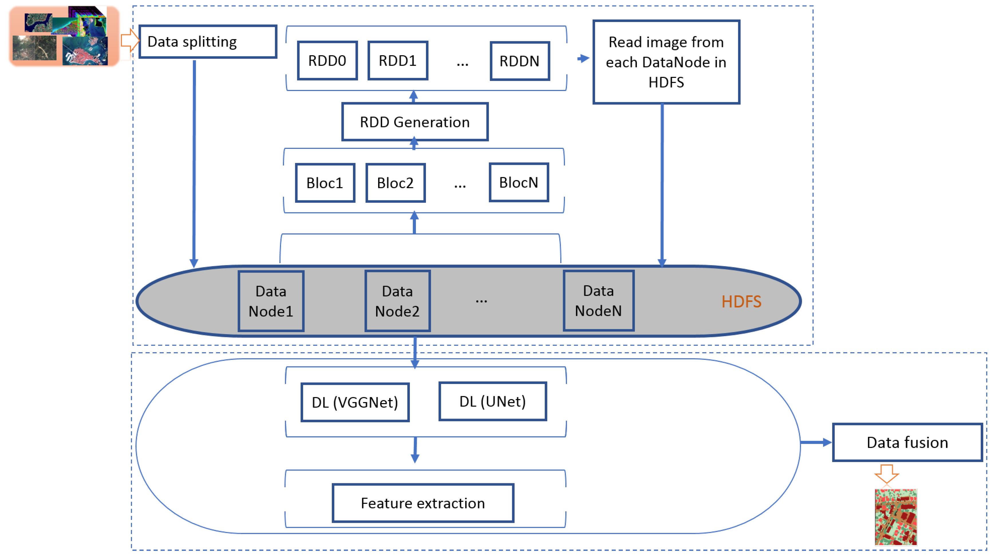
The first step in our approach is the storing phase based on HDFS and Spark-resilient distributed dataset. We begin by loading millions of remote sensing images into HDFS Data Frame.
Those millions of images are considered as BRSD and are characterized by this 4 V:
Volume The amount of data grows in terms of hours and minutes. Between 2017 and 2022, the average data acquisition size could reach 47.7 petabytes per year.
Velocity: Analyze and interpret a large amount of data at a rapidly growing rate.
Veracity refers to bias, noise, and anomaly in the data like uncertainty due to the variety of sources, formats and satellites;
Variety, as remote sensing data can be multi-source, multi-temporal, multi-spectral, or even have multi-resolution. Decoding in the distributed cluster is for large scale manipulation;
After loading the heterogeneous remote sensing data, the first step is to split these images into many parts having the size of 224 × 224. Then every chunk will be duplicated in an HDFS data node of our master–slave architecture.
We store the enormous data in a clustered computer architecture which is a group of computers connected in a common resource pool. This type of architecture is a distributed and parallel system so that we can duplicate all data on all nodes.
Hadoop’s open-source distributed processing software is used in these clusters. One machine in the cluster is usually referred as NameNode, another as JobTracker; these are the masters. The remaining machines in the cluster serve as both DataNode and TaskTracker which are the slaves [
29].
Hadoop and Spark clusters are well known for increasing the speed of data analysis applications. They are also highly scalable: if increasing data volumes exceed a cluster’s processing power, additional cluster nodes can be added to increase throughput. These clusters are terribly proof against failure, as every bit of data is derived to alternative cluster nodes, guaranteeing that data are not lost.
Figure 3 shows the two main categories of machine roles in a Hadoop deployment: master nodes and slave nodes.
The master nodes [
29] are in charge of the two key functional components of Hadoop: storing a large amount of data (HDFS) and performing parallel calculations on all of that data (MapReduce). The node manages and coordinates the data storage function (HDFS), whereas the Job Tracker coordinates and manages parallel data processing using MapReduce. It should be pointed out the use of terms master/slave has been discouraged in the industry and other terms have been proposed as substitution [
29]. This is the focal point and entry point of our architecture. The Spark information coordinator “SparkDriver” distributes tasks uniformly among the executors and receives information from them. Spark’s pilot contains several components, including the Spark’s planning layer, which implements step-by-step planning (DAGScheduler) and TaskScheduler who has in charge of sending tasks to the cluster, executing them, and retrying if they fail, BackendScheduler is in charge of managing multiple server managers. BlockManager is a local cache that runs on each node of the Spark cluster. These components are in charge of converting userSpark code into Spark tasks that are executed on the cluster.
The vast majority of machines are slave nodes [
29], which perform all data storage tasks and performing calculations. Each slave has a data node as well as a Task Tracker daemon that communicates with and receives instructions from their master nodes.
We used the RDD Spark concept to achieve faster and more efficient HDFS operations for storing and MapReduce operation for the second phase of processing. The RDD is a distributed object collection that is immutable. Each RDD data set is divided into logical partitions that are calculated on different cluster nodes.
In order to test this storage method as well as the other methods, we have set up a Hadoop Spark platform which is a distributed computing platform based on the MapReduce and Spark parallel programming model. It has three prerequisites:
The data is divided into small unitary and independent blocks;
The processes must be placed where there is the data (the provision of a large data storage system and allowing to execute code where the data blocks are);
Spark’s fundamental data structure is Resilient Distributed Datasets (RDDs). It is a collection of distributed objects that cannot be changed. Each RDD dataset is divided into logical partitions that are calculated on different cluster nodes.
The basic idea behind Spark is the resilient distributed dataset. RDD supports memory computation. This means that it stores the state of memory as an object in jobs, and the object can be shared between jobs. Data in shared memory is ten to one hundred times faster than network and disk. Therefore, the data are distributed between the various HDFS nodes and the generated RDD nodes.
Once we have blocs of images (224 × 224), we will distribute these images to RDD generated with each image block used to achieve faster and more efficient Map and Reduce operations (shown in
Figure 2) Thus, the first is the matching job, in which our data block is read and processed to produce key-value pairs (ki, vi) as intermediate outputs for the next step. The output of a MAP is in the form of key-value pairs. Then, we will apply the processing phase.
- 2
Processing Phase:
The second phase of our approach is the processing step based on deep learning extraction features presented in
Figure 4. This step of processing is composed of two sub-steps, as we mentioned above, feature extraction and classification are shown in
Figure 4 and explained in next paragraph.
Feature extraction: According to the study of the art of several CNN models for the analysis of BRSD [
16], we chose VGGNet and UNet pre-trained models because they are the most suitable for the processing of our satellite images dataset. The VGGNet model is the most efficient in the processing of RGB images and the UNet model for that of multispectral images.
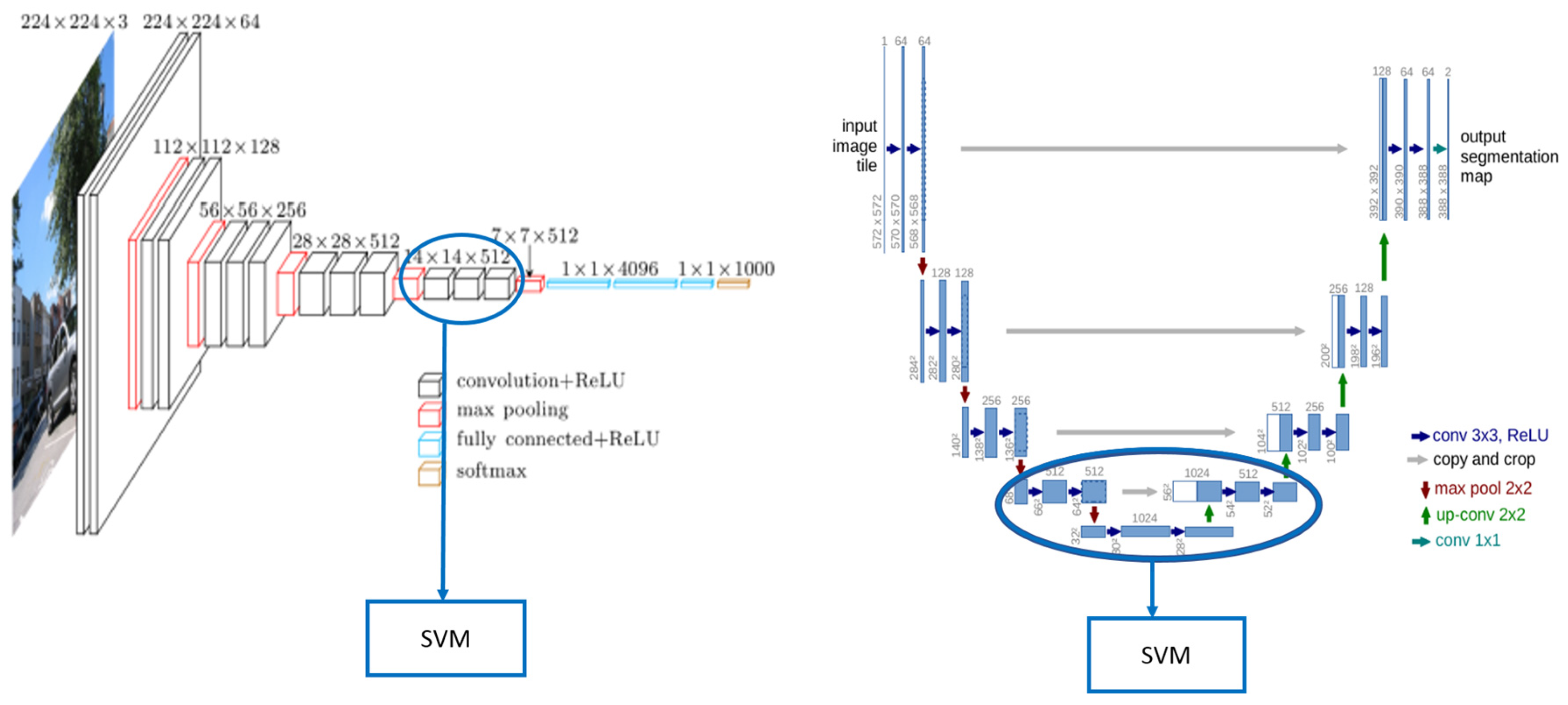
The VGGNet model is a convolutional network that relies on 16 convolutional layers, 13 convolutional layers, and three fully connected layers. The advantage of this architecture is that it consists of two parts: one for the extraction of attributes and the other for the classification knowing that it takes as input an image of size 224 × 224. The processing with VGGNet is applied to the RGB images.
When the output layer of the pre-trained VGGNet-16 is a softmax activation with 1000 classes, we have adapted this layer to 10 classes of softmax layer, which are buildings, cars, crops, fast H2O, roads, slow H2O, structures, tracks, trees, and trucks. As a result, we simply trained the weights of these layers and attempted to recognize the objects.
The UNet model contains 23 convolutional layers distributed between two paths. The encoder is used to capture features in the image. The decoder allows good object recognition. it is a fully convolutional end-to-end network, it contains only convolutional layers and it does not contain fully connected layers. The advantage of this model is it can take as input every type of image. The processing with UNet is applied to the multispectral images.
We trained the model with 90,000 strips of multispectral images and some reactance index, then as the first part of the model is composed of a stack of traditional convolutional layers, we took the features extracted from the bottleneck layer which is considered as our output.
Classification: The two pre-trained model (UNet et VGGNet) were tested first without transfer learning, then with the transfer learning which is based essentially on the transfer of the weights of the different layers which are located: on the three output layers for the VGGNet model and in the encoding block for the UNet model shown in the following
Figure 5.
The output layers for each of the two models have been adapted to incorporate the predefined labels. After the learning phase, we voluntarily disconnect the output layers and we keep the deeper layers under the assumption that these correspond to the features we want to extract. In order to validate this step, we add a classification phase based on the Linear Support Vector Machines (SVM) algorithm whose parameters are the features and the classes are the labels. Linear SVMs have supervised learning models with associated learning algorithms that analyze the data used for classification and regression analysis. In our approach, the purpose of using SVMs is to find a plan that has the maximum margin, which is the maximum distance between the data points of the two classes. Maximizing margin distance for classifying future data points with greater confidence.
The input of our algorithm is then the vector feature of each image chunk that is split. The model of UNet or VGGNet is stored locally in the RDDs after stored in HDFS. The output is a 224 × 224 image that is segmented and classified. Now, as we have the strips of images classified, we will combine them in order to reconstruct the images. After extracting the characteristics and classifying the images, we will now reconstruct them. To perform this step, we will use the second function of MapReduce which is the Reduce. The reducer recieives the key-value pair of the last several tasks, then it includes the intermediate data tuples in a set of tuples, which is the final result. More specifically, the key-value pairs that the reduce phase will receive are the pairs (Kp, Ln) where Ln are the outputs of the classification step, that is, the classified strips of images are going to be grouped in order to reconstruct our images.
The next step is to merge the chunks of images to obtain results as shown in
Figure 4 named data fusion.
Some parts of this second task have been validated in some of our published articles [
30,
31,
32].
Another optional step that has been integrated into the processing phase consists of combining Spark inception V3 and logistic regression in order to compare it with deep learning milestones from ILSVRC (ImageNet Large Scale Visual Recognition Challenge).
Applying the inception V3 model. This model is composed of two main parts which are feature extraction and classification. The feature extraction part is based on Convolutional Neural Networks (CNN) architecture. CNN is one of the deep architectures that are used in DL. In fact, it is a neural network and consists of a trainable multi-layer architecture with convolutional layers, pooling layers, and fully connected layers. The neurons of a single layer are connected to the neurons of the adjacent layers. It showed efficiency in many image domains such as image classification, semantic segmentation, image processing.
CNN can study an image without being affected by translation, scale, rotation, or weight. CNN is efficient in feature extraction using its convolutional and pooling layer. Indeed, CNN is usually composed of more than one feature extraction-stages which represent the convolutional layer that extracts the features through convolving the previous layers. The max-pooling layers take the max pixel value in one region.
For classifying remote sensing images, the CNN architecture involves convolution and max-pooling layers that serve to convert the images to 8 × 8 representations and the average pooling brings these representations to 1 × 1 size. In contrast, the hyperspectral RS scenes classify utilizing the CNN architecture, which involves 1D and 2D the 1D with convolutions in the spectral images and the 2D with the convolutions in the spatial images.
The classification part contains a fully-connected softmax layer. These two layers of output are the final classification result. The fully-connected layer takes the output from the previous layer (S2) as an input and outputs an n-dimensional vector, where n is the number of classes that corresponds to the pixel class.
Transforming images to numeric features using the featurizer which peels off the last layer of a pre-trained neural network and uses the output from all the previous layers as features for the logistic regression algorithm.
The featurizer is based on a machine learning technique called transfer learning. Through this technique, a problem can be solved with stored data that has been stored during other different but related problems. This method is used for a more accurate and fast learning process.
Analyzing independent features with logistic regression using Tensorflow determines the final result.
4. Results
In this section, we present some experimental results in our proposed approach for BRSD to present the performance of the framework proposed in this paper. We begin by describing the system specifications of all the distributed local clusters that are used to implement this approach.
Then we describe the datasets uses for experimentation and our dataset prepared for the validation task.
Table 1 presents the operating system and its characteristics in addition to the frameworks and tools used for our local architecture master/slaves.
To validate the proposed approach, we use three famous remote sensing image datasets which are available for the public, they are collected and acquired from multiple sensors like Landsat-8, Spot-4, Spot-5 and many others. The following
Table 2 presents the characteristics of these datasets as well as our remote sensing imagery dataset that we prepared and collected from many sensors.
The SIRI-WHU dataset [
33] contains 2400 remote sensing images from 12 different classes. Each class contains 200 images with a spatial resolution of 2 m and a resolution of 200 × 200 pixels.
The Intelligent Data Extraction and Analysis of Remote Sensing Group (RSIDEA) at Wuhan University collected it from Google Earth;
The UC Merced land-use dataset [
34] is made up of 2100 overhead scene images divided into 21 land-use scene classes. Each class consists of 100 aerial images measuring 256 × 256 pixels in the red–green–blue color space, with a spatial resolution of 0.3 m per pixel. This dataset was created using aerial ortho imagery obtained from the United States Geological Survey (USGS) National Map;
AID dataset [
35] was created by collecting sample images from Google Earth imagery. As a result, Google Earth images can be used as aerial images to test scene classification algorithms;
Our dataset is composed of 3000 remote sensing images and 10 classes such as buildings, cars, trees, crops, roads, fastH2O, slowH2O, structure, tracks and trucks. The are many images in RGB and others are multispectral; their spatial resolution is between 0.3 m and 3 m.
To validate the proposed approach we used four metrics:
The first metric that we used is the time, in order to evaluate the Speedup (S) present in the following
Table 3 of our architecture comparing to a single node architecture.
The second metric is the precision:
The third metric is the recall:
The fourth metric is the F1-score:
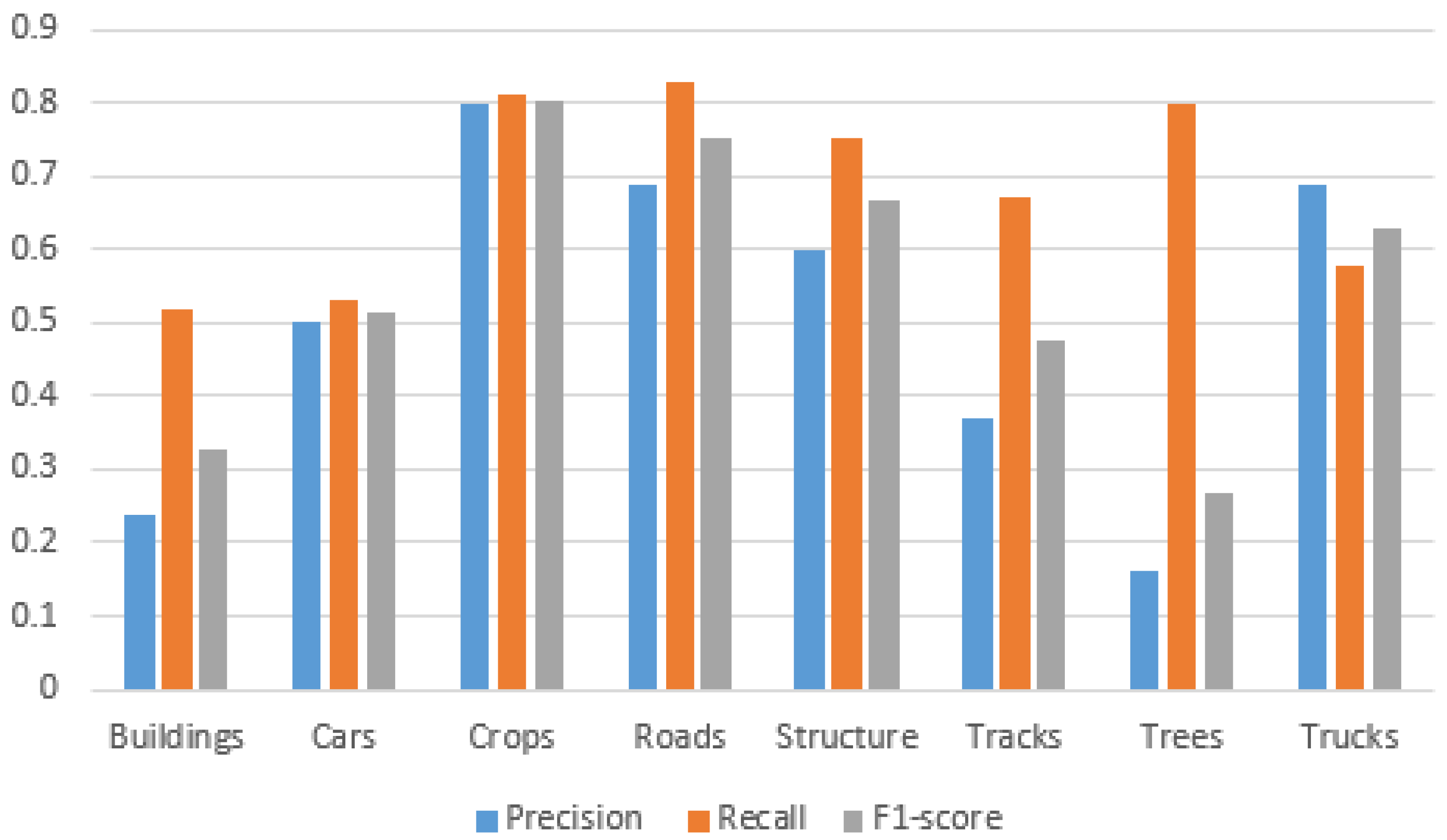
Figure 6,
Figure 7 and
Figure 8 corresponds to the results of the proposed architecture in terms of precision, recall and F-score1 with the VGGNet Model of each label extracted. In addition to an overall comparison between the average error rates for the two models, we compare them on the basis of the classes common to the different datasets. Indeed, in order to have a common benchmark for comparing the efficiency of each model, we present the results of the classification, obtained specifically on the classes in common between the different datasets. The diagrams present the labels in common between the datasets, which are 1-building, 2-cars, 3-crops, 4-roads, 5-structure, 6-tracks, 7-trees, 8-trucks.
The obtained results illustrated in
Figure 9 presented the obtained results of our proposed approach with VGGNet on the three datasets and prove that our approach with the VGGNet model outperforms with our databases and Siri-Whu dataset more than AID dataset.
Now we will presents results with the second deep learning model used which is the UNet model.
Figure 10 corresponds to the results of the proposed architecture on the three datasets and proves that our approach with the UNet model outperforms our databases more than the AID dataset and Siri-Whu dataset.
Figure 11 corresponds to the results of the proposed architecture with the UNet Model of each label extracted on our datasets.
The obtained results after the application of UNET and VGGNet on the SIRI-WHU, were the AID databases, our database and the multispectral images database. The results that we obtained after the application of the UNet model on the images the bases with three bands in term of precision are 84%, 73% and 61%. Applying the UNet model to the 16-band images gave us 94% accuracy. On the other hand, the application on the three-band images gave us an accuracy of 84% at most. The increase in the accuracy rate is due to the nature of the images used for this model which gives additional information on the areas to be predicted.
Some images of our database are shown to illustrate our results.
Figure 12 represents the three-band image results where image (a) is the real RGB image and (b) is the result of our work. We denote that the objects detected in this type of image are impervious surfaces, low vegetation, buildings, cars, trees and clutter.
Figure 13 represents the result of our work on a 16-band image where image (a) indicates the real image scene and (b) is the results that the objects detected in these images which are buildings, cars, crops, fast H2O (rivers, sea), roads, slow H2O (lakes, swimming pool), structures, tracks, trees and trucks.
Table 4 presents the different results obtained in terms of F1-score for our database with the two models pre-trained UNet and VGGNet then the results obtained related to transfer learning For VGGNet-SVM and UNet-SVM.
We have presented the results that we have obtained for the processing of three-band images (RGB images) or for multispectral images. We applied our study on four different databases (three RGB databases and one multispectral image database). We were able to show the added value of transfer learning by comparing the results with and without only on UNet. UNet has been shown to perform better than VGGNet for two major reasons its ability to adapt to multiple resolutions of satellite images and its ability to provide better results.
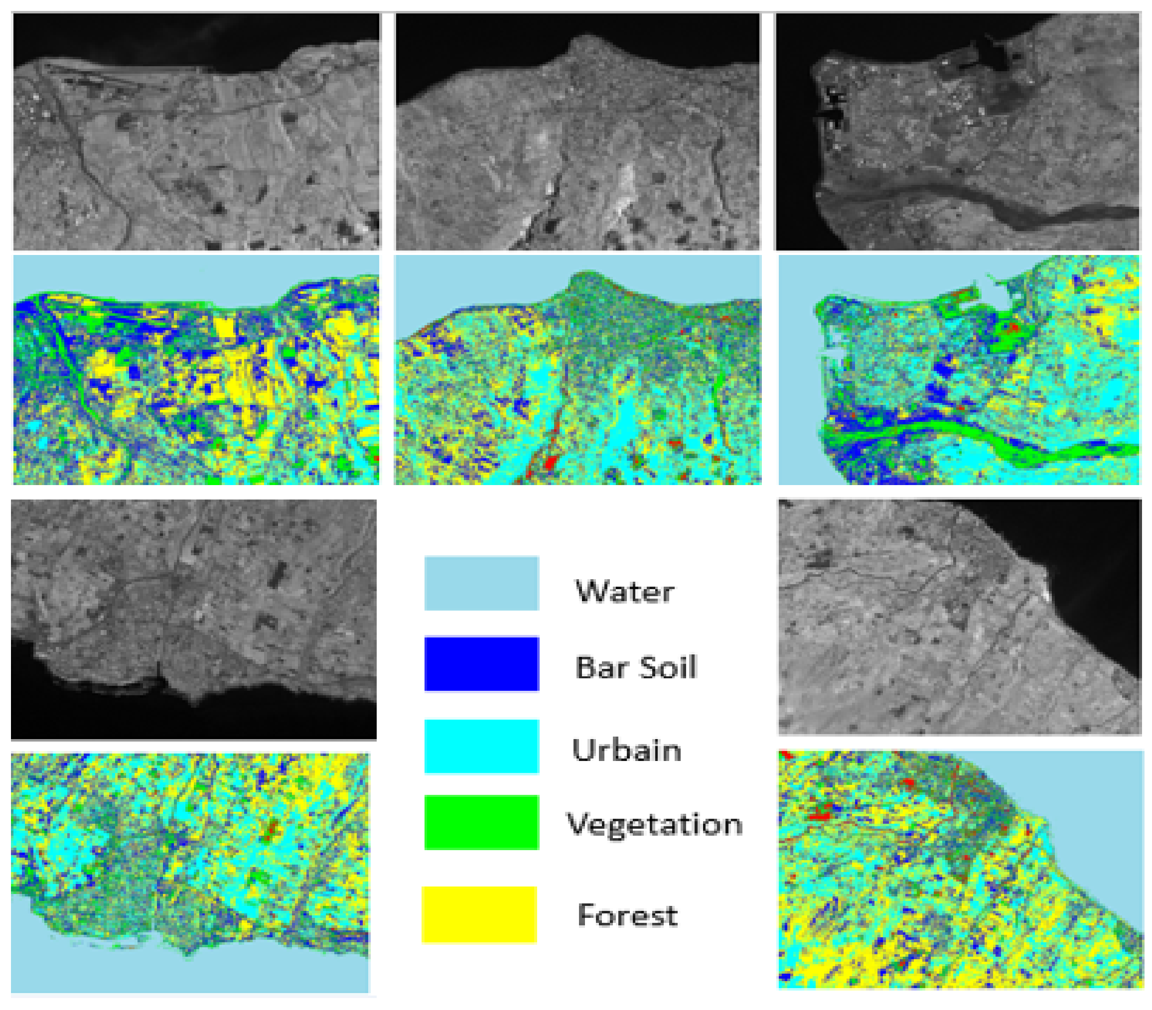
Another type of remote sensing data from our multiple source databases is proposed to validate the proposed approach where we use five experiments’ data which come from SPOT-5 satellite and acquired in 2015 and located in Reunion island. The size of each image is 1.2 GB and each image has been cut into N images in TIFF format (Tagged Image File Format), seven bands and its size is about 60 MB. Results are presented in
Figure 14.
Then we applied the different tasks indicated in the proposed framework which aims to classify our dataset using DL on Spark and Tensorflow by distributing the data distributed and executed parallel processing.
As can be seen from
Table 5, our approach takes full advantage of the entire configuration resources and it makes good results by comparing it to the Google inception V3 model which archives 78.8 accuracies in the ILSVRC 2015.
Discussion
The most common challenge of remote sensing applications are:
ROI (Region of Interest) segmentation and classification;
Few available datasets with labeled images;
Segmentation is a hard task and dependent on image resolution;
Image sizes are higher and higher.
The purpose of our work is to deal with these challenges, and thus to analyze and classify heterogeneous multi-source remote sensing image and to use a parallel distributed architecture coupling two CNN models for feature extraction and labeling. We used a pre-trained DL: VGGNet and UNet for classification and segmentation, they are used as a feature extractor. The use of FCN without a dense layer for that reason can accept images of any size.
We were faced with our approach to standard limitations such as: complex pre-processing which dependent on image scaling and size and complex extracted features, dependent on pre-processing hyperparameters.
We can establish that the reshaping of pre-trained VGGNet can cause a loss of image information. In contrast, the UNet model accepts any image of any size. VGGNet is mainly used for RGB images contrary to UNet which doesn’t impose RGB images as input. So we tested the UNet on the multispectral image as mentioned in the previous results.
5. Conclusions
In this paper, we have proposed an approach for storing and classifying satellite images. The proposed approach is based on a master–slave architecture. It is made up of a master node, several slave nodes and a cluster manager. We have implemented and presented a storage method for massive remote sensing images via Spark and HDFS. In order to classify the images, we used deep learning by integrating the TensorFlow framework with Apache Spark which allows us to process our images pixel by pixel and band by band.
We used the two deep convolutional architectures: the UNet architecture has been best applied to multispectral images (three bands and 20 bands) for feature extraction to improve the classification. The VGGnet architecture has been best applied to rgb images. The final image classification step was performed by SVM algorithms where transfer learning was used to take advantage of deep learning algorithms using the characteristics obtained in the previous step, we succeeded in classifying the images. A benchmark data set of remote sensing images were created for evaluation. Experimental results validated the effectiveness of the proposed approach. In future work, we are going to improve the results and develop other models of deep learning architecture in order to have a framework adapted to each type of remote sensing image.


