Combining Electrostatic, Hindrance and Diffusive Effects for Predicting Particle Transport and Separation Efficiency in Deterministic Lateral Displacement Microfluidic Devices


Abstract
:1. Introduction
2. Phenomenological Aspects of Particle Dynamics and the State of the Art of Modeling Approaches
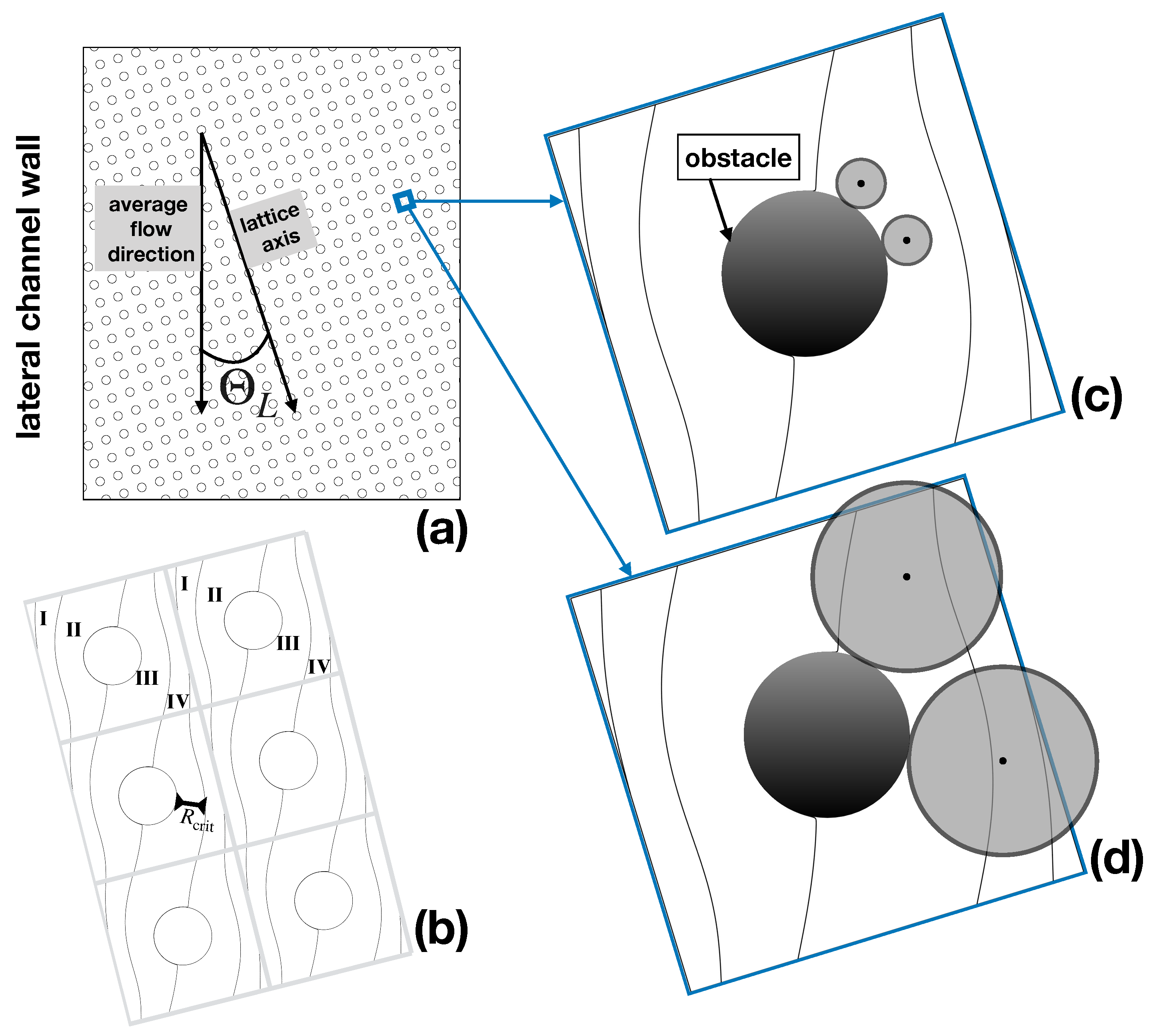
2.1. Phenomenological Aspects of Particle Dynamics
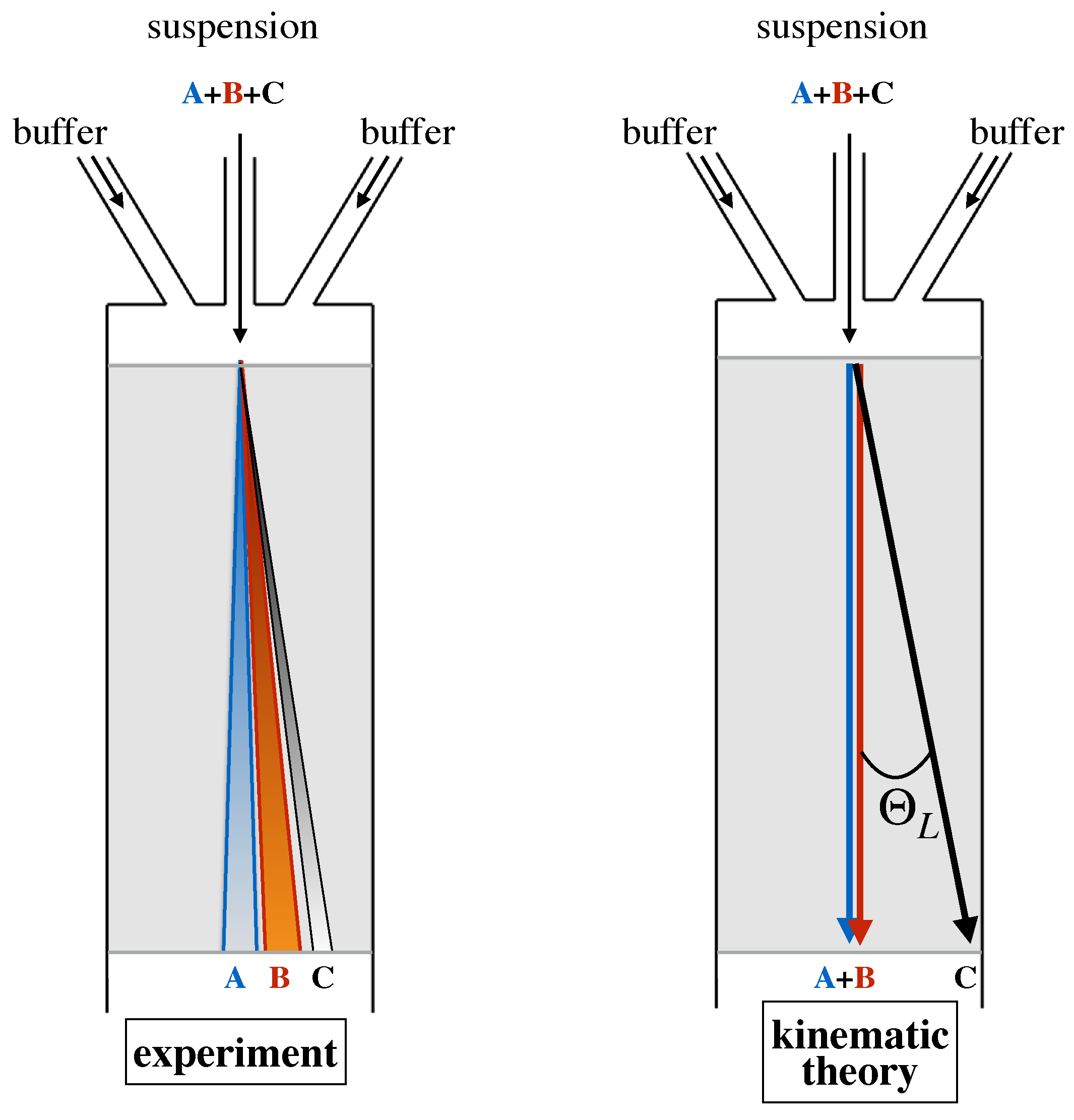
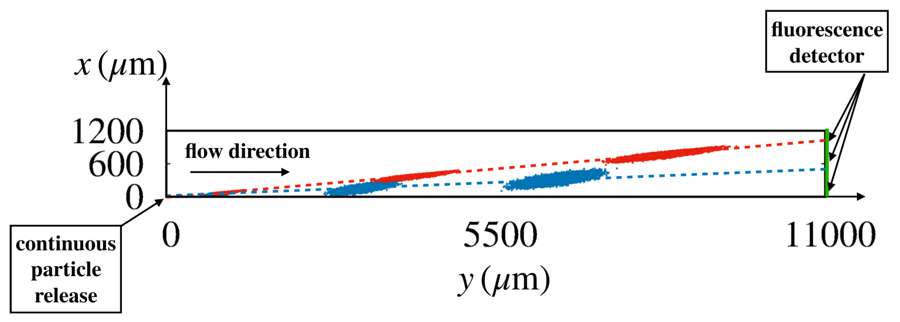
- Even if the inlet stream is focused (i.e., ideally characterized by vanishing thickness) particles of one and the same size tend to scatter transversally to the flow direction as they cross the device, so that they exit the device exit at different positions along the outlet section.
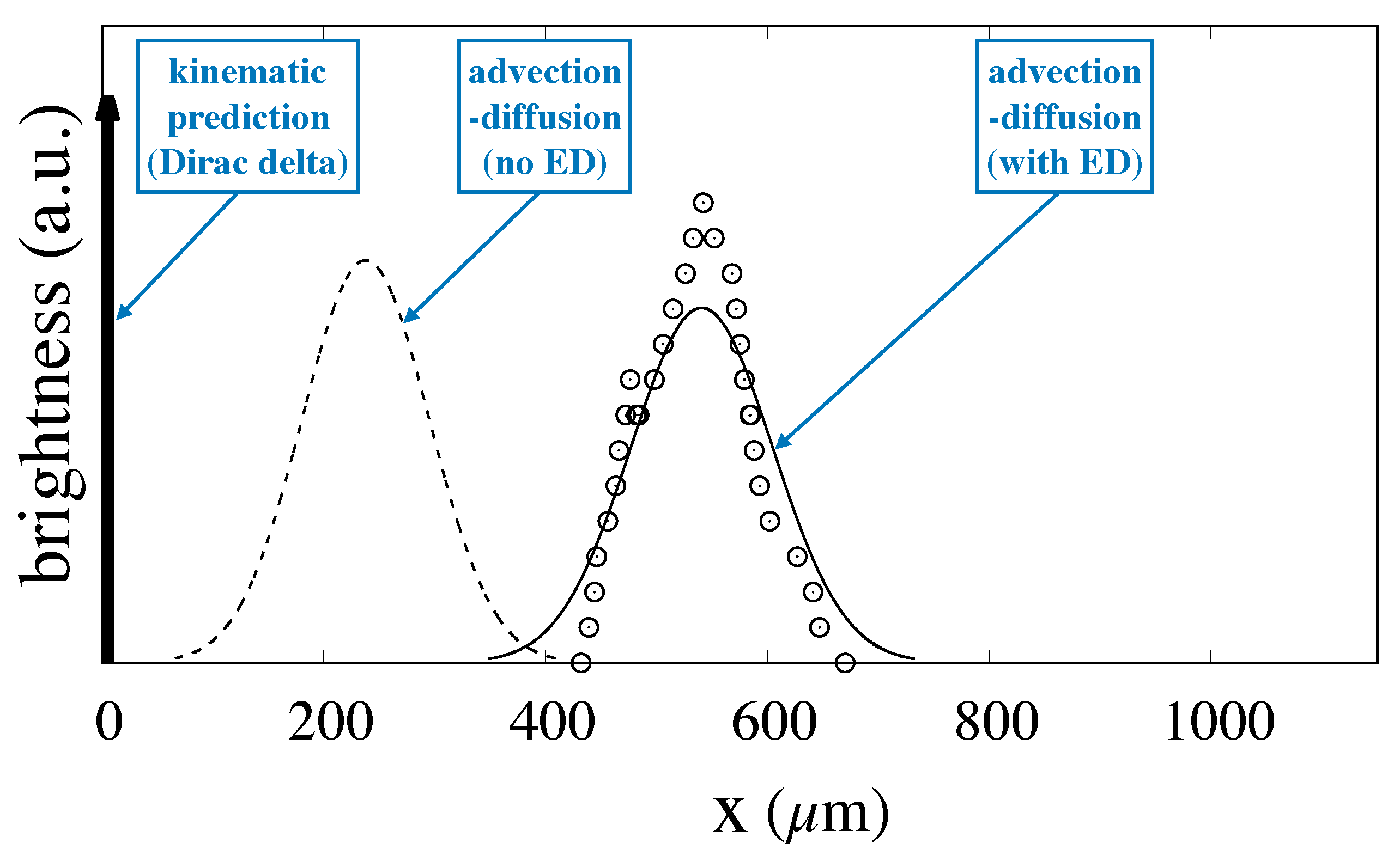
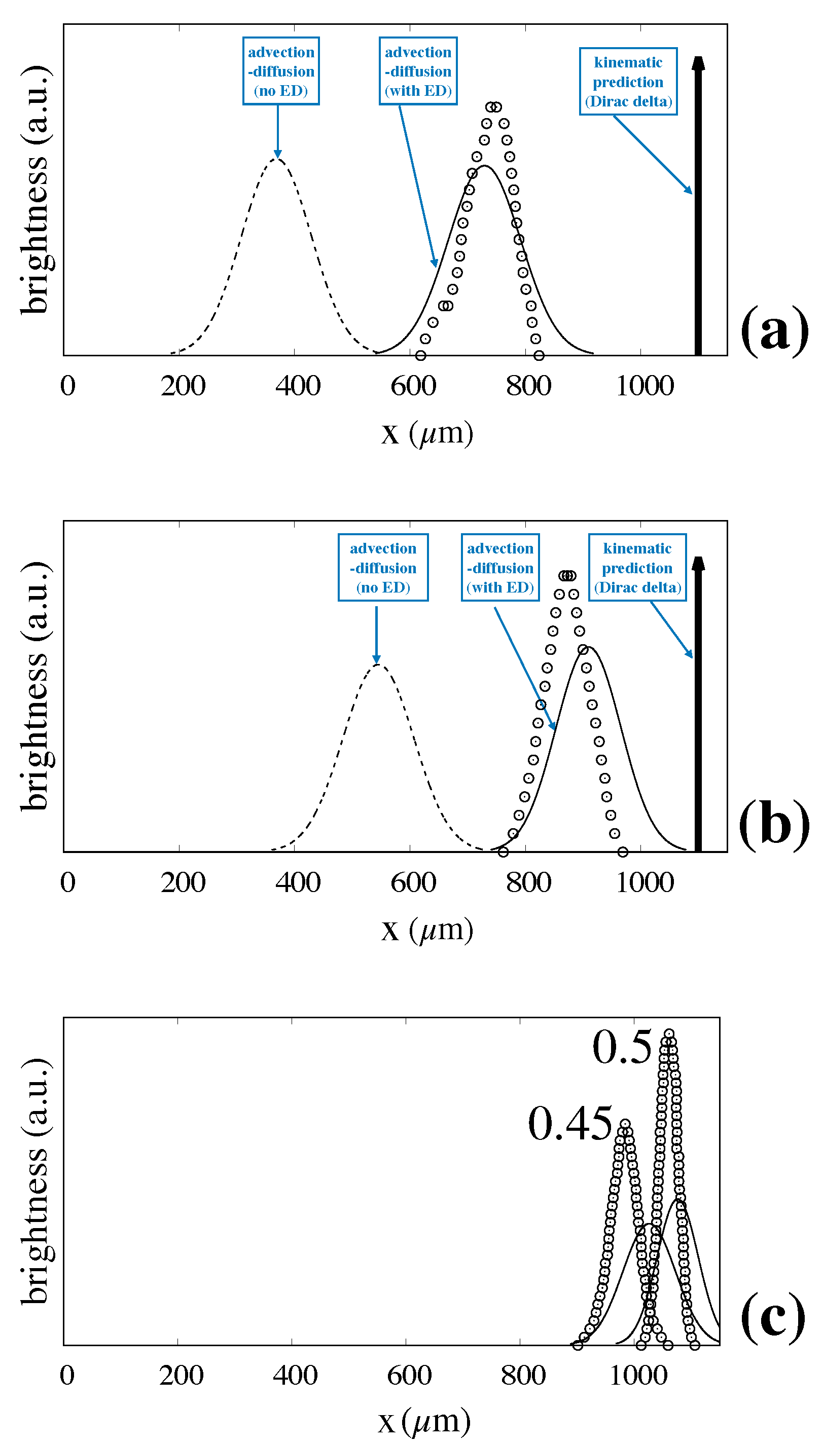
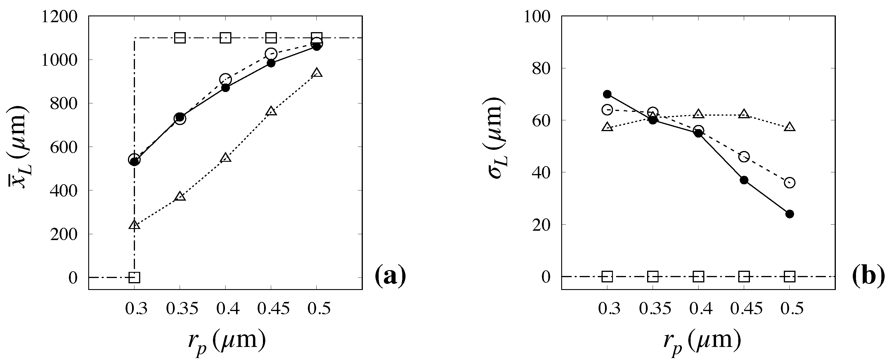
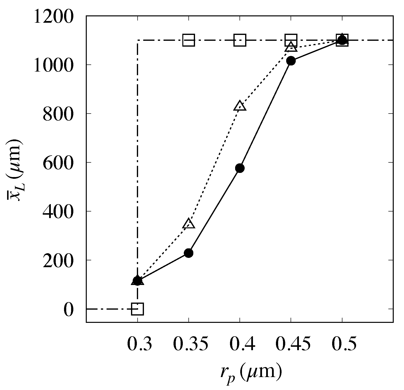
- The average particle deflection (i.e., the median line of each of the particle streams qualitatively depicted in Figure 2 which determines the position of the peak of the distribution at the exit cross-section) depends continuously on particle size, and varies as the flowrate of the suspending solution is varied for one and the same particle size (compare (c) and (d)).
- The dispersion bandwidth about the peak of the exit distribution associated with different particle sizes, which ultimately results from particle diffusion, depends on both the particle size and the flowrate of the suspending solution.
- The comparison between (c) and (d) of Figure 3 shows that the width of the distributions for each particle size is either unaltered or decreases very modestly when the flow rate undergoes a tenfold increase.
- This phenomenon unambiguously indicates the presence of a synergistic effect between the deterministic structure of the flow advecting the particle at the scale of the elementary cell and its isotropic Brownian motion component.
- In fact, in the case where no interaction is assumed between the two transport mechanism (and therefore diffusion could be plainly superimposed to the average particle motion), elementary arguments show that the variance of the distribution should be in the ratio for all particle sizes, which is clearly not the case of the data shown.
2.2. Overdamped (Kinematic) Motion
2.3. Diffusion-Induced Effects
- Two-phase effects, which alter the streamline geometry of the flow and make particle dynamics nontrivial. Such effects are expected to be important for large particles and high flowrates.
- Particle inertia, which makes the particle deviate from the underlying structure of the unperturbed flow. This effect is expected to be significant only at relatively large values of the Reynolds number, a situation that is quite uncommon in practical implementations of the DLD technique.
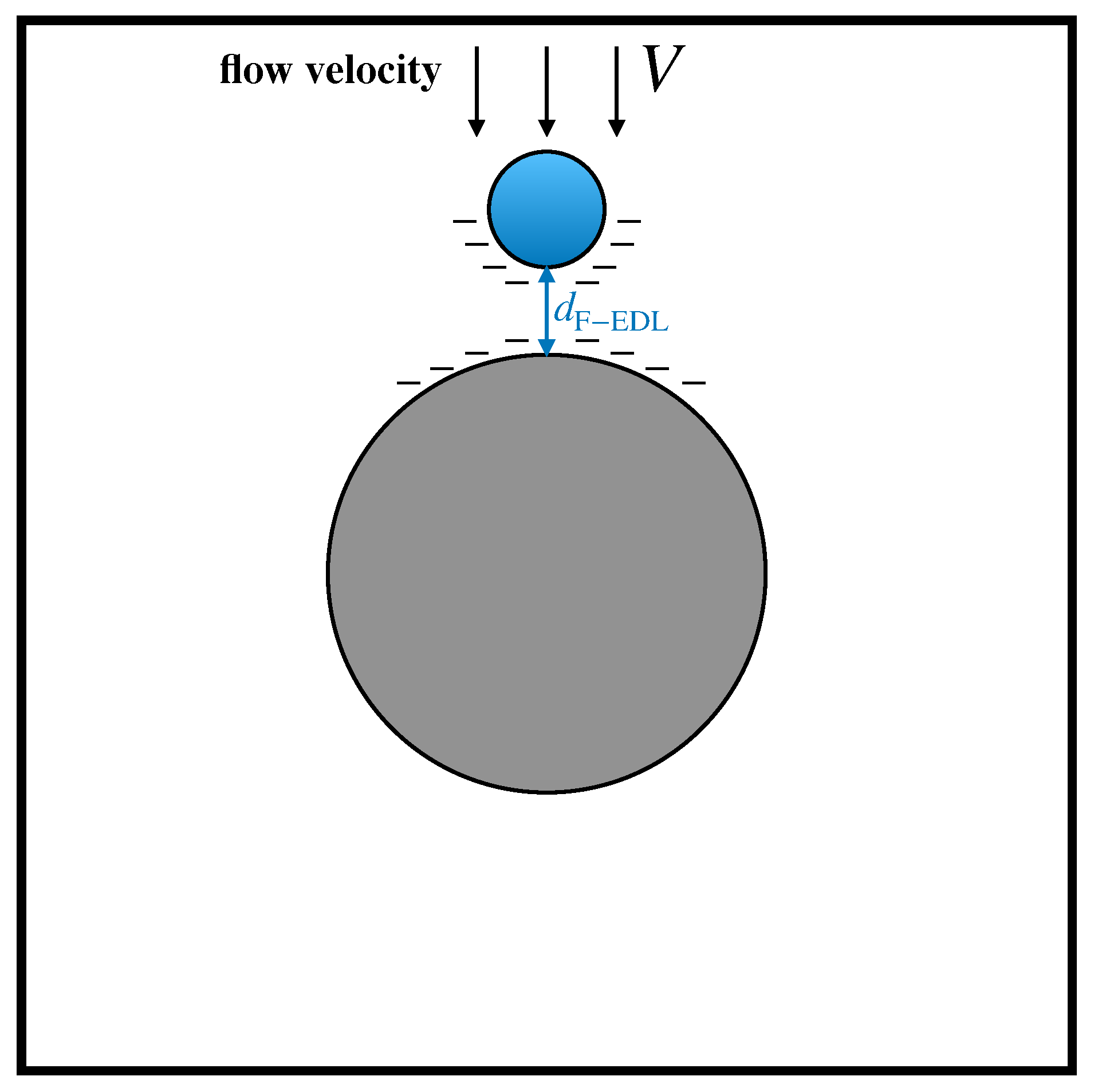
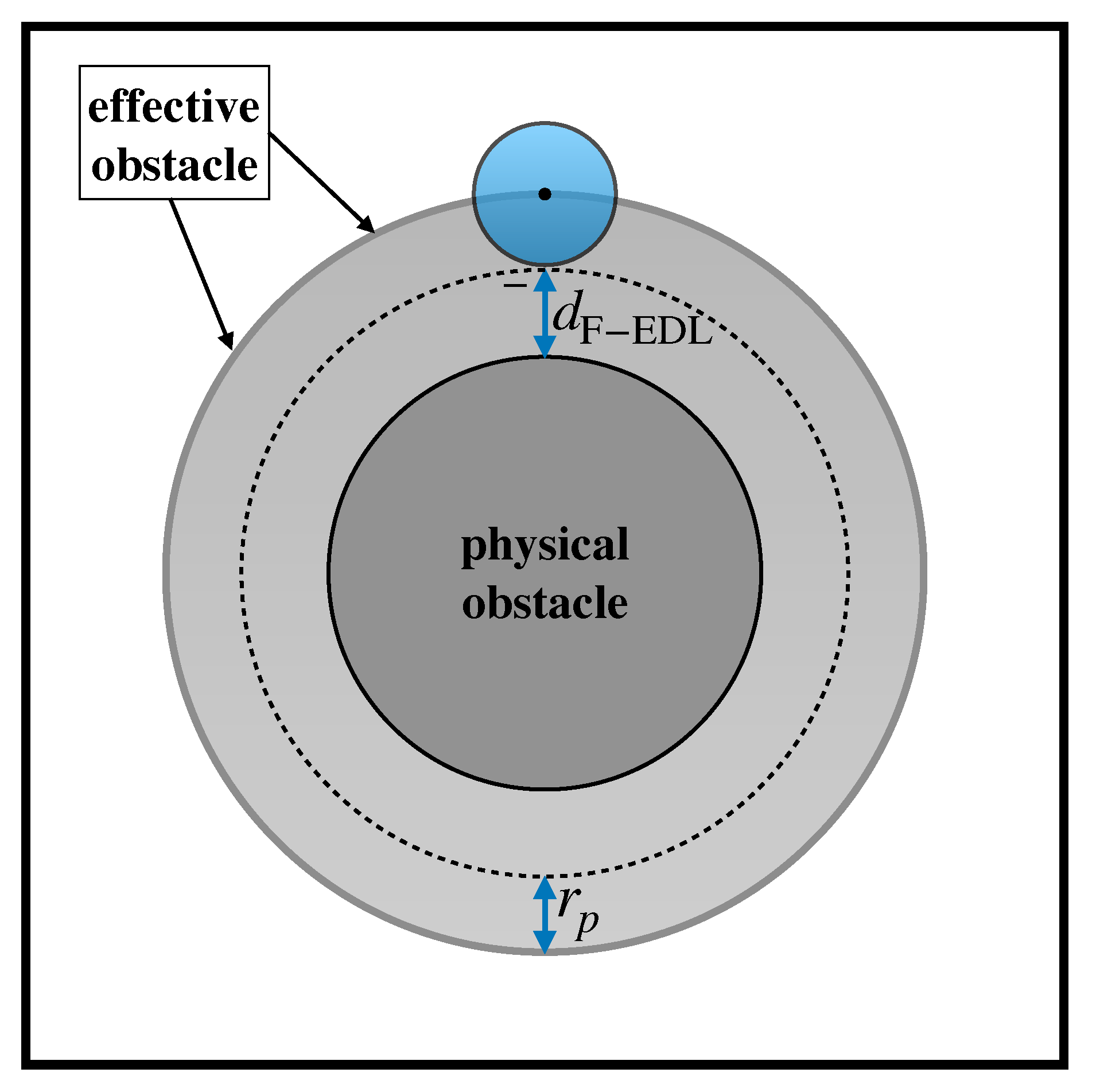
- Surface interactions, which may have an impact on the minimal distance between the particle and the obstacle surface. Note that, in the advection–diffusion model described so far, this distance vanishes during the collision.
2.4. Electrostatic Forces
3. Transport Model and Exit Particle Distributions
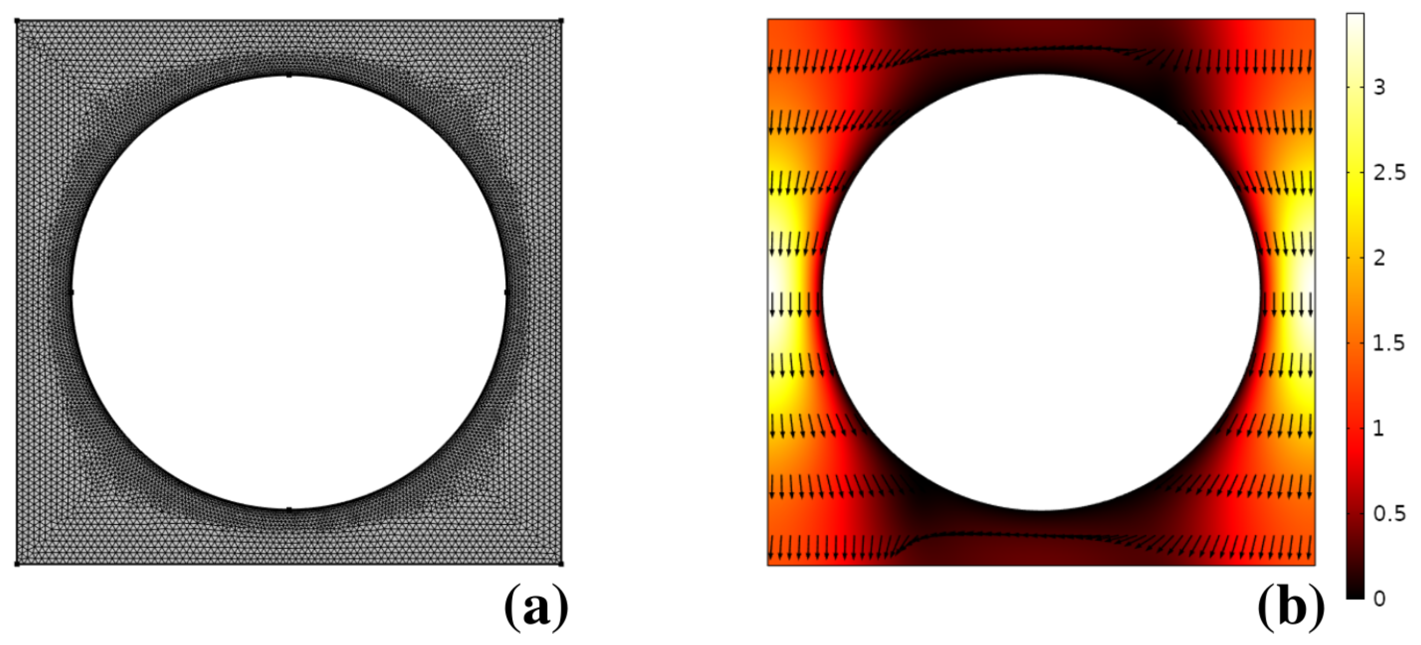
- Compute the single-phase Stokes flow within the unit periodic cell with no slip boundary conditions on the boundary of the physical obstacle and with periodic boundary conditions for the velocity components enforced between the opposite edges of the cell. Because of the presence of the lateral channel walls defining the direction of the average flow, a global constraint on the direction of the average pressure drop must also be enforced (e.g., with reference to Figure 3, and the average pressure drop must be directed along the y-axis).
- Based on the nature of the solid surfaces and the ionic concentration of the buffer solution suspending the particle, compute the surface densities and , and the bare particle diffusivity from the Stokes–Einstein relation. Then, use Equation (4) to compute the electrostatic displacement, and obtain the effective particle radius defined by Equation (5). For a particle of assigned size, the effective particle radius defines the extent of the effective obstacle depicted in Figure 7 and therefore the region accessible to the center of the particle.
- Initialize the position of the center of the particle at the release point (here the origin of the coordinate system), and use Equation (2) to advance this position in time for a (small) finite interval . Because the solution of the velocity field is obtained numerically, an interpolation scheme is necessary for computing at a generic position .
- If the advanced position falls beyond the boundary of the effective obstacle, reflect the portion of the displacement vector that falls within the boundary about the local normal vector.
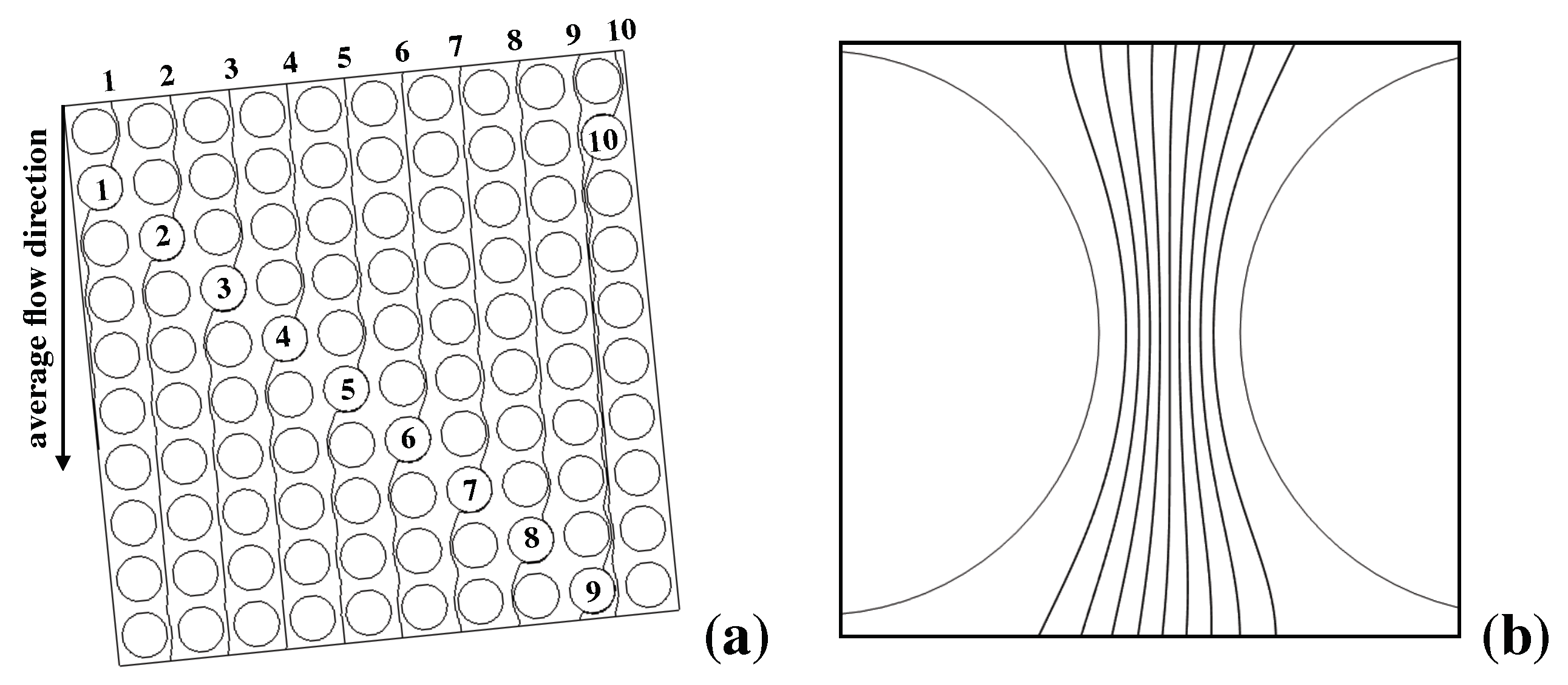
- Repeat the integration for a large number of independent realizations, say , of the stochastic process to obtain the evolution of the ensemble of trajectories as those depicted in Figure 5.
- Define the ensemble-average operatorof an observable s evolving alongside a generic realization of the stochastic process. Track the first and second moments of the ensemble, , , and . After a short transient, the first moments and the squared variance of the ensemble display a linear time scaling,Here, and physically represent the center of mass of the ensemble. Thus, by tracking , , the the effective velocity and the entry of the (symmetric) effective dispersion tensor can be computed from the ensemble dynamics by linear regression.
- From the effective transport coefficients, the peak position, and the variance entering the steady-state Gaussian distribution in Equation (3) can be computed asandWe note that the expression of the variance given by Equation (10) constitutes an approximation in that the continuous effective dispersion coefficient as defined in [30] should appear on the right-hand side in place of . However, in all of the cases where the lattice angle is small (which is largely verified in practical implementations of the separation method), one finds that , so that Equation (10) holds true.
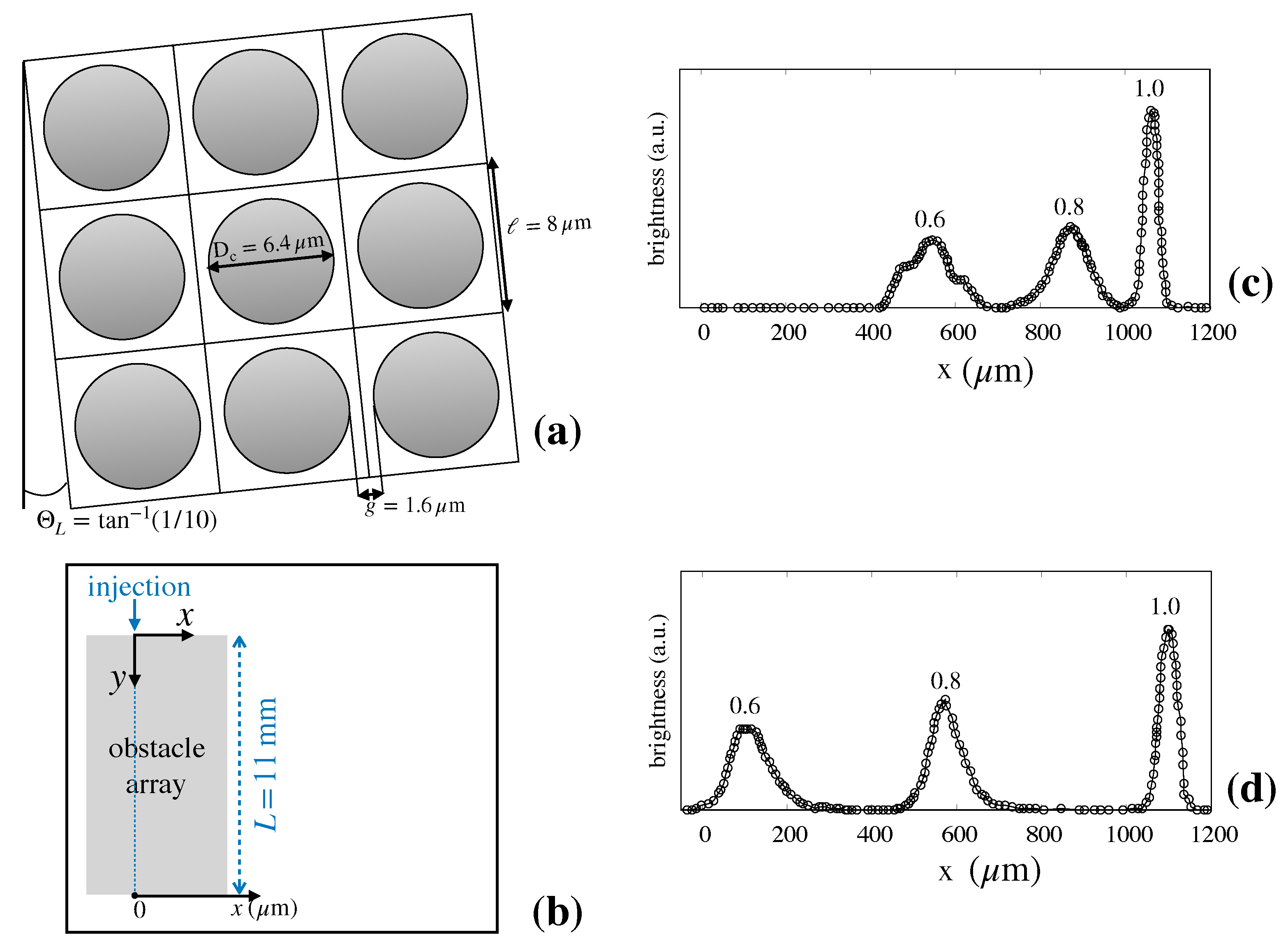
4. Case Study
5. Conclusions
Author Contributions
Funding
Acknowledgments
Conflicts of Interest
References
- Dincau, B.M.; Lee, Y.; Kim, J.H.; Yeo, W.H. Recent advances in nanoparticle concentration and their application in viral detection using integrated sensors. Sensors 2017, 17, 2316. [Google Scholar] [CrossRef] [Green Version]
- Jungbauer, A. Continuous downstream processing of biopharmaceuticals. Trends Biotechnol. 2013, 31, 479–492. [Google Scholar] [CrossRef] [PubMed]
- Hong, P.; Koza, S.; Bouvier, E.S. A review size-exclusion chromatography for the analysis of protein biotherapeutics and their aggregates. J. Liq. Chromatogr. Relat. Technol. 2012, 35, 2923–2950. [Google Scholar] [PubMed] [Green Version]
- Striegel, A.M.; Brewer, A.K. Hydrodynamic chromatography. Annu. Rev. Anal. Chem. 2012, 5, 15–34. [Google Scholar] [CrossRef] [PubMed]
- Small, H.; Lanshorst, M. Hydrodynamic chromatography. Anal. Chem. 1982, 54, 892A–898A. [Google Scholar] [CrossRef]
- Huang, L.; Cox, E.; Austin, R.; Sturm, J. Continuous particle separation through deterministic lateral displacement. Science 2004, 304, 987–990. [Google Scholar] [CrossRef]
- Adrover, A.; Cerbelli, S. Laminar dispersion at low and high Peclet numbers in finite-length patterned microtubes. Phys. Fluids 2017, 29, 062005. [Google Scholar] [CrossRef]
- Adrover, A.; Cerbelli, S.; Giona, M. Taming axial dispersion in hydrodynamic chromatography columns through wall patterning. Phys. Fluids 2018, 30, 042002. [Google Scholar] [CrossRef]
- Hochstetter, A.; Vernekar, R.; Austin, R.H.; Becker, H.; Beech, J.P.; Fedosov, D.A.; Gompper, G.; Kim, S.C.; Smith, J.T.; Stolovitzky, G.; et al. Deterministic Lateral Displacement: Challenges and Perspectives. ACS Nano 2020. [Google Scholar] [CrossRef] [PubMed]
- Salafi, T.; Zhang, Y.; Zhang, Y. A review on deterministic lateral displacement for particle separation and detection. Nano-Micro Lett. 2019, 11, 77. [Google Scholar] [CrossRef] [Green Version]
- Inglis, D.W.; Lord, M.; Nordon, R.E. Scaling deterministic lateral displacement arrays for high throughput and dilution-free enrichment of leukocytes. J. Micromech. Microeng. 2011, 21, 054024. [Google Scholar] [CrossRef]
- Loutherback, K.; D’Silva, J.; Liu, L.; Wu, A.; Austin, R.H.; Sturm, J.C. Deterministic separation of cancer cells from blood at 10 mL/min. AIP Adv. 2012, 2, 042107. [Google Scholar] [CrossRef] [PubMed] [Green Version]
- Okano, H.; Konishi, T.; Suzuki, T.; Suzuki, T.; Ariyasu, S.; Aoki, S.; Abe, R.; Hayase, M. Enrichment of circulating tumor cells in tumor-bearing mouse blood by a deterministic lateral displacement microfluidic device. Biomed. Microdevices 2015, 17, 59. [Google Scholar] [CrossRef] [PubMed]
- Liu, Z.; Huang, F.; Du, J.; Shu, W.; Feng, H.; Xu, X.; Chen, Y. Rapid isolation of cancer cells using microfluidic deterministic lateral displacement structure. Biomicrofluidics 2013, 7, 011801. [Google Scholar] [CrossRef] [PubMed]
- Liu, Z.; Zhang, W.; Huang, F.; Feng, H.; Shu, W.; Xu, X.; Chen, Y. High throughput capture of circulating tumor cells using an integrated microfluidic system. Biosens. Bioelectron. 2013, 47, 113–119. [Google Scholar] [CrossRef]
- Wunsch, B.H.; Kim, S.C.; Gifford, S.M.; Astier, Y.; Wang, C.; Bruce, R.L.; Patel, J.V.; Duch, E.A.; Dawes, S.; Stolovitzky, G.; et al. Gel-on-a-chip: Continuous, velocity-dependent DNA separation using nanoscale lateral displacement. Lab Chip 2019, 19, 1567–1578. [Google Scholar] [CrossRef]
- Wunsch, B.H.; Smith, J.T.; Gifford, S.M.; Wang, C.; Brink, M.; Bruce, R.L.; Austin, R.H.; Stolovitzky, G.; Astier, Y. Nanoscale lateral displacement arrays for the separation of exosomes and colloids down to 20 nm. Nat. Nanotechnol. 2016, 11, 936–940. [Google Scholar] [CrossRef]
- Inglis, D.; Herman, N.; Vesey, G. Highly accurate deterministic lateral displacement device and its application to purification of fungal spores. Biomicrofluidics 2010, 4, 8–9. [Google Scholar] [CrossRef] [Green Version]
- Holm, S.; Beech, J.; Barrett, M.; Tegenfeldt, J. Separation of parasites from human blood using deterministic lateral displacement. Lab Chip Miniaturisation Chem. Biol. 2011, 11, 1326–1332. [Google Scholar] [CrossRef]
- Green, J.; Radisic, M.; Murthy, S. Deterministic lateral displacement as a means to enrich large cells for tissue engineering. Anal. Chem. 2009, 81, 9178–9182. [Google Scholar] [CrossRef]
- Davis, J.A.; Inglis, D.W.; Morton, K.J.; Lawrence, D.A.; Huang, L.R.; Chou, S.Y.; Sturm, J.C.; Austin, R.H. Deterministic hydrodynamics: Taking blood apart. Proc. Natl. Acad. Sci. USA 2006, 103, 14779–14784. [Google Scholar] [CrossRef] [PubMed] [Green Version]
- Hou, H.W.; Bhagat, A.A.S.; Lee, W.C.; Huang, S.; Han, J.; Lim, C.T. Microfluidic devices for blood fractionation. Micromachines 2011, 2, 319–343. [Google Scholar] [CrossRef] [Green Version]
- Loutherback, K.; Chou, K.S.; Newman, J.; Puchalla, J.; Austin, R.H.; Sturm, J.C. Improved performance of deterministic lateral displacement arrays with triangular posts. Microfluid. Nanofluidics 2010, 9, 1143–1149. [Google Scholar] [CrossRef]
- Zeming, K.K.; Ranjan, S.; Zhang, Y. Rotational separation of non-spherical bioparticles using I-shaped pillar arrays in a microfluidic device. Nat. Commun. 2013, 4, 1625. [Google Scholar] [CrossRef] [PubMed] [Green Version]
- Brenner, H.; Edwards, D. Macrotransport Processes; Butterworth-Heinemann Series in Chemical Engineering; Elsevier: Amsterdam, The Netherlands, 1993. [Google Scholar]
- Majda, A.J.; Kramer, P.R. Simplified models for turbulent diffusion: Theory, numerical modelling, and physical phenomena. Phys. Rep. 1999, 314, 237–574. [Google Scholar] [CrossRef]
- Heller, M.; Bruus, H. A theoretical analysis of the resolution due to diffusion and size dispersion of particles in deterministic lateral displacement devices. J. Micromech. Microeng. 2008, 18, 075030. [Google Scholar] [CrossRef]
- Cerbelli, S. Separation of polydisperse particle mixtures by deterministic lateral displacement. the impact of particle diffusivity on separation efficiency. Asia Pac. J. Chem. Eng. 2012, 7, S356–S371. [Google Scholar] [CrossRef]
- Cerbelli, S.; Giona, M.; Garofalo, F. Quantifying dispersion of finite-sized particles in deterministic lateral displacement microflow separators through Brenner’s macrotransport paradigm. Microfluid. Nanofluidics 2013, 15, 431–449. [Google Scholar] [CrossRef]
- Cerbelli, S.; Garofalo, F.; Giona, M. Effective dispersion and separation resolution in continuous particle fractionation. Microfluid. Nanofluidics 2015, 19, 1035–1046. [Google Scholar] [CrossRef]
- Giona, M.; Brasiello, A.; Crescitelli, S. Ergodicity-breaking bifurcations and tunneling in hyperbolic transport models. EPL Europhys. Lett. 2015, 112, 30001. [Google Scholar] [CrossRef]
- Krüger, T.; Holmes, D.; Coveney, P.V. Deformability-based red blood cell separation in deterministic lateral displacement devices—A simulation study. Biomicrofluidics 2014, 8, 054114. [Google Scholar] [PubMed] [Green Version]
- Zeming, K.K.; Thakor, N.V.; Zhang, Y.; Chen, C.H. Real-time modulated nanoparticle separation with an ultra-large dynamic range. Lab Chip 2016, 16, 75–85. [Google Scholar] [PubMed]
- Zeming, K.K.; Salafi, T.; Shikha, S.; Zhang, Y. Fluorescent label-free quantitative detection of nano-sized bioparticles using a pillar array. Nat. Commun. 2018, 9, 1–10. [Google Scholar]
- Kim, S.; Karrila, S.J. Microhydrodynamics: Principles and Selected Applications; Butterworth-Heinemann Series in Chemical Engineering; Courier Corporation: North Chelmsford, MA, USA, 1991. [Google Scholar]
- Biagioni, V.; Adrover, A.; Cerbelli, S. On the three-dimensional structure of the flow through deterministic lateral displacement devices and its effects on particle separation. Processes 2019, 7, 498. [Google Scholar]


© 2020 by the authors. Licensee MDPI, Basel, Switzerland. This article is an open access article distributed under the terms and conditions of the Creative Commons Attribution (CC BY) license (http://creativecommons.org/licenses/by/4.0/).
Share and Cite
Biagioni, V.; Balestrieri, G.; Adrover, A.; Cerbelli, S. Combining Electrostatic, Hindrance and Diffusive Effects for Predicting Particle Transport and Separation Efficiency in Deterministic Lateral Displacement Microfluidic Devices. Biosensors 2020, 10, 126. https://0-doi-org.brum.beds.ac.uk/10.3390/bios10090126
Biagioni V, Balestrieri G, Adrover A, Cerbelli S. Combining Electrostatic, Hindrance and Diffusive Effects for Predicting Particle Transport and Separation Efficiency in Deterministic Lateral Displacement Microfluidic Devices. Biosensors. 2020; 10(9):126. https://0-doi-org.brum.beds.ac.uk/10.3390/bios10090126
Chicago/Turabian StyleBiagioni, Valentina, Giulia Balestrieri, Alessandra Adrover, and Stefano Cerbelli. 2020. "Combining Electrostatic, Hindrance and Diffusive Effects for Predicting Particle Transport and Separation Efficiency in Deterministic Lateral Displacement Microfluidic Devices" Biosensors 10, no. 9: 126. https://0-doi-org.brum.beds.ac.uk/10.3390/bios10090126