
CT in the Differentiation of Gliomas from Brain Metastases: The Radiomics Analysis of the Peritumoral Zone


 , , and
Abstract
:1. Introduction
2. Materials and Methods
2.1. Patients
2.2. Reference Standard
2.3. Image Acquisition and Interpretation
2.4. Texture Analysis
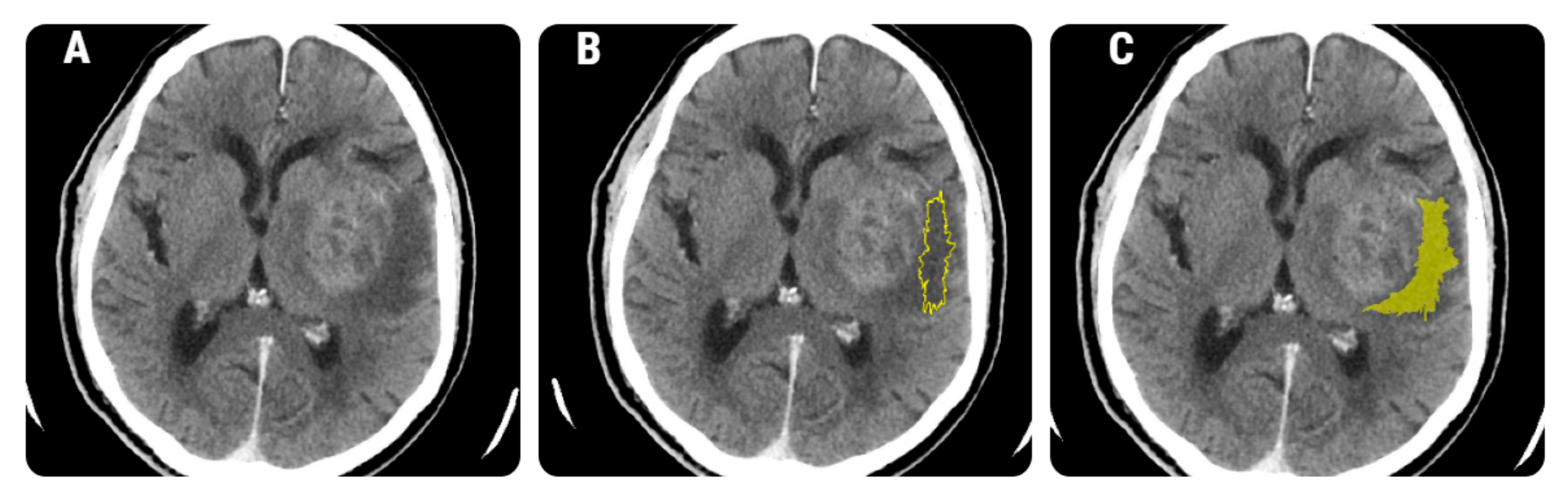
2.4.1. Image Pre-Processing and Segmentation
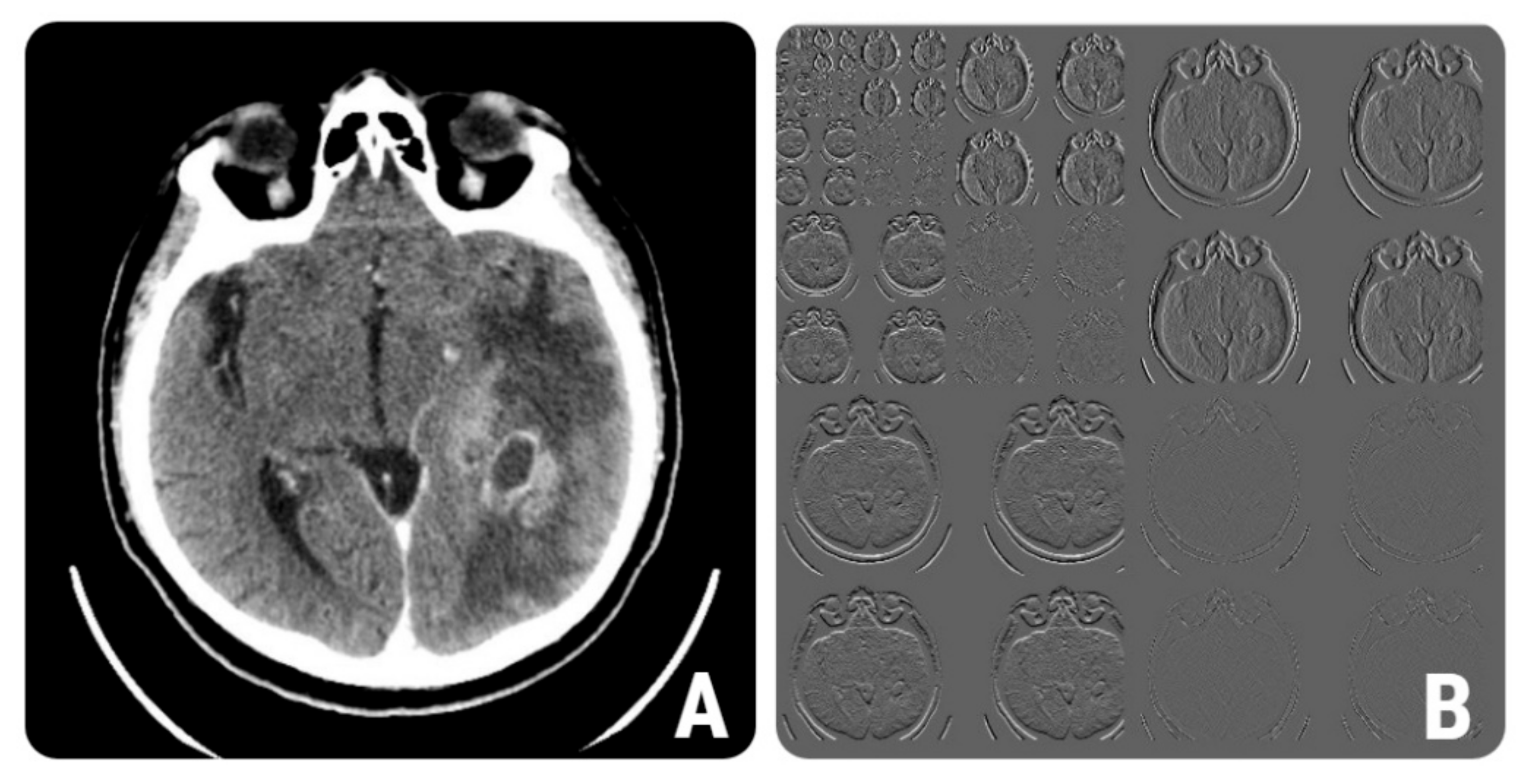
2.4.2. Feature Extraction
2.4.3. Feature Selection
2.4.4. Class Prediction
3. Results
4. Discussion
5. Conclusions
Author Contributions
Funding
Institutional Review Board Statement
Informed Consent Statement
Data Availability Statement
Conflicts of Interest
References
- Giese, A.; Westphal, M. Treatment of malignant glioma: A problem beyond the margins of resection. J. Cancer Res. Clin. Oncol. 2001, 127, 217–225. [Google Scholar] [CrossRef]
- Montemurro, N.; Fanelli, G.N.; Scatena, C.; Ortenzi, V.; Pasqualetti, F.; Mazzanti, C.M.; Morganti, R.; Paiar, F.; Naccarato, A.G.; Perrini, P. Surgical outcome and molecular pattern characterization of recurrent glioblastoma multiforme: A single-center retrospective series. Clin. Neurol. Neurosurg. 2021, 207, 106735. [Google Scholar] [CrossRef]
- Sivasanker, M.; Madhugiri, V.S.; Moiyadi, A.V.; Shetty, P.; Subi, T.S. Surgery for brain metastases: An analysis of outcomes and factors affecting survival. Clin. Neurol. Neurosurg. 2018, 168, 153–162. [Google Scholar] [CrossRef]
- Byrnes, T.J.D.; Barrick, T.R.; Bell, B.A.; Clark, C.A. Diffusion tensor imaging discriminates between glioblastoma and cerebral metastasesin vivo. NMR Biomed. 2011, 24, 54–60. [Google Scholar] [CrossRef]
- Blanchet, L.; Krooshof, P.; Postma, G.; Idema, A.; Goraj, B.; Heerschap, A.; Buydens, L. Discrimination between Metastasis and Glioblastoma Multiforme Based on Morphometric Analysis of MR Images. Am. J. Neuroradiol. 2010, 32, 67–73. [Google Scholar] [CrossRef] [PubMed] [Green Version]
- Lemée, J.-M.; Clavreul, A.; Menei, P. Intratumoral heterogeneity in glioblastoma: Don’t forget the peritumoral brain zone. Neuro-Oncology 2015, 17, 1322–1332. [Google Scholar] [CrossRef]
- Aubry, M.; De Tayrac, M.; Etcheverry, A.; Clavreul, A.; Saikali, S.; Menei, P.; Mosser, J. From the core to beyond the margin: A genomic picture of glioblastoma intratumor heterogeneity. Oncotarget 2015, 6, 12094–12109. [Google Scholar] [CrossRef] [Green Version]
- Lee, E.J.; Terbrugge, K.; Mikulis, D.; Choi, D.S.; Bae, J.M.; Lee, S.K.; Moon, S.Y. Diagnostic Value of Peritumoral Minimum Apparent Diffusion Coefficient for Differentiation of Glioblastoma Multiforme From Solitary Metastatic Lesions. Am. J. Roentgenol. 2011, 196, 71–76. [Google Scholar] [CrossRef] [PubMed]
- Wang, W.; Steward, C.; Desmond, P. Diffusion Tensor Imaging in Glioblastoma Multiforme and Brain Metastases: The Role of p, q, L, and Fractional Anisotropy. Am. J. Neuroradiol. 2009, 30, 203–208. [Google Scholar] [CrossRef] [Green Version]
- Neves, S.; Mazal, P.; Wanschitz, J.; Rudnay, A.C.; Drlicek, M.; Czech, T.; Wüstinger, C.; Budka, H. Pseudogliomatous growth pattern of anaplastic small cell carcinomas metastatic to the brain. Clin. Neuropathol. 2001, 20, 38–42. [Google Scholar]
- Van Timmeren, J.E.; Cester, D.; Tanadini-Lang, S.; Alkadhi, H.; Baessler, B. Radiomics in medical imaging—“how-to” guide and critical reflection. Insights Imaging 2020, 11, 91. [Google Scholar] [CrossRef]
- Mannil, M.; Von Spiczak, J.; Manka, R.; Alkadhi, H. Texture Analysis and Machine Learning for Detecting Myocardial Infarction in Noncontrast Low-Dose Computed Tomography. Investig. Radiol. 2018, 53, 338–343. [Google Scholar] [CrossRef] [PubMed]
- Gadkari, D. Image Quality Analysis Using GLCM. Master’s Thesis, University of Central Florida, Orlando, FL, USA, 2004. [Google Scholar]
- Larroza, A.; Bodí, V.; Moratal, D. Texture Analysis in Magnetic Resonance Imaging: Review and Considerations for Future Applications. In Assessment of Cellular and Organ Function and Dysfunction Using Direct and Derived MRI Methodologies; IntechOpen: London, UK, 2016. [Google Scholar]
- Lubner, M.G.; Smith, A.D.; Sandrasegaran, K.; Sahani, D.V.; Pickhardt, P.J. CT Texture Analysis: Definitions, Applications, Biologic Correlates, and Challenges. Radiographics 2017, 37, 1483–1503. [Google Scholar] [CrossRef] [PubMed]
- Kang, Y.; Choi, S.H.; Kim, Y.-J.; Kim, K.G.; Sohn, C.-H.; Kim, J.-H.; Yun, T.J.; Chang, K.-H. Gliomas: Histogram Analysis of Apparent Diffusion Coefficient Maps with Standard- or High-b-Value Diffusion-weighted MR Imaging—Correlation with Tumor Grade. Radiology 2011, 261, 882–890. [Google Scholar] [CrossRef] [PubMed] [Green Version]
- Raja, R.; Sinha, N.; Saini, J.; Mahadevan, A.; Rao, K.N.; Swaminathan, A. Assessment of tissue heterogeneity using diffusion tensor and diffusion kurtosis imaging for grading gliomas. Neuroradiology 2016, 58, 1217–1231. [Google Scholar] [CrossRef] [PubMed]
- MaZda. Available online: http://www.eletel.p.lodz.pl/programy/mazda/index.php?action=docs (accessed on 29 September 2021).
- Mayerhoefer, M.E.; Breitenseher, M.; Amann, G.; Dominkus, M. Are signal intensity and homogeneity useful parameters for distinguishing between benign and malignant soft tissue masses on MR images?: Objective evaluation by means of texture analysis. Magn. Reson. Imaging 2008, 26, 1316–1322. [Google Scholar] [CrossRef] [PubMed]
- Huang, Y.-Q.; Liang, H.-Y.; Yang, Z.-X.; Ding, Y.; Zeng, M.-S.; Rao, S.-X. Value of MR histogram analyses for prediction of microvascular invasion of hepatocellular carcinoma. Medicine 2016, 95, e4034. [Google Scholar] [CrossRef]
- Buch, K.; Kuno, H.; Qureshi, M.M.; Li, B.; Sakai, O. Quantitative variations in texture analysis features dependent on MRI scanning parameters: A phantom model. J. Appl. Clin. Med Phys. 2018, 19, 253–264. [Google Scholar] [CrossRef] [PubMed] [Green Version]
- Dutra da Silva, R.; Minneto, R.; Schwartz, W.; Pedrini, H. Satellite Image Segmentation Using Wavelet Transform Based on Color and Texture Features. In Advances in Visual Computing: 4th International Symposium, ISVC 2008, Las Vegas, NV, USA, 1–3 December 2008; Boyle, R., Parvin, B., Koracin, D., Porikli, F., Peters, J., Klosowski, J., Eds.; Part II; Springer: Berlin, Germany, 2008; pp. 114–132. [Google Scholar]
- Wirth, M.A. Texture Analysis. Available online: http://www.cyto.purdue.edu/cdroms/micro2/content/education/wirth06.pdf (accessed on 25 July 2021).
- Amadasun, M.; King, R. Textural features corresponding to textural properties. IEEE Trans. Syst. Man Cybern. 1989, 19, 1264–1274. [Google Scholar] [CrossRef]
- Paik, D. Biomedical Informatics 260. Computational Feature Extraction: Texture Features Lecture 6. Available online: https://docplayer.net/188454072-Biomedical-informatics-260-computational-feature-extraction-texture-features-lecture-6-david-paik-phd-spring-2019.html (accessed on 17 August 2021).
- Durgamahanthi, V.; Christaline, J.A.; Edward, A.S. GLCM and GLRLM Based Texture Analysis: Application to Brain Cancer Diagnosis Using Histopathology Images. In Intelligent Computing and Applications; Dash, S.S., Das, S., Panigrahi, B.K., Eds.; Springer: Singapore, 2020; pp. 691–706. [Google Scholar]
- Caravan, I.; Ciortea, C.A.; Contis, A.; Lebovici, A. Diagnostic value of apparent diffusion coefficient in differentiating between high-grade gliomas and brain metastases. Acta Radiol. 2017, 59, 599–605. [Google Scholar] [CrossRef] [PubMed]
- Csutak, C.; Ștefan, P.-A.; Lenghel, L.; Moroșanu, C.; Lupean, R.-A.; Șimonca, L.; Mihu, C.; Lebovici, A. Differentiating High-Grade Gliomas from Brain Metastases at Magnetic Resonance: The Role of Texture Analysis of the Peritumoral Zone. Brain Sci. 2020, 10, 638. [Google Scholar] [CrossRef]
- Skogen, K.; Schulz, A.; Helseth, E.; Ganeshan, B.; Dormagen, J.B.; Server, A. Texture analysis on diffusion tensor imaging: Discriminating glioblastoma from single brain metastasis. Acta Radiol. 2018, 60, 356–366. [Google Scholar] [CrossRef] [PubMed]
- Wu, J.; Liang, F.; Wei, R.; Lai, S.; Lv, X.; Luo, S.; Wu, Z.; Chen, H.; Zhang, W.; Zeng, X.; et al. A Multiparametric MR-Based RadioFusionOmics Model with Robust Capabilities of Differentiating Glioblastoma Multiforme from Solitary Brain Metastasis. Cancers 2021, 13, 5793. [Google Scholar] [CrossRef]
- Della Pepa, G.M.; Ius, T.; Menna, G.; La Rocca, G.; Battistella, C.; Rapisarda, A.; Mazzucchi, E.; Pignotti, F.; Alexandre, A.; Marchese, E.; et al. “Dark corridors” in 5-ALA resection of high-grade gliomas: Combining fluorescence-guided surgery and contrast-enhanced ultrasonography to better explore the surgical field. J. Neurosurg. Sci. 2020, 63, 688–696. [Google Scholar] [CrossRef] [PubMed]
- Kinoshita, M.; Sakai, M.; Arita, H.; Shofuda, T.; Chiba, Y.; Kagawa, N.; Watanabe, Y.; Hashimoto, N.; Fujimoto, Y.; Yoshimine, T.; et al. Introduction of High Throughput Magnetic Resonance T2-Weighted Image Texture Analysis for WHO Grade 2 and 3 Gliomas. PLoS ONE 2016, 11, e0164268. [Google Scholar] [CrossRef]
- Skogen, K.; Schulz, A.; Dormagen, J.B.; Ganeshan, B.; Helseth, E.; Server, A. Diagnostic performance of texture analysis on MRI in grading cerebral gliomas. Eur. J. Radiol. 2016, 85, 824–829. [Google Scholar] [CrossRef] [PubMed]
- Schiff, D. Single brain metastasis. Curr. Treat. Options Neurol. 2001, 3, 89–99. [Google Scholar] [CrossRef] [PubMed]
- Schellinger, P.D.; Meinck, H.M.; Thron, A.K. Diagnostic Accuracy of MRI Compared to CCT in Patients with Brain Metastases. J. Neuro-Oncol. 1999, 44, 275–281. [Google Scholar] [CrossRef]
- Fordham, A.-J.; Hacherl, C.-C.; Patel, N.; Jones, K.; Myers, B.; Abraham, M.; Gendreau, J. Differentiating Glioblastomas from Solitary Brain Metastases: An Update on the Current Literature of Advanced Imaging Modalities. Cancers 2021, 13, 2960. [Google Scholar] [CrossRef]
- Brain Metastases|Radiology Reference Article|Radiopaedia.org. Available online: https://radiopaedia.org/articles/brain-metastases (accessed on 19 December 2021).
- Zhang, L.; Zhang, S.; Yao, J.; Lowery, F.J.; Zhang, Q.; Huang, W.-C.; Li, P.; Li, M.; Wang, X.; Zhang, C.; et al. Microenvironment-induced PTEN loss by exosomal microRNA primes brain metastasis outgrowth. Nature 2015, 527, 100–104. [Google Scholar] [CrossRef]
- Fanelli, G.; Grassini, D.; Ortenzi, V.; Pasqualetti, F.; Montemurro, N.; Perrini, P.; Naccarato, A.; Scatena, C. Decipher the Glioblastoma Microenvironment: The First Milestone for New Groundbreaking Therapeutic Strategies. Genes 2021, 12, 445. [Google Scholar] [CrossRef] [PubMed]
- Mayerhoefer, M.E.; Schima, W.; Trattnig, S.; Pinker-Domenig, K.; Berger-Kulemann, V.; Ba-Ssalamah, A. Texture-based classification of focal liver lesions on MRI at 3.0 Tesla: A feasibility study in cysts and hemangiomas. J. Magn. Reson. Imaging 2010, 32, 352–359. [Google Scholar] [CrossRef] [PubMed]


| Class | Texture Features | Computation Parameters | Variations |
|---|---|---|---|
| Run-length matrix (n = 20) | RLNonUni, GLevNonU, LngREmph, ShrtREmp, Fraction | 6 bits/pixel | 4 directions |
| Wavelet transformation (n = 20) | WavEn | 5 scales | 4 frequency bands |
| Co-occurrence matrix (n = 220) | AngScMom, Contrast, Correlat, SumOfSqs, InvDfMom, SumAverg, SumVarnc, SumEntrp, Entropy, DifVarnc, DifEntrp | 6 bits/pixel; 5 between-pixels distances | 4 directions |
| Histogram (n = 5) | Mean, Variance, Skewness, Kurtosis, Perc.01–99% | - | - |
| Absolute gradient (n = 5) | GrMean, GrVariance, GrSkewness, GrKurtosis, GrNonZeros | 4 bits/pixel | - |
| Auto-regressive model | Teta 1–4, Sigma | - | - |
| Texture Parameter | p-Value | Primary Tumors | Metastases | ||
|---|---|---|---|---|---|
| Median | IQR | Median | IQR | ||
| Fisher | |||||
| Perc10 | <0.001 | 32.8 | 24–38 | 8.12 | 6–14 |
| WavEnHH_s-2 | 0.0013 | 8.5 | 3.95–10.87 | 15.8 | 11–20.1 |
| CN6D4Contrast | <0.001 | 32. 15 | 24.3–37.8 | 18.6 | 8.6–22.14 |
| Teta3 | 0.6 | 0.17 | 0.01–0.41 | 0.19 | 0.13–0.61 |
| Kurtosis | 0.33 | 10.6 | 0.13–68.4 | 18.8 | 28.2–59.3 |
| CN6D5Correlat | 0.06 | 0.58 | 0.51–0.77 | 0.51 | 0.26–0.64 |
| RZD5GLevNonU | <0.001 | 3041.8 | 1310.7–3969.2 | 1081.2 | 641.01–1922.92 |
| RZD3Fraction | 0.041 | 0.77 | 0.7–0.81 | 0.68 | 0.41–0.77 |
| CH5D4DifVarnc | <0.001 | 20.43 | 12.51–24.8 | 6.23 | 3.3–15.6 |
| Perc50 | 0.07 | 19.24 | 11–26 | 16.43 | 7–25 |
| POE+ACC | |||||
| CZ2D4DifVarnc | <0.001 | 22.13 | 12.94–26.11 | 7.26 | 3.81–15.41 |
| WavEnHL_s-3 | <0.001 | 10.65 | 5.33–21.12 | 28.68 | 16.2–38.02 |
| CV3S6SumAverg | 0.049 | 64.15 | 39.12–84.9 | 52.8 | 26.7–74.17 |
| RVD6LngREmph | 0.62 | 2.31 | 1.81–3.19 | 5.73 | 2.46–38.14 |
| CZ5S6Correlat | 0.01 | 0.56 | 0.21–0.82 | 0.29 | 0.01–0.65 |
| CN4S6Entropy | 0.03 | 1.13 | 0.04–2.27 | 3.01 | 1.7–5.89 |
| CV1S6AngScMom | 0.46 | 0.12 | 0.01–0.22 | 0.29 | 0.06–0.36 |
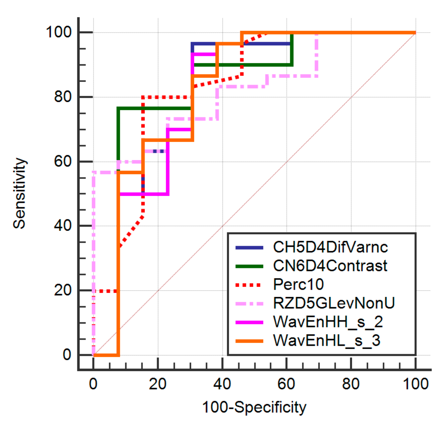
| Texture Parameter | AUC | Sign.lvl. | Youden Index | Cut-Off | Se (%) | Sp (%) |
|---|---|---|---|---|---|---|
| Perc10 | 0.84 (0.7–0.9) | <0.0001 | 0.66 | >21 | 81 (62.3–91.2) | 85.71 (56.2–97.61) |
| WavEnHH_s-2 | 0.81 (0.6–0.91) | 0.0004 | 0.6256 | ≤14.17 | 93.33 (77.9–99.2) | 69.23 (38.6–90.9) |
| CN6D4Contrast | 0.84 (0.65–0.91) | <0.0001 | 0.67 | >22.26 | 77.8 (58.3–91.2) | 93.22 (65.7–98.7) |
| RZD5GLevNonU | 0.82 (0.67–0.92) | <0.0001 | 0.56 | >2447.78 | 56.67 (37.4–74.5) | 100 (75.3–100) |
| CH5D4DifVarnc | 0.82 (0.67–0.92) | 0.0002 | 0.65 | >17.69 | 96.67 (82.8–99.9) | 69.23 (38.6–90.9) |
| CZ2D4DifVarnc | 0.82 (0.67–0.92) | 0.0001 | 0.66 | >21.05 | 96.67 (82.8–99.9) | 69.23 (38.6–90.9) |
| WavEnHL_s-3 | 0.82 (0.67–0.92) | 0.0001 | 0.58 | ≤27.2 | 96.67 (82.8–99.9) | 69.23 (38.6–90.9) |
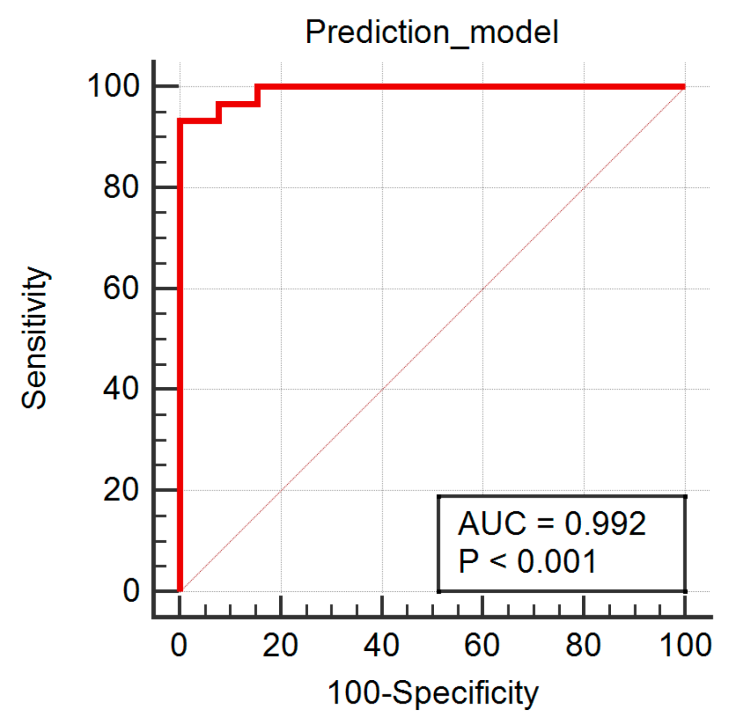
| Independent Variables | Coefficient | Std. Error | p | rpartial | rsemipartial | VIF |
|---|---|---|---|---|---|---|
| CH5D4DifVarnc | 0.05461 | 0.04878 | 0.2705 | 0.1859 | 0.101 | 119.563 |
| CN6D4Contrast | −0.0292 | 0.009469 | 0.004 | −0.4623 | 0.2782 | 7.503 |
| CZ2D4DifVarnc | −0.02923 | 0.04013 | 0.4713 | −0.1222 | 0.06569 | 84.372 |
| Perc10 | 0.0194 | 0.003637 | <0.0001 | 0.6696 | 0.481 | 1.747 |
| RZD5GLevNonU | 0.00008993 | 3.28E-05 | 0.0096 | 0.4203 | 0.2472 | 1.223 |
| WavEnHH_s_2 | −0.01056 | 0.02459 | 0.6702 | −0.07241 | 0.03874 | 12.831 |
| WavEnHL_s_3 | 0.0004019 | 0.01425 | 0.9777 | 0.004767 | 0.002544 | 18.931 |
Publisher’s Note: MDPI stays neutral with regard to jurisdictional claims in published maps and institutional affiliations. |
© 2022 by the authors. Licensee MDPI, Basel, Switzerland. This article is an open access article distributed under the terms and conditions of the Creative Commons Attribution (CC BY) license (https://creativecommons.org/licenses/by/4.0/).
Share and Cite
Mărginean, L.; Ștefan, P.A.; Lebovici, A.; Opincariu, I.; Csutak, C.; Lupean, R.A.; Coroian, P.A.; Suciu, B.A. CT in the Differentiation of Gliomas from Brain Metastases: The Radiomics Analysis of the Peritumoral Zone. Brain Sci. 2022, 12, 109. https://0-doi-org.brum.beds.ac.uk/10.3390/brainsci12010109
Mărginean L, Ștefan PA, Lebovici A, Opincariu I, Csutak C, Lupean RA, Coroian PA, Suciu BA. CT in the Differentiation of Gliomas from Brain Metastases: The Radiomics Analysis of the Peritumoral Zone. Brain Sciences. 2022; 12(1):109. https://0-doi-org.brum.beds.ac.uk/10.3390/brainsci12010109
Chicago/Turabian StyleMărginean, Lucian, Paul Andrei Ștefan, Andrei Lebovici, Iulian Opincariu, Csaba Csutak, Roxana Adelina Lupean, Paul Alexandru Coroian, and Bogdan Andrei Suciu. 2022. "CT in the Differentiation of Gliomas from Brain Metastases: The Radiomics Analysis of the Peritumoral Zone" Brain Sciences 12, no. 1: 109. https://0-doi-org.brum.beds.ac.uk/10.3390/brainsci12010109