
iMIL4PATH: A Semi-Supervised Interpretable Approach for Colorectal Whole-Slide Images

 , , ,
, , , 
Abstract
:Simple Summary
Abstract
1. Introduction
2. Materials and Methods
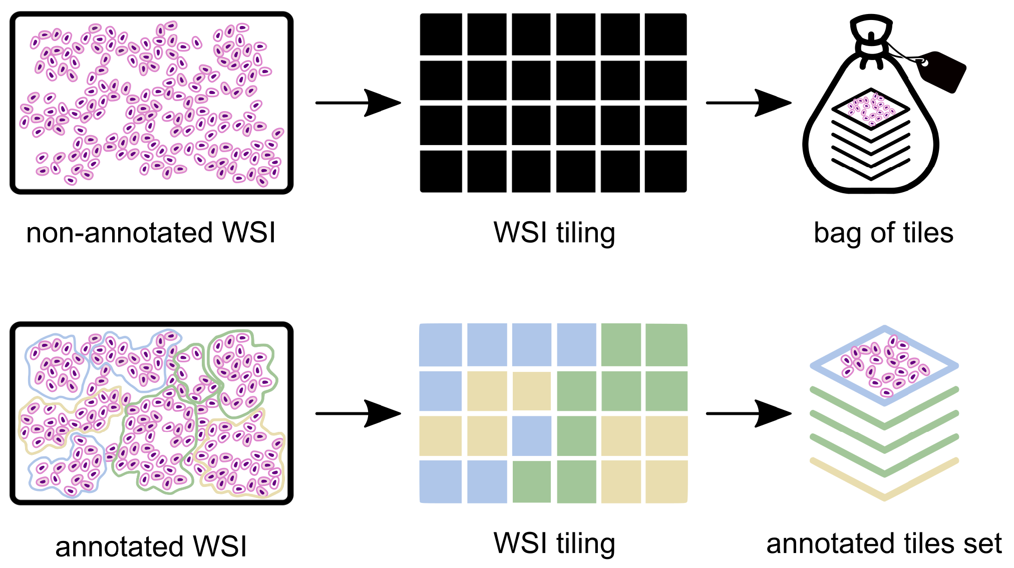
2.1. Data Pre-Processing
2.2. Problem Definition
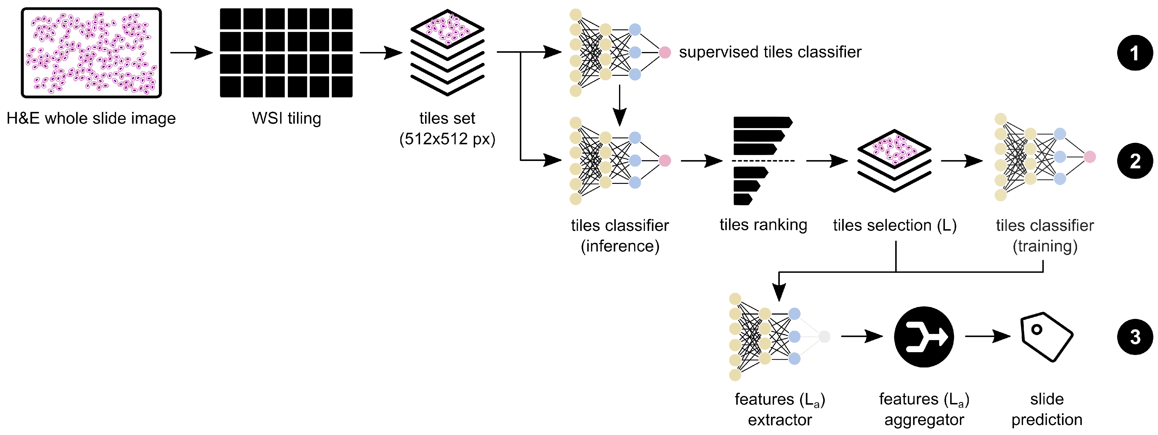
2.3. Model Architecture
2.3.1. Supervised Pre-Training
2.3.2. Weakly Supervised Training
2.3.3. Feature Extraction and Aggregation
- A support-vector machine (SVM) with a radial basis function kernel and a C of 1.0;
- A K-nearest neighbour (KNN) with a K equal to 5;
- A random forest (RF) with a max. depth of 4 and the Gini criterion;
- AdaBoost and XGBoost with 3000 and 5000 estimators, respectively;
- Two distinct multi-layer perceptrons (MLP) with two layers; the first MLP with layers of 75 and 5 nodes—MLP(75;5)—and a second one with layers of 300 and 50 nodes—MLP(300;50).
2.3.4. Interpretability Assessment
2.4. Datasets
2.5. Training Details
3. Results
3.1. Original CRC Dataset Evaluation
3.2. CRC+ Dataset Evaluation
3.3. Domain Generalisation Evaluation
4. Discussion
4.1. Interpretability Assessment
5. Conclusions
Author Contributions
Funding
Data Availability Statement
Acknowledgments
Conflicts of Interest
Abbreviations
| ACC | Accuracy |
| AD | Adenoma |
| Adam | Adaptive moment estimation |
| ADC | Adenocarcinoma |
| AI | Artificial intelligence |
| AUC | Area under the (ROC) curve |
| CNN | Convolutional neural network |
| CRC | Colorectal cancer |
| DL | Deep learning |
| ESGE | European Society of Gastrointestinal Endoscopy |
| GPU | Graphics processing unit |
| H&E | Haemotoxylin and eosin |
| HGD | High-grade dysplasia |
| K-NN | K-nearest neighbour |
| LGD | Low-grade dysplasia |
| MIL | Multiple instance learning |
| MLP | Multilayer perceptron |
| NNeo | Non-neoplastic |
| QWK | Quadratic weighted kappa |
| RF | Random forest |
| RNN | Recurrent neural network |
| ROC | Receiver operating characteristic |
| SVM | Support vector machine |
| WSI | Whole slide image(s) |
References
- International Agency for Research on Cancer (IARC). Global Cancer Observatory. 2021. Available online: https://gco.iarc.fr/ (accessed on 15 March 2022).
- Brody, H. Colorectal cancer. Nature 2015, 521, S1. [Google Scholar] [CrossRef]
- Holmes, D. A disease of growth. Nature 2015, 521, S2–S3. [Google Scholar] [CrossRef] [PubMed]
- Digestive Cancers Europe (DiCE). Colorectal Screening In Europe. Available online: https://bit.ly/3rFxSEL (accessed on 13 March 2022).
- Hassan, C.; Antonelli, G.; Dumonceau, J.M.; Regula, J.; Bretthauer, M.; Chaussade, S.; Dekker, E.; Ferlitsch, M.; Gimeno-Garcia, A.; Jover, R.; et al. Post-polypectomy colonoscopy surveillance: European Society of Gastrointestinal Endoscopy Guideline—Update 2020. Endoscopy 2020, 52, 687–700. [Google Scholar] [CrossRef] [PubMed]
- Mahajan, D.; Downs-Kelly, E.; Liu, X.; Pai, R.; Patil, D.; Rybicki, L.; Bennett, A.; Plesec, T.; Cummings, O.; Rex, D.; et al. Reproducibility of the villous component and high-grade dysplasia in colorectal adenomas <1 cm: Implications for endoscopic surveillance. Am. J. Surg. Pathol. 2013, 37, 427–433. [Google Scholar] [CrossRef] [PubMed]
- Gupta, S.; Lieberman, D.; Anderson, J.C.; Burke, C.A.; Dominitz, J.A.; Kaltenbach, T.; Robertson, D.J.; Shaukat, A.; Syngal, S.; Rex, D.K. Recommendations for Follow-Up After Colonoscopy and Polypectomy: A Consensus Update by the US Multi-Society Task Force on Colorectal Cancer. Gastrointest. Endosc. 2020, 91, 463–485.e5. [Google Scholar] [CrossRef] [PubMed]
- Eloy, C.; Vale, J.; Curado, M.; Polónia, A.; Campelos, S.; Caramelo, A.; Sousa, R.; Sobrinho-Simões, M. Digital Pathology Workflow Implementation at IPATIMUP. Diagnostics 2021, 11, 2111. [Google Scholar] [CrossRef] [PubMed]
- Fraggetta, F.; Caputo, A.; Guglielmino, R.; Pellegrino, M.G.; Runza, G.; L’Imperio, V. A Survival Guide for the Rapid Transition to a Fully Digital Workflow: The “Caltagirone Example”. Diagnostics 2021, 11, 1916. [Google Scholar] [CrossRef]
- Montezuma, D.; Monteiro, A.; Fraga, J.; Ribeiro, L.; Gonçalves, S.; Tavares, A.; Monteiro, J.; Macedo-Pinto, I. Digital Pathology Implementation in Private Practice: Specific Challenges and Opportunities. Diagnostics 2022, 12, 529. [Google Scholar] [CrossRef]
- Madabhushi, A.; Lee, G. Image Analysis and Machine Learning in Digital Pathology: Challenges and Opportunities. Med. Image Anal. 2016, 33, 170–175. [Google Scholar] [CrossRef] [Green Version]
- Rakha, E.A.; Toss, M.; Shiino, S.; Gamble, P.; Jaroensri, R.; Mermel, C.H.; Chen, P.H.C. Current and future applications of artificial intelligence in pathology: A clinical perspective. J. Clin. Pathol. 2020, 74, 409–414. [Google Scholar] [CrossRef]
- Veta, M.; van Diest, P.J.; Willems, S.M.; Wang, H.; Madabhushi, A.; Cruz-Roa, A.; Gonzalez, F.; Larsen, A.B.; Vestergaard, J.S.; Dahl, A.B.; et al. Assessment of algorithms for mitosis detection in breast cancer histopathology images. Med. Image Anal. 2015, 20, 237–248. [Google Scholar] [CrossRef] [PubMed] [Green Version]
- Campanella, G.; Hanna, M.G.; Geneslaw, L.; Miraflor, A.; Werneck Krauss Silva, V.; Busam, K.J.; Brogi, E.; Reuter, V.E.; Klimstra, D.S.; Fuchs, T.J. Clinical-grade computational pathology using weakly supervised deep learning on whole slide images. Nat. Med. 2019, 25, 1301–1309. [Google Scholar] [CrossRef] [PubMed]
- Oliveira, S.P.; Ribeiro Pinto, J.; Gonçalves, T.; Canas-Marques, R.; Cardoso, M.J.; Oliveira, H.P.; Cardoso, J.S. Weakly-Supervised Classification of HER2 Expression in Breast Cancer Haematoxylin and Eosin Stained Slides. Appl. Sci. 2020, 10, 4728. [Google Scholar] [CrossRef]
- Albuquerque, T.; Moreira, A.; Cardoso, J.S. Deep Ordinal Focus Assessment for Whole Slide Images. In Proceedings of the IEEE/CVF International Conference on Computer Vision, Montreal, QC, Canada, 10–17 October 2021; pp. 657–663. [Google Scholar]
- Oliveira, S.P.; Neto, P.C.; Fraga, J.; Montezuma, D.; Monteiro, A.; Monteiro, J.; Ribeiro, L.; Gonçalves, S.; Pinto, I.M.; Cardoso, J.S. CAD systems for colorectal cancer from WSI are still not ready for clinical acceptance. Sci. Rep. 2021, 11, 14358. [Google Scholar] [CrossRef]
- Thakur, N.; Yoon, H.; Chong, Y. Current Trends of Artificial Intelligence for Colorectal Cancer Pathology Image Analysis: A Systematic Review. Cancers 2020, 12, 1884. [Google Scholar] [CrossRef]
- Wang, Y.; He, X.; Nie, H.; Zhou, J.; Cao, P.; Ou, C. Application of artificial intelligence to the diagnosis and therapy of colorectal cancer. Am. J. Cancer Res. 2020, 10, 3575–3598. [Google Scholar]
- Davri, A.; Birbas, E.; Kanavos, T.; Ntritsos, G.; Giannakeas, N.; Tzallas, A.T.; Batistatou, A. Deep Learning on Histopathological Images for Colorectal Cancer Diagnosis: A Systematic Review. Diagnostics 2022, 12, 837. [Google Scholar] [CrossRef]
- Iizuka, O.; Kanavati, F.; Kato, K.; Rambeau, M.; Arihiro, K.; Tsuneki, M. Deep Learning Models for Histopathological Classification of Gastric and Colonic Epithelial Tumours. Sci. Rep. 2020, 10, 1504. [Google Scholar] [CrossRef] [Green Version]
- Tizhoosh, H.; Pantanowitz, L. Artificial intelligence and digital pathology: Challenges and opportunities. J. Pathol. Inform. 2018, 9, 38. [Google Scholar] [CrossRef]
- Wei, J.W.; Suriawinata, A.A.; Vaickus, L.J.; Ren, B.; Liu, X.; Lisovsky, M.; Tomita, N.; Abdollahi, B.; Kim, A.S.; Snover, D.C.; et al. Evaluation of a Deep Neural Network for Automated Classification of Colorectal Polyps on Histopathologic Slides. JAMA Netw. Open 2020, 3, e203398. [Google Scholar] [CrossRef] [Green Version]
- Song, Z.; Yu, C.; Zou, S.; Wang, W.; Huang, Y.; Ding, X.; Liu, J.; Shao, L.; Yuan, J.; Gou, X.; et al. Automatic deep learning-based colorectal adenoma detection system and its similarities with pathologists. BMJ Open 2020, 10, e036423. [Google Scholar] [CrossRef] [PubMed]
- Xu, L.; Walker, B.; Liang, P.I.; Tong, Y.; Xu, C.; Su, Y.; Karsan, A. Colorectal cancer detection based on deep learning. J. Pathol. Inf. 2020, 11, 28. [Google Scholar] [CrossRef] [PubMed]
- Wang, K.S.; Yu, G.; Xu, C.; Meng, X.H.; Zhou, J.; Zheng, C.; Deng, Z.; Shang, L.; Liu, R.; Su, S.; et al. Accurate diagnosis of colorectal cancer based on histopathology images using artificial intelligence. BMC Med. 2021, 19, 1–12. [Google Scholar] [CrossRef] [PubMed]
- Yu, G.; Sun, K.; Xu, C.; Shi, X.H.; Wu, C.; Xie, T.; Meng, R.Q.; Meng, X.H.; Wang, K.S.; Xiao, H.M.; et al. Accurate recognition of colorectal cancer with semi-supervised deep learning on pathological images. Nat. Commun. 2021, 12, 1–13. [Google Scholar] [CrossRef] [PubMed]
- Marini, N.; Otálora, S.; Ciompi, F.; Silvello, G.; Marchesin, S.; Vatrano, S.; Buttafuoco, G.; Atzori, M.; Müller, H. Multi-Scale Task Multiple Instance Learning for the Classification of Digital Pathology Images with Global Annotations. In Proceedings of the MICCAI Workshop on Computational Pathology, Strasbourg, France, 27 September–1 October 2021; Volume 156, pp. 170–181. [Google Scholar]
- Ho, C.; Zhao, Z.; Chen, X.F.; Sauer, J.; Saraf, S.A.; Jialdasani, R.; Taghipour, K.; Sathe, A.; Khor, L.Y.; Lim, K.H.; et al. A promising deep learning-assistive algorithm for histopathological screening of colorectal cancer. Sci. Rep. 2022, 12, 1–9. [Google Scholar] [CrossRef]
- Kirk, S.; Lee, Y.; Sadow, C.A.; Levine, S.; Roche, C.; Bonaccio, E.; Filiippini, J. Radiology Data from The Cancer Genome Atlas Colon Adenocarcinoma [TCGA-COAD] collection. Cancer Imaging Arch. 2016. [Google Scholar] [CrossRef]
- Kirk, S.; Lee, Y.; Sadow, C.A.; Levine, S. Radiology Data from The Cancer Genome Atlas Rectum Adenocarcinoma [TCGA-READ] collection. Cancer Imaging Arch. 2016. [Google Scholar] [CrossRef]
- Clark, K.; Vendt, B.; Smith, K.; Freymann, J.; Kirby, J.; Koppel, P.; Moore, S.; Phillips, S.; Maffitt, D.; Pringle, M.; et al. The Cancer Imaging Archive (TCIA): Maintaining and Operating a Public Information Repository. J. Digit. Imaging 2013, 26, 1045–1057. [Google Scholar] [CrossRef] [Green Version]
- Platform, P.A. PAIP. 2020. Available online: http://www.wisepaip.org (accessed on 20 April 2022).
- Otsu, N. A Threshold Selection Method from Gray-Level Histograms. IEEE Trans. Syst. Man Cybern. 1979, 9, 62–66. [Google Scholar] [CrossRef] [Green Version]
- He, K.; Zhang, X.; Ren, S.; Sun, J. Deep residual learning for image recognition. In Proceedings of the IEEE Conference on Computer Vision and Pattern Recognition, Las Vegas, NV, USA, 27–30 June 2016; pp. 770–778. [Google Scholar] [CrossRef] [Green Version]
- Guo, C.; Pleiss, G.; Sun, Y.; Weinberger, K.Q. On calibration of modern neural networks. In Proceedings of the International Conference on Machine Learning, Sydney, Australia, 6–11 August 2017; pp. 1321–1330. [Google Scholar]
- Pathcore. Sedeen Viewer. 2020. Available online: https://pathcore.com/sedeen (accessed on 18 April 2021).
- Montezuma, D.; Fraga, J.; Oliveira, S.; Neto, P.; Monteiro, A.; Pinto, I.M. Annotation in digital pathology: How to get started? Our experience in classification tasks in pathology. In Proceedings of the 33rd European Congress of Pathology, Online, 29–31 August 2021; Volume 479, p. S320. [Google Scholar]


| NNeo | LG | HG | Total | ||
|---|---|---|---|---|---|
| # slides | 300 (6) | 552 (35) | 281 (59) | 1133 (100) | |
| CRC dataset [17] | # annotated tiles | 49,640 | 77,946 | 83,649 | 211,235 |
| # non-annotated tiles | - | - | - | 1,111,361 | |
| # slides | 663 (12) | 2394 (207) | 1376 (181) | 4433 (400) | |
| CRC+ dataset | # annotated tiles | 145,898 | 196,116 | 163,603 | 505,617 |
| # non-annotated tiles | - | - | - | 5,265,362 |
| Method | Annotated Samples | Training Tiles | Aggregation Tiles | QWK | ACC | Sensitivity | Specificity |
|---|---|---|---|---|---|---|---|
| Oliveira et al. | 0 | 1 | 1 | 0.795 | 84.17% | 0.933 | - |
| Oliveira et al. | 100 | 1 | 1 | 0.863 | 88.42% | 0.957 | - |
| Supervised baseline | 100 | - | 1 | 0.027 | 29.73% | 0.449 | 0.796 |
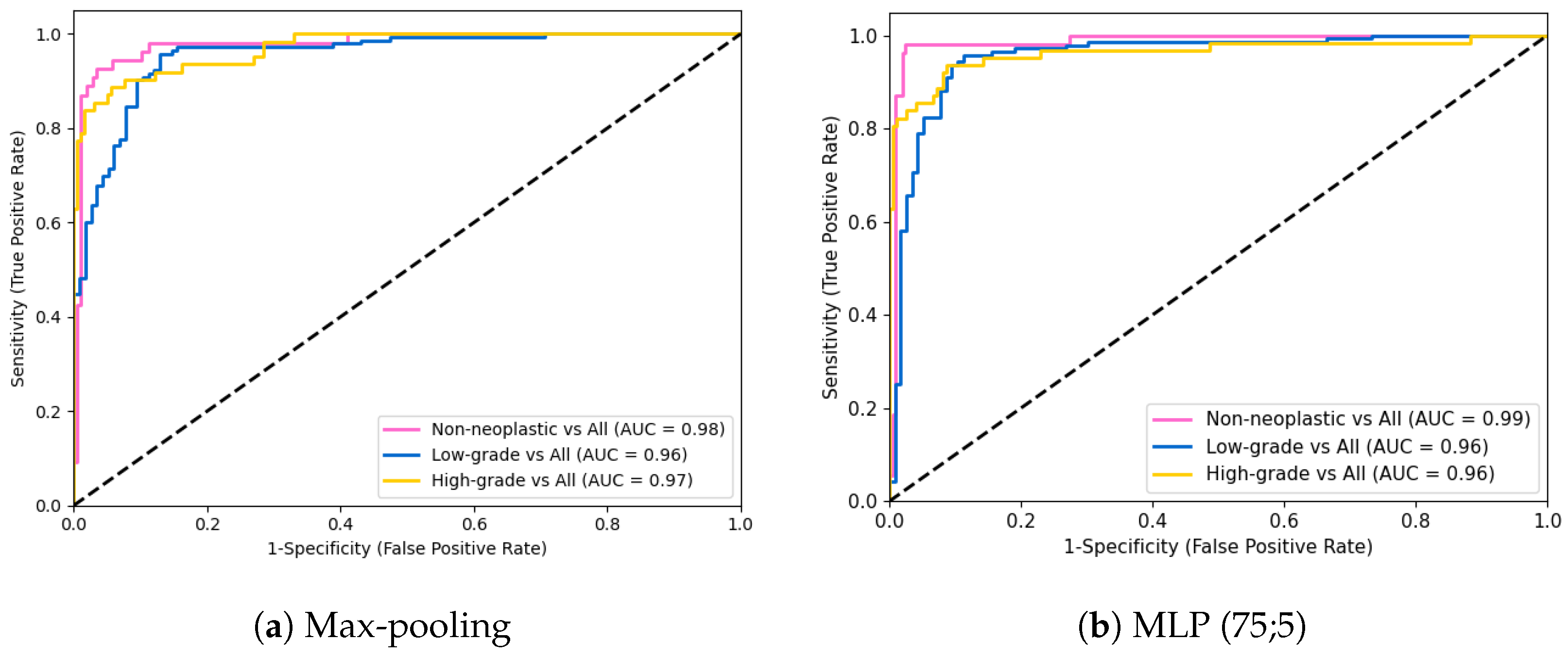
| Max-pooling | 100 | 5 | 1 | 0.881 | 91.12% | 0.990 | 0.852 |
| MLP (75;5) | 100 | 5 | 7 | 0.906 | 91.89% | 0.980 | 0.981 |
| SVM | 0.887 | 90.35% | 0.971 | 0.944 | |||
| KNN | 0.890 | 90.35% | 0.971 | 0.981 | |||
| RF | 0.878 | 89.57% | 0.966 | 0.963 | |||
| AdaBoost | 0.862 | 88.03% | 0.961 | 0.907 | |||
| XGBoost | 0.879 | 89.58% | 0.961 | 0.963 | |||
| SVM + KNN | 100 | 5 | 7 | 0.898 | 91.12% | 0.971 | 0.981 |
| SVM + RF + KNN | 100 | 5 | 7 | 0.893 | 90.73% | 0.971 | 0.981 |
| Predicted | ||||
|---|---|---|---|---|
| Actual | NNeo | LG | HG | |
| NNeo | 53 | 1 | 0 | |
| LG | 4 | 137 | 2 | |
| HG | 0 | 14 | 48 | |
| Method | Training Samples | Test Samples | Aggregation Tiles | QWK Score | ACC | Sensitivity | Specificity |
|---|---|---|---|---|---|---|---|
| Max-pooling | 874 (100) | 259 | 1 | 0.881 | 91.12% | 0.990 | 0.852 |
| MLP (75;5) | 7 | 0.906 | 91.89% | 0.980 | 0.981 | ||
| MLP (300;50) | 7 | 0.885 | 91.12% | 0.966 | 0.981 | ||
| Max-pooling | 1174 (400) | 259 | 1 | 0.874 | 91.12% | 0.985 | 0.907 |
| MLP (75;5) | 7 | 0.838 | 86.49% | 0.946 | 0.926 | ||
| MLP (300;50) | 7 | 0.850 | 87.26% | 0.941 | 0.944 | ||
| Max-pooling | 4174 (400) | 259 | 1 | 0.834 | 89.96% | 0.980 | 0.870 |
| MLP (75;5) | 7 | 0.810 | 83.78% | 0.922 | 0.889 | ||
| MLP (300;50) | 7 | 0.816 | 83.01% | 0.927 | 0.926 | ||
| Max-pooling | 3424 (400) | 1009 | 1 | 0.884 | 89.89% | 0.992 | 0.815 |
| MLP (75;5) | 7 | 0.871 | 88.89% | 0.982 | 0.839 | ||
| MLP (300;50) | 7 | 0.888 | 90.19% | 0.988 | 0.857 |
| Method | ACC | Binary ACC | Sensitivity |
|---|---|---|---|
| Max-pooling | 71.55% | 80.60% | 0.805 |
| MLP (75;5) | 61.20% | 75.43% | 0.753 |
| MLP (300;50) | 58.62% | 74.13% | 0.740 |
| Method | ACC | Binary ACC | Sensitivity |
|---|---|---|---|
| Max-pooling | 99.00% | 100.00% | 1.000 |
| MLP (75;5) | 77.00% | 98.00% | 0.980 |
| MLP (300;50) | 77.00% | 98.00% | 0.980 |
Publisher’s Note: MDPI stays neutral with regard to jurisdictional claims in published maps and institutional affiliations. |
© 2022 by the authors. Licensee MDPI, Basel, Switzerland. This article is an open access article distributed under the terms and conditions of the Creative Commons Attribution (CC BY) license (https://creativecommons.org/licenses/by/4.0/).
Share and Cite
Neto, P.C.; Oliveira, S.P.; Montezuma, D.; Fraga, J.; Monteiro, A.; Ribeiro, L.; Gonçalves, S.; Pinto, I.M.; Cardoso, J.S. iMIL4PATH: A Semi-Supervised Interpretable Approach for Colorectal Whole-Slide Images. Cancers 2022, 14, 2489. https://0-doi-org.brum.beds.ac.uk/10.3390/cancers14102489
Neto PC, Oliveira SP, Montezuma D, Fraga J, Monteiro A, Ribeiro L, Gonçalves S, Pinto IM, Cardoso JS. iMIL4PATH: A Semi-Supervised Interpretable Approach for Colorectal Whole-Slide Images. Cancers. 2022; 14(10):2489. https://0-doi-org.brum.beds.ac.uk/10.3390/cancers14102489
Chicago/Turabian StyleNeto, Pedro C., Sara P. Oliveira, Diana Montezuma, João Fraga, Ana Monteiro, Liliana Ribeiro, Sofia Gonçalves, Isabel M. Pinto, and Jaime S. Cardoso. 2022. "iMIL4PATH: A Semi-Supervised Interpretable Approach for Colorectal Whole-Slide Images" Cancers 14, no. 10: 2489. https://0-doi-org.brum.beds.ac.uk/10.3390/cancers14102489