
Hyperspectral Imaging to Characterize Table Grapes


1
USC 1422 GRAPPE, INRAE, Ecole Supérieure d’Agricultures, SFR 4207 QUASAV, 55 Rue Rabelais, BP 30748, 49007 Angers CEDEX 01, France
2
Dipartimento di Scienze e Tecnologie Alimentari per una filiera agro-alimentare Sostenibile, Università Cattolica del Sacro Cuore, Via Emilia Parmense 84, 29122 Piacenza, Italy
*
Author to whom correspondence should be addressed.
Chemosensors 2021, 9(4), 71; https://0-doi-org.brum.beds.ac.uk/10.3390/chemosensors9040071
Submission received: 28 January 2021
/
Revised: 24 March 2021
/
Accepted: 29 March 2021
/
Published: 1 April 2021
(This article belongs to the Section Analytical Methods, Instrumentation and Miniaturization)
Abstract
:Table grape quality is of importance for consumers and thus for producers. Its objective quality is usually determined by destructive methods mainly based on sugar content. This study proposed to evaluate the possibility of hyperspectral imaging to characterize table grapes quality through its sugar (TSS), total flavonoid (TF), and total anthocyanin (TA) contents. Different data pre-treatments (WD, SNV, and 1st and 2nd derivative) and different methods were tested to get the best prediction models: PLS with full spectra and then Multiple Linear Regression (MLR) were realized after selecting the optimal wavelengths thanks to the regression coefficients (β-coefficients) and the Variable Importance in Projection (VIP) scores. All models were good at showing that hyperspectral imaging is a relevant method to predict sugar, total flavonoid, and total anthocyanin contents. The best predictions were obtained from optimal wavelength selection based on β-coefficients for TSS and from VIPs optimal wavelength windows using SNV pre-treatment for total flavonoid and total anthocyanin content. Thus, good prediction models were proposed in order to characterize grapes while reducing the data sets and limit the data storage to enable an industrial use.
Keywords:
hyperspectral imaging; phenolics; anthocyanin; table grapes; total soluble solids; PLS; MLR; prediction; model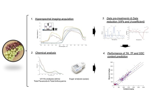
1. Introduction
Grapes are one of the most consumed fruits in the word, as fresh fruit, grape juice, raisins, and wine. About 36% of grape production concerned the fresh fruit consumption (International Organization of Vine and Wine statistics). The European production of table grapes (~1.9 million tons) is mainly located in the Mediterranean area, with the domination of Italy (61%), Greece (16%), Spain (15%), and France (1.5%) [1]. The French production of table grapes is mostly in Vaucluse and Tarn-et-Garonne. About 80% of the production concern only three varieties: Alphonse Lavallée, Chasselas, and Muscat de Hambourg. French table grape production (~30,000 tons) represents approximately 40% of the national consumption, while the 60% remaining is mainly imported from Spain and Italy.
The right commercial harvest of table grapes is usually determined by different parameters like skin color, texture softening, titratable acidity, total soluble solids, and sometimes with flavonoid content, and aromatic compounds [2,3]. Visual attributes of table grapes, such as intensity and uniformity of color, large size of berries, and brightness are the main characteristics that influence consumer choice [4,5]. Color is of high importance to assess quality in the food industry [6]. Furthermore, some studies have found clear evidences that a greater consumption of fresh grapes decreases the risk of cardiovascular diseases and cancer [7,8]. This beneficial effect is mainly related to the presence of minerals, fibers, vitamins, and phytochemical compounds including flavonoids and anthocyanins [9,10]. However, the concentration of these quality attributes changes during postharvest storage and thus influence sensory perception and nutritional value of table grapes.
The quality parameters of table grapes can be assessed by a few methods [11,12,13]. Nevertheless, conventional analytical methods need a preparation of the sample, they are destructive and limit thus their use in an on-line/in-line industry for quality monitoring [14,15,16]. These methods require furthermore time and solvents and generate chemical waste. Despite being time consuming and expensive, the destructive analytical approach provides data for a limited number of samples, and, thus, their statistical relevance could be limited [17]. Several studies in the field of post-harvest are focused on non-destructive analytical techniques, which are fast, reliable, and allow to analyze a higher number of samples and repetitions of the same batch in real time.
The development of non-destructive techniques suitable to increase the number of samples analyzed is the objective of current researches, in any field. The possibility to get real-time information of quality attributes of fruits and a robust statistical data analysis is clearly aimed at these studies [18]. Infrared spectroscopy (FT-NIR and ATR-FTIR) has been applied for the prediction of procyanidin concentration [19], total polyphenol content [20], malvidin-3-O-glucoside, pigmented polymers and tannin contents [21] in cocoa, green tea, and fermenting red wine, respectively. This technology has also been employed to determine, pH, total soluble solids, glycerol, and gluconic acid in grape juice [22] and to measure condensed tannins and the dry matter in homogenized red grape berries [23].
Hyperspectral imaging spectroscopy (HIS) is a non-destructive spectroscopic technique that records hundreds of narrow-wavelength bands and spatial positions [24]. This technique is a system combining imaging and spectroscopy [25,26], providing the spatial information of spectra obtained from each pixel in the hyperspectral image [25,27]. A hyperspectral image is thus a three-dimensional (3D) cube that includes spatial information in two dimensions (of x rows and y columns) and spectral information in one dimension (of λ wavelengths) [28]. The hyperspectral image cube “hypercube” consists of a series of sub-images at small interval wavelengths ranging from 400 to 2500 nm in VIS and NIR spectral regions.
Over the last decade, HIS has been applied for fruit and vegetable quality assessment [24,27], food safety control [29,30,31], and classification tool [32,33]. Likewise, total acidity, pH, soluble solid content, technological maturity, total anthocyanin concentration, antioxidant activity, and total phenolic compounds in grapes were determined using VIS−NIR hyperspectral imaging of few fruits [34,35] but a lack of study appeared for table grapes. HIS has an advantage compared to the spectroscopic method, i.e., it acquires the spectral information on a larger area of the fruit surface analyzed and therefore considers the heterogeneity within the berries, on the contrary to a spectrophotometer [35,36]. Moreover, the conventional RGB imaging detects only surface features and could not be able to measure the chemical composition of the fruit. The HSI technique, instead, acquires information in a different region of the electromagnetic spectrum, which is strictly linked to the chemical composition of the samples [37]. The HIS has also the advantage of receiving spatially distributed spectral responses at each pixel of a fruit image. Another advantage is that once appropriate calibration models are developed, they can be re-inserted in the hypercube to create chemical mapping images. For the grape industry, the interest would be to separate berries one by one depending on their average representative spectrum, and not spatial information within each berry, in order to get several final batches for different transformations, storage conditions, or quality arrays.
The objective of this study was to determine if hyperspectral imaging would be able to predict the sugar content and the concentration of Total Flavonoids and Total Anthocyanins of white and red table grapes. Additionally, as keeping whole spectra for all samples would generate big data to manage and a higher time to analyze in a potential on-line tool, the second objective was to define if it was possible to reduce the number of wavelengths with still having good models of prediction. Thus, this study developed calibration and prediction models for three quality attributes of table grape based on hyperspectral imaging:
- I.
- Developing partial least square (PLS) models to validate the correlation between hyperspectral imaging spectra and Total Anthocyanins (TA) and Total Flavonoid (TF) contents and Total Soluble Solids (TSS), using the visible and short-wave near-infrared region;
- II.
- Selecting the lowest number of optimal wavelengths, based on regression coefficient (RC) and Variable Importance in Projection (VIPs) algorithms, which gave the highest correlation between the spectral data and the three selected quality parameters;
- III.
- Developing Multiple Regression Models (MLR) using spectra from only the optimal wavelengths and then checking the validation of the developed calibration models.
The novelty of this study was to estimate the potential of hyperspectral imaging as possible prediction model supplier for quality parameters (TF, TA, and TSS) usable for all table grapes. Moreover, the use of specific wavelengths and not the full spectra for these products represented a new approach.
2. Materials and Methods
2.1. Chemicals
The following chemicals were used: ethanol 96%, hydrochloric acid ≥ 37%, (FlukaTM, Muskegon, MI, USA), malvidin-3-O-glucoside 92.7% (Extrasynthese, Genay, France), and (+)-catechin 99.2% (Sigma–Aldrich, Saint-Louis, MI, USA). All the chemicals were at least of analytical grade. Ultrapure water was prepared from deionized water obtained a Milli-Q system (Millipore SAS, Molsheim, France).
2.2. Samples
Seven table grapes varieties were bought in regional markets at commercial harvest ripeness: Three white table grapes (Sugarone Superior Seedless, Thompson Seedless, and Victoria) and four red/black table grapes (Sable Seedless, Alphonse Lavallée, Lival, and Black Magic). Alphonse Lavallée and Lival were chosen because they represented French cultivars produced in the south-east of France and mostly consumed throughout the country. The other 5 cultivars were chosen because they are largely diffused around the world. Approximately 5 kg of clusters randomly selected were sampled for each cultivar. A subsample of 50 berries of each variety, with short attached pedicels, was collected from different bunch parts (shoulders, middle, and bottom). Grapes were then washed and gently dried with absorbent paper, stored at 4 °C until the HIS acquisitions.
For the 7 varieties, 50 berries of each were analyzed in triplicate by hyperspectral imaging, then they were chemically analyzed, leading to 350 mean spectra and 350 TF and TSS and 200 TA. Then, PLS and MLR were applied on pre-treated data.
2.3. Hyperspectral Imaging System (HIS)
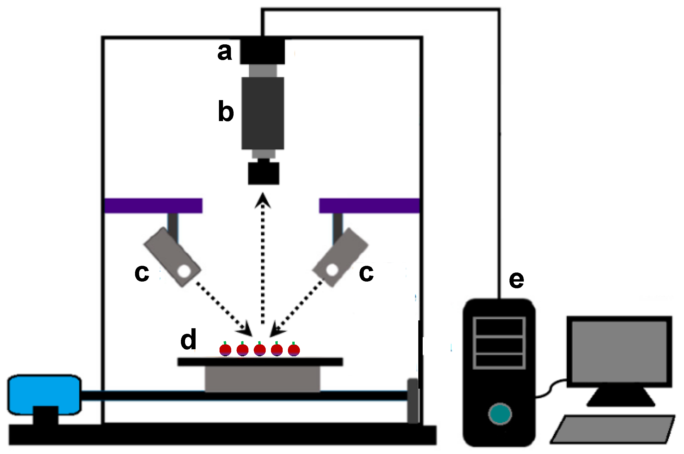
The system is composed of the following components (Figure 1): (a) a hyperspectral imaging camera (Pika L, Resonon, Bozeman, MT, USA) coupled with an objective lenses (Xenoplan 1.4/23, Schneider-Kreuznach, Bad Kreuznach, Germany); (b) an illumination unit, which consists of four 35 W quartz tungsten halogen (QTH) MR16 35 W lamps adjusted at angle of 45° to illuminate the camera’s field of view; (c) a mounting tower; and (d) a transport stage (PS-12-20-1.0, Servo Systems Co., Rockaway, NJ, USA), with motor (DMX-J-SA-17, Arcus Technology Inc., Livermore, CA, USA). The sensor has 900 spatial channels each with 281 spectral channels covering the range from 387 to 1026 nm. The maximum spectral resolution is 2.1 nm. The camera was set up at 450 mm from the target. The spectral images were collected in a dark room where only the halogen light source was used. The HIS was controlled by a PC with the software SpectrononPRO (Resonon, Bozeman, MT, USA) for image acquisition.
2.4. Image Acquisition
The samples were kept at room temperature (20 °C) for 1 h prior to the imaging acquisition in the reflectance mode. The hyperspectral image of each sample (one berry) was recorded in three different berry positions corresponding to berry rotations of approximately 120° between positions. The berries reflectance measurement was made along the berry “equator” when considering the pedicel to be the “pole.” This is a common practice reported by several articles [38,39]. The hyperspectral images were recorded by the SpectrononPRO software (Resonon, Bozeman, MT, USA) using an exposure time of 12 ms and a stage speed of 11 mm s−1 with a gain of 10. The spectral data in the wavelength range of 411–1000 nm was used in the data analysis for removing noise and reducing data redundancy out of this range. For each sample (50 berries), three reflectance spectra were collected, corresponding to the berry rotations, and averaged over the spatial dimension.
2.5. Preprocessing of Hyperspectral Images
All the acquired images were processed and analyzed using SpectrononPro 5.1 Hyperspectral Imaging System software (Resonon, Bozeman, MT, USA). The hyperspectral images were firstly corrected with a white and a dark reference (WD). The dark reference was used to remove the effect of dark current of the CCD detectors, which are thermally sensitive.
The corrected reflectance (R) is estimated using the following Equation (1):
where S is the intensity of an image, W is the intensity of the white reference image (Teflon white board with 99% reflectance), and D is the intensity of the dark reference image (with 0% reflectance) recorded by turning off the lighting source with the lens of the camera completely covered. The corrected reflectances were the basis for the subsequent image analysis to extract the spectral response of each fruit, select effective wavelengths, and predict physicochemical parameters.
2.6. Data Analysis
2.6.1. Determination of Reference Parameters: Total Soluble Solids (TSS), Total Anthocyanin (TA), and Total Flavonoid Content (TF)
Immediately after image acquisition, each berry was subjected to the determination of Total Soluble Solids (TSS), Total Flavonoids (TF), and Total Anthocyanins (TA). Each berry was weighed, manually peeled, and the juice was collected separately. Total Soluble Solids were measured by a portable refractometer (Mettler Toledo Refracto 30PX) with a 0.2°Brix incertitude. The skins were separately weighed and extracted four times with 7.5 mL of hydrochloride ethanol solution (ethanol/water/hydrochloric acid 70/30/1 v/v/v). The samples were shaken for 60′ with a horizontal shaker VXR vibrax (IKA-Werke, Staufen, Germany) at 1500 rpm and centrifuged at 5000 rpm for 5′, and the supernatant was collected in a volumetric flask. The supernatants were collected together, brought to the volume of 25 mL and, stored at −80 °C until analyses. The quantification of TA and TF was carried out spectrophotometrically by recording the UV–visible spectra in the range of 220–700 nm using a Safas UV mc2 spectrophotometer (Safas, Monaco City, Monaco) and measuring the absorption values at 280 and 520 nm, as previously reported [40]. The results were expressed as mg (+)-catechin equivalents/kg fresh grape and mg malvidin-3-O-glucoside equivalents/kg fresh grape for the flavonoids and anthocyanins, respectively.
2.6.2. Spectral Analysis for Predicting Quality Attributes
- Collecting spectral data
Only regions of interest (ROIs) were collected as already described [41] and an average spectrum was calculated by averaging the relative reflectance spectra.
- Spectra pre-treatments
To overcome or reduce unwanted spectral variation, baseline shifts, and various noise, a series of pre-treatment methods was applied on the mean spectral data to decrease the influence of high-frequency random noises, the nonuniformity in samples, and the surface scattering. Before building the validation model, different Equations (2) to (4) were used for spectral pre-treatments [42]:
SNV: Standard Normal Variate (SNV). The average intensity (Amean) and standard deviation (ASD) of the spectrum are calculated and inserted in Equation (2):
1st derivative: The first derivatives was calculated using the symmetric difference quotient 1st derivative (3):
2nd derivative: The second derivate was calculated using the symmetric difference quotient 2nd derivate (4):
With i = 1 to N, N being the number of samples.
2.6.3. Hyperspectral Imaging Calibration
- Model establishment
The use of chemometrics in modeling spectral data is widely employed, being considered as a standard procedure for building predictive models in the analysis of hyperspectral images. The partial least squares (PLS) analysis between one quality attribute (TA and TF or TSS) and the spectral data (average spectra with 276 wavelengths in the range from 411 to 1000 nm) was conducted using XLSTAT software (Addinsoft, Paris, France, 2019). No outlier detection was performed in order to keep all spectra and the heterogeneity due to the vegetal material.
A total of 350 reflectance mean spectra were obtained from 350 berries. The calibration and validation sets were established by ordering the fruit samples according to their physicochemical references. Briefly, 4 samples per varieties, i.e., 28 samples in total were randomly selected for the prediction set. The two highest and two lowest values were assigned to the calibration set. Afterward, two-thirds of the samples were randomly selected as calibration data and one-third of the samples were defined as validation data in a 2:1 leave-one-out procedure. Thus, calibration set and validation set were independent.
PLS regression used to develop calibration models was carried out with two calibration sample sets: (i) N = 207 samples for TF and TSS and (ii) N = 116 samples for TA. The building of PLS models for TF and TSS took into account both the white and red table grape cultivars, while for TA was considered only the red and rosé grape cultivars since white grapes do not have anthocyanins. To reduce the probability of an over fitting of the experimental data [43], PLS models with 1–15 latent variables (LVs) were fitted, and the model with a number of PLS factors that maximized the coefficient of determination (R2cal) for the calibration and minimized the root mean square error of calibration (RMSEC) was selected. These two parameters would allow the evaluation of the models.
- Hyperspectral imaging model validation
Two validation sets (N = 103 samples for TF and TSS; N = 56 samples for TA) were used to calculate the root mean square error of validation (RMSEV), the coefficient of determination (R2val), the Bias, and the Ratio Performance Deviation (RPD) of the PLS models as follow [42]:
where N is the number of samples, R is the number of PLS factors, is the reference value for sample i, and is the predicted value for sample i.
- Hyperspectral imaging prediction
The quality of prediction of the models was tested using 4 samples per variety. The level of prediction is discussed base on R2pr and RMSEP values. The RMSEP was calculated as follow:
- Selection of optimal wavelengths
Spectral wavelengths in hyperspectral images are characterized by their large degree of dimensionality with collinearity and redundancy. Researchers are often interested in finding the most important wavelengths which contribute to the evaluation of quality parameters and eliminate wavelengths having no discrimination power. After proving the good performance of the PLS models on the validation set, the next step was to select only the wavelengths that showed the maximum spectral information.
The regression coefficients (RC), also called β-coefficients, and the Variable Importance in Projection (VIP) scores were applied to select the most informative wavelengths, which provided the best PLS calibration model built with the full spectrum as variables. The wavelengths that corresponded to the highest absolute values of β-coefficients were considered optimal wavelengths [44]. Based on the studies conducted by Olah et al. [45], all wavelengths at which the VIP scores were above a threshold of 1.0 (highly influential) were selected and compared with those identified using β-coefficients. In this study, only the wavelengths with highest β-coefficients (absolute values) from one side and highest VIP scores (above the threshold of 1.0) on another side were selected to establish Multiple Linear Regression (MLR) models, instead of using the whole spectral range. Moreover, all the wavelengths with VIP score above 1 (spectral windows) were also used to carry out another PLS regression model in order to improve its performance.
2.6.4. Statistical Analyses
One way ANOVA on quality attributes of table grapes was performed with XLSTAT 2019.1 software (Addinsoft, Paris, France). Mean values were separated with Tukey’s test (p < 0.05) to present the significant differences between varieties.
3. Results
3.1. Grape Composition
Berries from each grape variety were characterized by their sugar content (Total Soluble Solids (TSS)), their Total Flavonoid content (TF), and Total Anthocyanin content (TA). Table 1 shows that the selected varieties had different total flavonoid content, from 201 mg kg−1 FW for Victoria grapes to 1642 mg kg−1 FW for Lival grapes, with white grapes presenting the lowest phenolic concentration as expected. This result is in agreement with Mikulic-Petkousek et al. [46], which showed that Victoria variety has a low phenolic content. Similarly, a large amount of total anthocyanin content was observed from 217 mg kg−1 FW for Alphonse Lavallée to 590 mg kg−1 FW for Sable seedless. Their sugar concentration was between 14.0 g/100 g (Victoria) to 24.8 g/100 g (Alphonse Lavallée) corresponding to ripening level [2]. Statistics showed that TF, TA, and TSS were significantly dependent on the grape cultivar.
3.2. Spectral Profiles
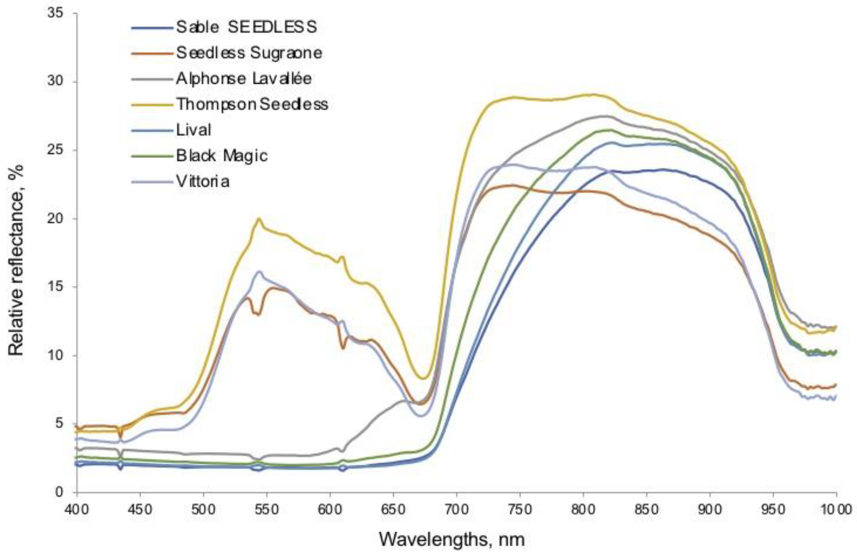
The mean reflectance spectra profile of each grape variety is presented in Figure 2. These spectra obtained by HIS showed clear differences between the grape varieties, as already reported by Baiano et al. [47] on 7 other varieties. White grapes exhibited important reflectance from about 500–650 nm on the contrary of reds. Chlorophyll pigments absorb indeed around 540 nm giving the green-yellow color to these varieties as hypothesized by Costa et al. (2019) [48]. All grapes presented much higher reflectance percentage between 700 and 950 nm, with a mix of intensity between reds and whites but varieties showed similar trends depending on the variety color: whites had higher intensity around 700–720 nm, which decreased to 950 nm, and reds showed flattened bell curve with a maximum around 820 nm. Absorption band at 840 nm is mainly due to sugar [47] and more than 960 nm due to water [48,49].
3.3. Modelization of Table Grape Composition Using the Whole Spectral Range of 411–1000 nm
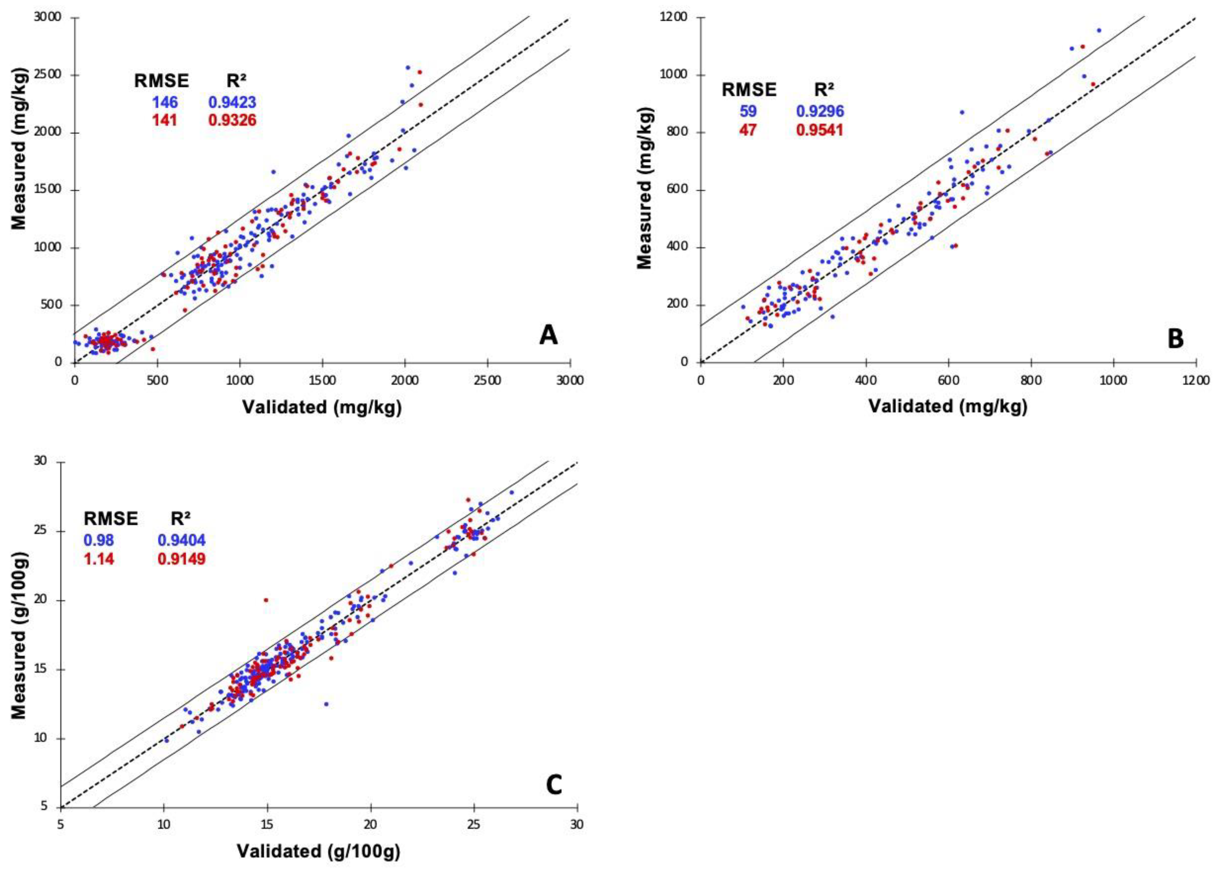
PLS were developed to establish the relationship between the spectral data and the corresponding TA, TF, and TSS content analyzed by conventional chemical method. First of all, the whole dataset was dedicated to select the best pre-treatment for each quality parameter. The results are reported in Table 2. Five parameters were used to select the best model: R², LVs, RMSE, and Bias. RMSE has to be minimized and RPD has to be maximized [48]. HIS data were relevant [49] for modelizing Total Flavonoid, Total Anthocyanin contents, and TSS, since all determination coefficients (R2cal and R2val) were over 0.87 (Table 2). All pretreatments showed good results. Thus, we decided for similar range of R² and RMSE, to select the pre-treatment leading to the lower number of LVs, that is to say the SNV pre-treatment for all quality parameters. In details, for the modelization of TF, the SNV pre-treatment used only 9 LVs, with R2cal = 0.94, R2val = 0.93, with RMSEV = 141 mg kg−1. For Total Anthocyanins, the SNV model was characterized by R2cal = 0.93, R2val = 0.95, and RMSEV = 47 mg/kg with only 3 LVs. Finally, for TSS, the model, thanks to 10 latent variables, generated a R2cal = 0.94 and a R2val = 0.91 with RMSEV = 1.1 g/100 g. As for residual validation deviation (RPD), selected pre-treatments (mainly WD) generated values close to 4, which suggest the capability of the models to provide a good quantification and satisfactory prediction of TF, TA, and TSS [50,51]. The relatively low number of LVs of the models generated, and in particular for TA, and the fact that the models were built using grape berries of seven different cultivar contributed to the robustness of the models. Moreover, measured data vs. validated data were plotted for the three models selected (Figure 3). These graphs validated the selected models proving the ability of hyperspectral imaging data to predict TF, TA, and TSS in table grapes.
It is interesting to note that for TF and TSS a bimodal effect could be observed. That phenomenon is due to the white varieties in the case of TF, since they had the lowest TF values (as expected) compared to the other varieties. Nevertheless, the prediction of low values of TF could be considered uncertain since the concentration of TF below 500 mg/kg seemed not to follow a linear trend even if they positively contribute to the model (data not shown). For TSS, that effect was due to the rosé grapes since they presented the highest TSS values.
The predictions of these quality parameters were good since the determination coefficients obtained ranged between 0.92 and 0.98 for the pre-treatments selected above. The RMSEP was in the same order of magnitude than those of the validation and calibration sets, and even a bit better, i.e., the RMSEP were of 33 mg/kg for TA and of 0.9 for TSS, whereas the RMSEV were of 47 mg/kg for TA and 1.1 for TSS. This result shows that the method used for the validation was good. Thus, these results showed also that all grape varieties could be gathered in a single model.
3.4. Modelization of Table Grape Composition from Optimal Wavelengths Obtained by β-Coefficients
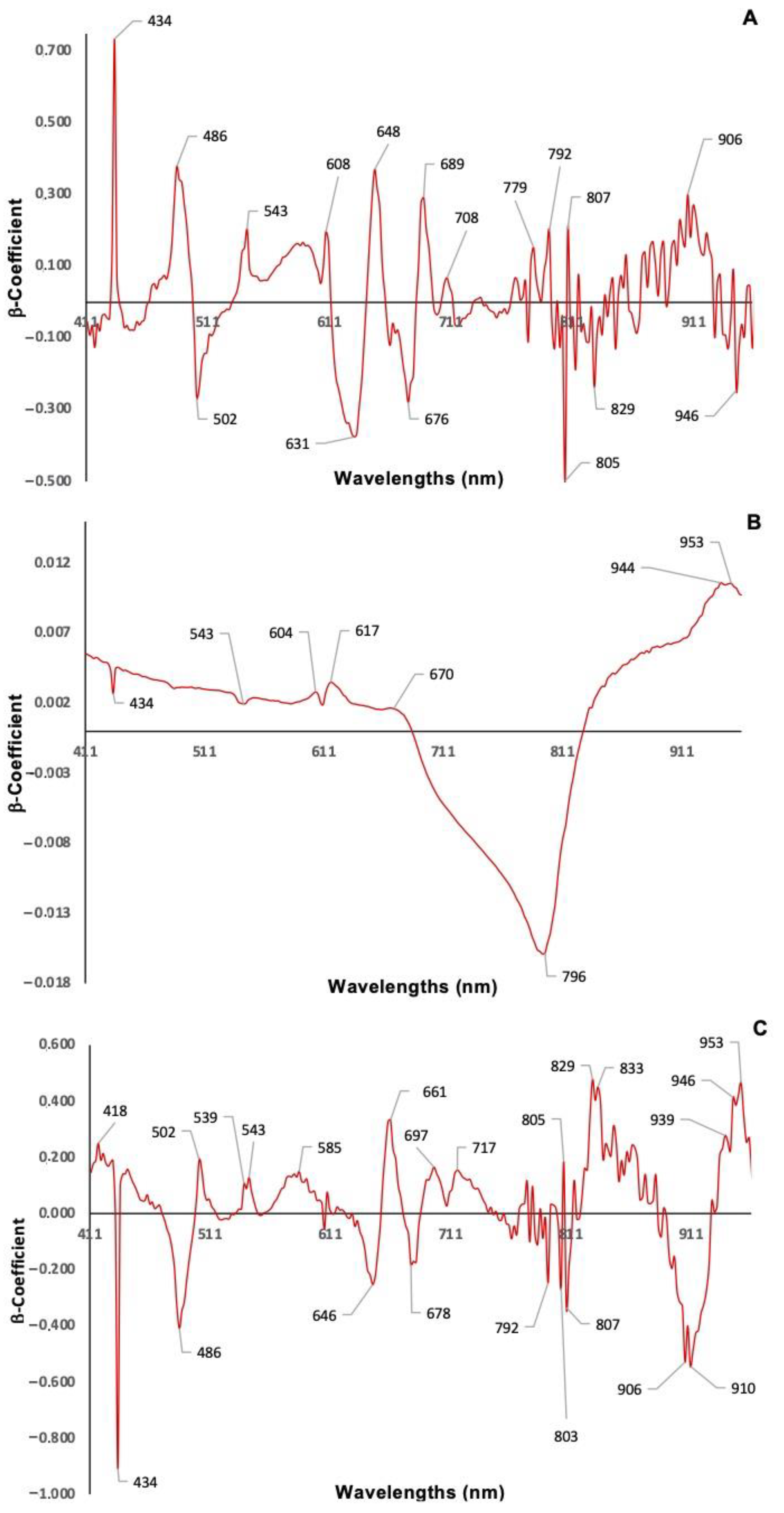
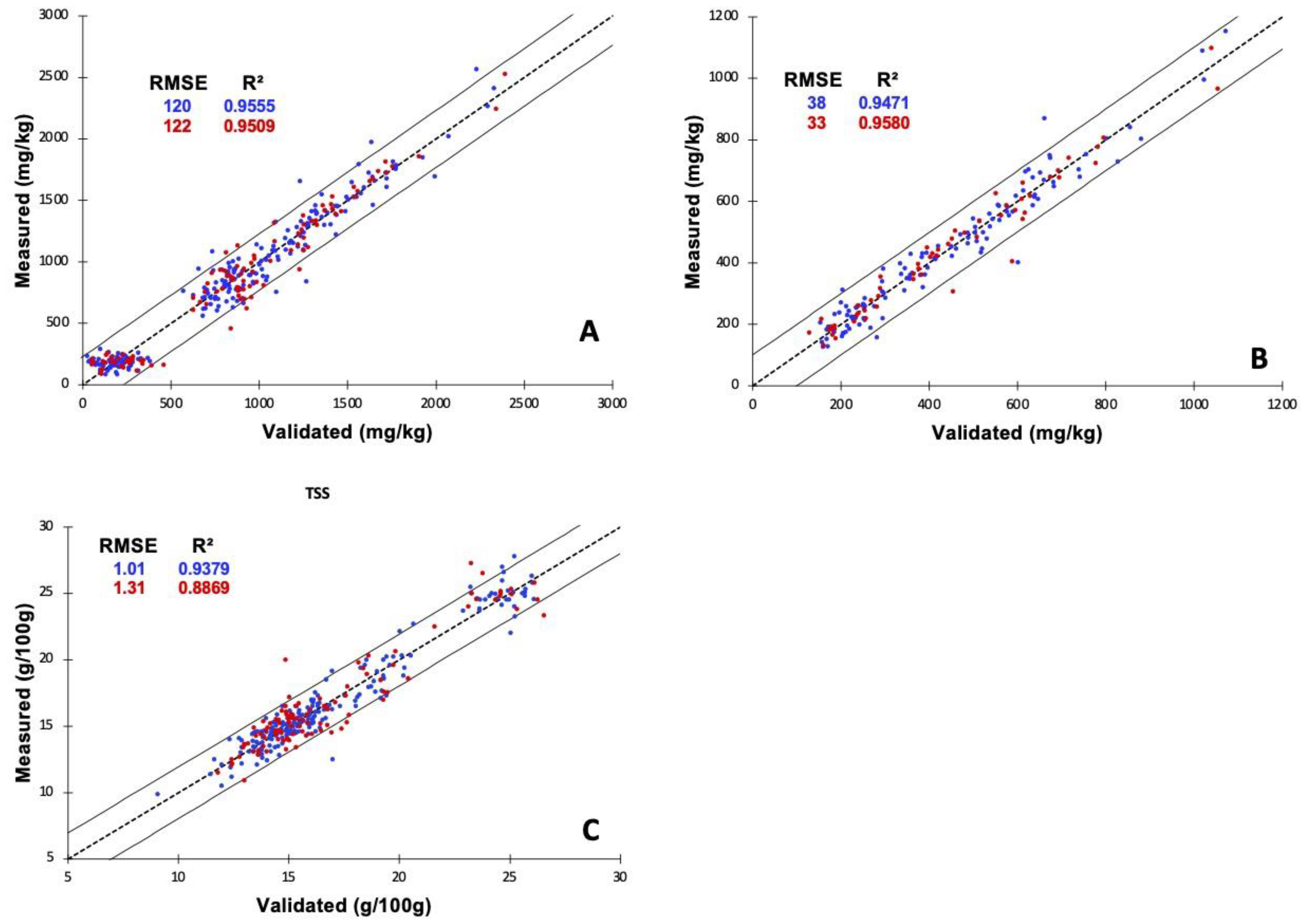
Hyperspectral data with hundreds of contiguous wavelengths for each pixel of image are a great issue for data processing. Therefore, the selection of optimal wavelengths is very important to reduce the computation time, to simplify the potential prediction model and further to satisfy the real-time inspection [52]. In this section, regression coefficients (RC) resulting from full-spectrum PLS models, were employed to select the key wavelengths aiming to establish the Multiple Linear Regression (MLR) models. Figure 4 shows the values of β-coefficients for the quality attributes Total Flavonoids, Total Anthocyanins, and TSS from the HIS data. The optimal wavelengths are those having the highest absolute values of β-coefficients (framed in the figure). Thus 17 specific wavelengths were selected for TF: 434.3, 485.5, 501.9, 543.4, 608.2, 631.4, 648.3, 675.9, 688.7, 707.9, 779, 792, 805, 807.2, 829, 905, and 945.9 nm; 8 for TA: 434.3, 543.4, 604, 616.6, 669.5, 796.3, 943.6, and 952.5 nm; and 23 for TSS: 418, 434.3, 485, 501.9, 539.2, 543.4, 585.1, 646.2, 661, 678, 697.2, 716.5, 792, 802, 805, 807.2, 829, 833, 905.9, 910.3, 939.2, 945.9, and 952.5 nm. Table 3 presents the accuracy and robustness of RC-MLR models built using the selected wavelengths. The model for TF showed R2 = 0.94 and 0.95 for the calibration and validation set respectively and RMSEV = 128 mg/kg. For TA, the model had R2cal of 0.93, R2val of 0.95 with RMSEV = 48 mg/kg, and the model for TSS presented a value of R2cal = 0.95, R2val = 0.93, and RMSEV = 1.0 g/100 g. To visualize these models, measured data vs. validated data were plotted (Figure 5). The correlation between the spectra data and the Total Flavonoid content (R²val = 0.95, Figure 5A) that of Total Anthocyanin content (R2val = 0.95, Figure 5B) and that of TSS (R2val = 0.93, Figure 5C) was good with points concentrated on the line y = x and relatively narrow scattering of data showing the low error of the model. As for Figure 3, the bimodal effect for TF and TSS was observed in Figure 5. These results seem obvious since the reduction in wavelengths for the model should not lead to a loss of information.
Thus, our models for TF, TA, and TSS showed good quantification and good prediction potential due to their RPD values (Table 3) [49,50,51]. However, the values of Bias are rather important for TA but that could be improved.
The prediction of the data from the test set showed also good results with R² over 0.93. The RMSEP obtained were in the range of RMSEC and RMSEV, with values slightly higher for TF but lower with TA and TSS.
Although the elimination of variables was approximately 92.0%, the MLR models had good performances. Compared to the full spectra, the MLR models were better for generating the model and for the prediction for TA, lower for TSS, and similar for TF. The fact that an improvement of the model is observed in some cases using MLR could be attributed to the use the optimal wavelengths neglecting unnecessary wavelengths, mitigating the problems of collinearity and overfitting [53]. Therefore, it could be demonstrated that regression coefficient algorithm is useful and effective for the selection of key wavelengths in predicting TF, TA, and TSS content in table grape.
3.5. Modelization of Table Grape Composition from Optimal Wavelengths Obtained by VIPs Score
The VIP scores resulting from the best preprocessing PLS regression model were used to develop a robust model by selection of feature-related wavelengths for TF, TA, and TSS of table grapes. The performance of the developed model by MLR depended largely on the cut-off value of the VIP scores. Generally, the “greater-than-one” rule is used to identify optimal wavelengths [54]. Only the wavelengths with highest value of VIP scores, above the threshold of 1.0, were selected to establish MLR models, whereas the wavelengths with VIP scores above 1 (spectral windows) were selected to perform a new PLS model. As shown in Figure 6, the optimal wavebands selected from all 283 wavebands were 10 (434.3, 543.4, 610.3, 633.5, 697.2, 781.1, 785.5, 805, 905.9, and 910.3 nm), 3 (710, 785.5, and 943.6 nm), and 8 (434.3, 501.9, 543.4, 610.3, 656.8, 686.5, 802.8, and 809.4 nm) for TF, TA, and TSS, respectively. Table 4 presents the accuracy and robustness of MLR models for TF, TA, and TSS based on VIP score. The model for the quality attribute TF led to R2 of 0.90 for both calibration and validation sets and with RMSEV = 178 mg/kg. The model for TA content showed R2 of 0.93 for the calibration set and 0.95 for the validation set with RMSEV = 37 mg/kg. For the sugar content (TSS), the VIPs-MLR model had R2cal equal to 0.86 and R2val of 0.83 with RMSEV = 1.6 g/100 g.
The MLR models based on the VIPs wavelengths selection showed values of RPD close or higher to 2.5, which indicated that these models were good enough to have a high utility value model [52] and was over 4 for TA showing a good prediction potential. However, these results showed a declined validation accuracy of TF and TSS models comparing to the ability of full-spectrum PLS and RC-MLR models. On the contrary, the VIPs-MLR model for TA was much better than the other with a RMSEV only of 37 mg/kg instead of 47 mg/kg in the case of the full spectra. Once more, to check the quality of the models, the measured data vs. validated data were plotted (Figure 7). All graphs showed that validated data fitted with measured data. The model is particularly good for TA with more narrow spread of the data. Again, the bimodal effect can be observed for TF and TSS. In addition, as for Figure 3, the data show that information was not lost with the reduction in wavelengths.
The prediction was good for all quality parameters (R2 > 0.86) (Table 4). The prediction errors were, however, higher for TF and TSS compared to those obtained with the full spectra and the MLR models, whereas the prediction was improved for TA.
The last trial was to select all the wavelengths with VIP score above 1 (spectral windows). New VIPs-PLS models were then build (Table 5). The VIPs-PLS model to predict TF (spectral windows: 434.3, 539.2–543.4, 608.2–610.3, 620.8–639.8, 690.8–796.3, 829, and 835.5–943.6 nm) generated a R2cal = 0.96, R2val = 0.95, and RMSEV = 122 mg/kg, using 14 LVs. The model for predicting TA content (spectral windows: 697.2–802.8 and 842.1–957 nm) was fed by 8 LVs, and generated R2cal = 0.95, R2val = 0.96, and RMSEV = 33 mg/kg. For TSS (spectral windows: 420.1, 424.1, 428.2–432.3, 436.3, 479.3–481.4, 535.1–541.3, 545.4, 555.9, 560, 564.2, 585.1–639.8, 673.8–688.7, 716.5–720.8, 864, 881.6, 890.5–892.7, 899.3, 912.5–914.8, 921.4–934.7, 939.2, and 954.8–957 nm), the VIPs-PLR model led to R2cal = 0.94, R2val = 0.89, and RMSEV = 1.3 g/100 g, using 14 LVs. RPD values suggested that all three models were good enough to quantify and predict the corresponding TF, TA, and TSS values [55]. Figure 8 shows the curves measured data vs. validated data for these best models. Again, the models fitted well with the measured data since the data spread is rather narrow for all three parameters, suggesting good validation models from specific windows HIS data. The simplified VIPs-PLS model performed with slight increase in the validation accuracy of TF and TA compared to the ability of full-spectrum PLS models, in terms of determination coefficient, RMSE, and RPD values. However, the best validation model for TSS was built using the whole spectral data.
Concerning the prediction ability of VIPs-PLS models, Table 5 showed that again the determination coefficients were over 0.94, with errors in the same range than the calibration and the validation sets. The prediction models were even better with this method using spectral windows than with the full spectra, considering both R² and RMSEP for all three quality parameters TF, TA, and TSS.
4. Discussion
The possibility to use the full spectra from HIS to generate a relevant PLS-model to predict the sugar content was indeed reported by Baiano et al. [47] using the same device. These authors developed a calibration models able to predict TSS of white and red table grape with R2val of 0.94 and 0.93, respectively. Our method was, however, valid for all grape varieties, with all reds, rosés, and whites, which would be easier to manage from an industrial point of view. In addition, the results of the present study were comparable to those of another work carried out by Gomes et al. [56], in which the prediction of TSS in wine grape was performed using two different model development techniques, i.e., PLS regression and Neural Networks. The obtained values of R2 of prediction were 0.92 for both PLS regression and Neural Networks with RMSEP of 0.94°Brix and 0.96°Brix, respectively. Hence, a good capacity of correlation was achieved in numerous other works on prediction of TSS for table and wine grapes [24,38,57,58].
Other authors have also reported good performance of linear models to predict the total anthocyanin content, with R2CV > 0.94 using spectral data in Vis-NIR [59] and NIR ranges [60] or total phenols content, with R2CV = 0.89 using the spectral data in Vis-NIR range [57,61]. Moreover, several studies also reported very good performance of nonlinear models to predict the TA content in whole Port and Cabernet sauvignon wine grape using the hyperspectral imaging device in Vis–NIR range [38,56,62]. Thus, our results were at least as good as those of other works but for the first time showed the relevance of HIS on red and white table grapes.
Our results highlighted that not only hyperspectral imaging is a relevant method to assess TA, TF, and TSS content but also the reduction in data is possible using MLR method with β-coefficients (RC method) or variable importance in the projection VIP. RC methods were already reported to be relevant to predict sugar content in the case of lychee fruit [55] and the total polyphenols concentration in cocoa beans [60,63]. Sen and co-workers [64] have also applied VIP selection to build OPLS models for the prediction of chemical parameters of wine by combined use of visible and mid-infrared (MIR) spectroscopies. These authors have built models able to predict anthocyanin compounds, total phenol content, and TSS of red wine with R2val ranging between 0.77 and 0.96.
The use of VIP in a PLR model (specific windows) was applied by Sen and co-workers [64] to build OPLS models for the prediction of chemical parameters of wine by combined use of visible and mid-infrared (MIR) spectroscopies. These authors have built models able to predict anthocyanin compounds, total phenol content, and TSS of red wine with R2val ranging between 0.77 and 0.96. Our work is thus in adequation with the previous studies and showed for the first time that reducing data, thanks to VIP or β-coefficients from HIS, is suitable for table grapes. No similar results have been found in table grapes for the control of Total Flavonoids and the Total Anthocyanins, although they have been found in wine grapes and other matrices with errors of the same order of magnitude [24,59,60,65].
Looking now at the other quality factor of a calibration model, the measurement of TSS by refractometry led to a standard deviation ≤ 1.8 (Table 1) in which was included the incertitude due to the refractometer and to the heterogeneity of the berries. Using full spectra, the PLS model only led to a RMSEP of 0.9. The reduction in the number of wavelengths reduced it to 0.7°Brix for β-coefficients wavelength selection. For TA, the lowest RMSEP was obtained thanks to VIPs-PLS (27 mg/kg), followed by both full spectra and VIPs-MLR from optimal wavelengths (33 mg/kg). For TF, the prediction models are much better for high level of flavonoid content. RMSEP decreased from 374 mg/kg (reference method, Table 1) to 128 mg/kg with VIPs score with specific windows or 149 mg/kg with β-coefficients. However, for very low concentration of flavonoids, like the Victoria variety, the models induced higher RMSEP.
Hyperspectral imaging is a tool, which could provide relevant on-line information about Total Flavonoid, Total Anthocyanins, and Total Soluble Solids through the use of consistent validation models. The models from the full spectra generated by SNV pre-treatment and the fact that the models were built using grape berries of seven different cultivar contributed to the robustness of our models. The possibility to use the same pre-treatment for all parameters and all varieties is interesting and could limit the complexity of the method and avoid mistakes in a professional use.
The reduction in data using only the wavelength with highest β-coefficient (absolute values) from one side, and spectral windows obtained from all the wavelengths with VIPs > 1 on another side, would allow an industrial use needing less computer data memory and quicker answers. That method could be used also as quality control. Database has first to be expanded not only to strength our current models but also to test new non-linear models. Another step would be to implement hyperspectral imaging on an industrial conveyor belt to take into account not only elements such as vibration on the conveyor but also analytical speed to provide real-time information. Moreover, in an on-line perspective, the localized information could be added for separating berries from a batch in order to get two or several final batches for different transformations or different quality array, depending on berry average spectrum, thus, on their composition. Nonetheless, that tool could anyway be used for a rapid table grape characterization in producer or industry places.
Author Contributions
Conceptualization, M.G.; methodology, M.G. and P.P.; validation, P.P.; formal analysis, M.G.; investigation, V.L.-V., M.G., and C.M.; resources, V.L.-V.; data curation, M.G.; writing—original draft preparation, M.G. and C.M.; writing—review and editing, C.M., M.G., and P.P.; visualization, C.M.; supervision, C.M.; project administration, C.M.; funding acquisition, C.M. All authors have read and agreed to the published version of the manuscript.
Funding
This research was conducted in the framework of the regional program “Objectif Végétal, Research, Education and Innovation in Pays de la Loire,” supported by the French Region Pays de la Loire, Angers Loire Métropole, and the European Regional Development Fund. The chemiometry was realized thanks to Region Pays de la Loire and Interprofession des Vins du Val de Loire InterLoire in the frame of the O3VINS project.
Institutional Review Board Statement
Not applicable.
Informed Consent Statement
Not applicable.
Data Availability Statement
Not applicable.
Acknowledgments
Authors want to thank Dominique Le Meurlay for logistic support and Susana Pombo for English language check.
Conflicts of Interest
The authors declare no conflict of interest.
References
- International Organisation of Vine and Wine (OIV). Statistical Report on World Vitiviniculture. 2019. Available online: http://www.oiv.int/public/medias/6782/oiv-2019-statistical-report-on-world-vitiviniculture.pdf (accessed on 12 January 2021).
- Valero, D.; Valverde, J.; Martínez-Romero, D.; Guillén, F.; Castillo, S.; Serrano, M. The combination of modified atmosphere packaging with eugenol or thymol to maintain quality, safety and functional properties of table grapes. Postharvest Biol. Technol. 2006, 41, 317–327. [Google Scholar] [CrossRef]
- Hellín, P.; Manso, A.; Flores, P.; Fenoll, J. Evolution of Aroma and Phenolic Compounds during Ripening of ’Superior Seedless’ Grapes. J. Agric. Food Chem. 2010, 58, 6334–6340. [Google Scholar] [CrossRef]
- Zeppa, G.; Rolle, L.; Gerbi, V. Valutazione mediante consumer test dell’attitudine al consumo diretto di un’uva a bacca rossa. Indus. Alim. 1999, 38, 818–824. [Google Scholar]
- Piva, C.R.; Garcia, J.L.L.; Morgan, W. The ideal table grapes for the Spanish market. Rev. Bras. Frutic. 2006, 28, 258–261. [Google Scholar] [CrossRef] [Green Version]
- Abdullah, M.; Guan, L.; Lim, K.; Karim, A. The applications of computer vision system and tomographic radar imaging for assessing physical properties of food. J. Food Eng. 2004, 61, 125–135. [Google Scholar] [CrossRef]
- Turati, F.; Rossi, M.; Pelucchi, C.; Levi, F.; La Vecchia, C. Fruit and vegetables and cancer risk: A review of southern European studies. Br. J. Nutr. 2015, 113, S102–S110. [Google Scholar] [CrossRef]
- Vieira, A.R.; Abar, L.; Vingeliene, S.; Chan, D.S.M.; Aune, D.; Navarro-Rosenblatt, D.; Stevens, C.; Greenwood, D.; Norat, T. Fruits, vegetables and lung cancer risk: A systematic review and meta-analysis. Ann. Oncol. 2016, 27, 81–96. [Google Scholar] [CrossRef]
- Perestrelo, R.; Silva, C.; Pereira, J.; Câmara, J.S. Healthy effects of bioactive metabolites from Vitis vinifera L. grapes: A review. In Grapes: Production, Phenolic Composition and Potential Biomedical Effects; Câmara, J.S., Ed.; Nova Science Technology: Hauppauge, NY, USA, 2014; pp. 305–338. [Google Scholar]
- Shahidi, F.; Ambigaipalan, P. Phenolics and polyphenolics in foods, beverages and spices: Antioxidant activity and health effects–A review. J. Funct. Foods 2015, 18, 820–897. [Google Scholar] [CrossRef]
- Basile, T.; Alba, V.; Gentilesco, G.; Savino, M.; Tarricone, L. Anthocyanins pattern variation in relation to thinning and girdling in commercial Sugrathirteen® table grape. Sci. Hortic. 2018, 227, 202–206. [Google Scholar] [CrossRef]
- Río Segade, S.; Giacosa, S.; Torchio, F.; De Palma, L.; Novello, V.; Gerbi, V.; Rolle, L. Impact of different advanced ripening stages on berry texture properties of ‘Red Globe’ and ‘Crimson Seedless’ table grape cultivars (Vitis vinifera L.). Sci. Hortic. 2013, 160, 313–319. [Google Scholar] [CrossRef]
- Kontoudakis, N.; Esteruelas, M.; Fort, F.; Canals, J.M.; Zamora, F. Comparison of methods for estimating phenolic maturity in grapes: Correlation between predicted and obtained parameters. Anal. Chim. Acta 2010, 660, 127–133. [Google Scholar] [CrossRef]
- Mota, A.; Pinto, J.; Fartouce, I.; Correia, M.J.; Costa, R.; Carvalho, R.; Aires, A.; Oliveira, A.A. Chemical profile and antioxidant potential of four table grape (Vitis vinifera) cultivars grown in Douro region, Portugal. Ciência Técnica Vitivinícola 2018, 33, 125–135. [Google Scholar] [CrossRef]
- Zhao, Y.; Zhang, C.; Zhu, S.; Gao, P.; Feng, L.; He, Y. Non-Destructive and Rapid Variety Discrimination and Visualization of Single Grape Seed Using Near-Infrared Hyperspectral Imaging Technique and Multivariate Analysis. Molecules 2018, 23, 1352. [Google Scholar] [CrossRef] [Green Version]
- Fragoso, S.; Mestres, M.; Busto, O.; Guasch, J. Comparison of Three Extraction Methods Used to Evaluate Phenolic Ripening in Red Grapes. J. Agric. Food Chem. 2010, 58, 4071–4076. [Google Scholar] [CrossRef]
- Costa, G.; Noferini, M.; Fiori, G.; Torrigiani, P. Use of vis/nir spectroscopy to assess fruit ripening stage and improve management in post-harvest chain. Fresh Prod. 2009, 3, 35–41. [Google Scholar]
- Arendse, E.; Fawole, O.A.; Magwaza, L.S.; Opara, U.L. Non-destructive prediction of internal and external quality attributes of fruit with thick rind: A review. J. Food Eng. 2018, 217, 11–23. [Google Scholar] [CrossRef]
- Whitacre, E.; OLiver, J.; Broek, R.; Engelen, P.; Remers, B.K.; Horst, B.; Tewart, M.S.; Jansen-Beuvink, A. Predictive Analysis of Cocoa Procyanidins Using Near-Infrared Spectroscopy Techniques. J. Food Sci. 2003, 68, 2618–2622. [Google Scholar] [CrossRef]
- Chen, Q.; Zhao, J.; Liu, M.; Cai, J.; Liu, J. Determination of total polyphenols content in green tea using FT-NIR spectroscopy and different PLS algorithms. J. Pharm. Biomed. Anal. 2008, 46, 568–573. [Google Scholar] [CrossRef]
- Cozzolino, D.; Kwiatkowski, M.J.; Parker, M.; Cynkar, W.U.; Dambergs, R.G.; Gishen, M.; Herderich, M.J. Prediction of phenolic compounds in red wine fermentations by visible and near infrared spectroscopy. Anal. Chim. Acta 2004, 513, 73–80. [Google Scholar] [CrossRef]
- Versari, A.; Parpinello, G.P.; Mattioli, A.U.; Galassi, S. Determination of grape quality at harvest using Fourier-transform mid-infrared spectroscopy and multivariate analysis. Am. J. Enol. Vitic. 2008, 59, 317–322. [Google Scholar]
- Cozzolino, D.; Cynkar, W.U.; Dambergs, R.G.; Mercurio, M.D.; Smith, P.A. Measurement of Condensed Tannins and Dry Matter in Red Grape Homogenates Using Near Infrared Spectroscopy and Partial Least Squares. J. Agric. Food Chem. 2008, 56, 7631–7636. [Google Scholar] [CrossRef]
- Pathmanaban, P.; Gnanavel, B.; Anandan, S.S. Recent application of imaging techniques for fruit quality assessment. Trends Food Sci. Technol. 2019, 94, 32–42. [Google Scholar] [CrossRef]
- Ma, J.; Sun, D.-W.; Pu, H.; Cheng, J.-H.; Wei, Q. Advanced Techniques for Hyperspectral Imaging in the Food Industry: Principles and Recent Applications. Annu. Rev. Food Sci. Technol. 2019, 10, 197–220. [Google Scholar] [CrossRef] [PubMed]
- Cen, H.; Lu, R.; Ariana, D.P.; Mendoza, F. Hyperspectral imaging-based classification and wavebands selection for internal defect detection of pickling cucumbers. Food Bioproc. Technol. 2013, 7, 1689–1700. [Google Scholar] [CrossRef]
- Torres, I.; Amigo, J.-M. An overview of regression methods in hyperspectral and multispectral imaging. Data Handl. Sci. Technol. 2020, 32, 205–230. [Google Scholar] [CrossRef]
- Elmasry, G.; Kamruzzaman, M.; Sun, D.-W.; Allen, P. Principles and Applications of Hyperspectral Imaging in Quality Evaluation of Agro-Food Products: A Review. Crit. Rev. Food Sci. Nutr. 2012, 52, 999–1023. [Google Scholar] [CrossRef]
- Qin, J.; Kim, M.S.; Chao, K.; Chan, D.E.; Delwiche, S.R.; Cho, B.-K. Line-Scan Hyperspectral Imaging Techniques for Food Safety and Quality Applications. Appl. Sci. 2017, 7, 125. [Google Scholar] [CrossRef] [Green Version]
- Siche, R.; Vejarano, R.; Aredo, V.; Velasquez, L.; Saldaña, E.; Quevedo, R. Evaluation of Food Quality and Safety with Hyperspectral Imaging (HSI). Food Eng. Rev. 2016, 8, 306–322. [Google Scholar] [CrossRef]
- Wu, D.; Sun, D.-W. Advanced applications of hyperspectral imaging technology for food quality and safety analysis and assessment: A review—Part II: Applications. Innov. Food Sci. Emerg. Technol. 2013, 19, 15–28. [Google Scholar] [CrossRef]
- Feng, L.; Zhu, S.; Zhang, C.; Bao, Y.; Gao, P.; He, Y. Variety Identification of Raisins Using Near-Infrared Hyperspectral Imaging. Molecules 2018, 23, 2907. [Google Scholar] [CrossRef] [Green Version]
- Calvini, R.; Ulrici, A.; Amigo, J.M. Practical comparison of sparse methods for classification of Arabica and Robusta coffee species using near infrared hyperspectral imaging. Chemom. Intell. Lab. Syst. 2015, 146, 503–511. [Google Scholar] [CrossRef] [Green Version]
- Chandrasekaran, I.; Panigrahi, S.S.; Ravikanth, L.; Singh, C.B. Potential of Near-Infrared (NIR) Spectroscopy and Hyperspectral Imaging for Quality and Safety Assessment of Fruits: An Overview. Food Anal. Methods 2019, 12, 2438–2458. [Google Scholar] [CrossRef]
- Pu, Y.-Y.; Feng, Y.-Z.; Sun, D.-W. Recent Progress of Hyperspectral Imaging on Quality and Safety Inspection of Fruits and Vegetables: A Review. Compr. Rev. Food Sci. Food Saf. 2015, 14, 176–188. [Google Scholar] [CrossRef]
- Gowen, A.; Odonnell, C.; Cullen, P.; Downey, G.; Frias, J. Hyperspectral imaging–an emerging process analytical tool for food quality and safety control. Trends Food Sci. Technol. 2007, 18, 590–598. [Google Scholar] [CrossRef]
- Taghizadeh, M.; Gowen, A.A.; O’Donnell, C.P. Comparison of hyperspectral imaging with conventional RGB imaging for quality evaluation of Agaricus bisporus mushrooms. Biosyst. Eng. 2011, 108, 191–194. [Google Scholar] [CrossRef]
- Fernandes, A.M.; Franco, C.; Mendes-Ferreira, A.; Mendes-Faia, A.; Da Costa, P.L.; Melo-Pinto, P. Brix, pH and anthocyanin content determination in whole Port wine grape berries by hyperspectral imaging and neural networks. Comput. Electron. Agric. 2015, 115, 88–96. [Google Scholar] [CrossRef]
- Tallada, J.G.; Bato, P.M.; Shrestha, B.P.; Kobayashi, T.; Nagata, M. Quality evaluation of plant products. In Hyperspectral Imaging Technology in Food and Agriculture; Park, B., Lu, R., Eds.; Springer: New York, NY, USA, 2015; pp. 227–249. [Google Scholar]
- Fracassetti, D.; Gabrielli, M.; Corona, O.; Tirelli, A. Characterisation of Vernaccia Nera (Vitis vinifera L.) grapes and wine. S. Afr. J. Enol. Vitic. 2017, 38, 72–81. [Google Scholar]
- Lee, J.; Kang, H. Flood fill mean shift: A robust segmentation algorithm. Int. J. Control. Autom. Syst. 2010, 8, 1313–1319. [Google Scholar] [CrossRef]
- Picouet, P.A.; Gou, P.; Hyypiö, R.; Castellari, M. Implementation of NIR technology for at-line rapid detection of sunflower oil adulterated with mineral oil. J. Food Eng. 2018, 230, 18–27. [Google Scholar] [CrossRef]
- Stchur, P.; Cleveland, D.; Zhou, J.; Michel, R.G. A review of recent applications of near infrared spectroscopy, and of the characteristics of a novel pbs ccd array-based near-infrared spectrometer. Appl. Spectrosc. Rev. 2002, 37, 383–428. [Google Scholar] [CrossRef]
- Rajkumar, P.; Wang, N.; Eimasry, G.; Raghavan, G.; Gariepy, Y. Studies on banana fruit quality and maturity stages using hyperspectral imaging. J. Food Eng. 2012, 108, 194–200. [Google Scholar] [CrossRef]
- Olah, M.; Bologa, C.; Oprea, T.I. An automated PLS search for biologically relevant QSAR descriptors. J. Comput. Mol. Des. 2004, 18, 437–449. [Google Scholar] [CrossRef] [Green Version]
- Mikulic-Petkovsek, M.; Skvarc, A.; Rusjan, D. Biochemical composition of different table grape cultivars produced in Slovenia. J. Hortic. Sci. Biotechnol. 2018, 94, 368–377. [Google Scholar] [CrossRef]
- Baiano, A.; Terracone, C.; Peri, G.; Romaniello, R. Application of hyperspectral imaging for prediction of physico-chemical and sensory characteristics of table grapes. Comput. Electron. Agric. 2012, 87, 142–151. [Google Scholar] [CrossRef]
- Costa, D.D.S.; Mesa, N.F.O.; Freire, M.S.; Ramos, R.P.; Mederos, B.J.T. Development of predictive models for quality and maturation stage attributes of wine grapes using vis-nir reflectance spectroscopy. Postharvest Biol. Technol. 2019, 150, 166–178. [Google Scholar] [CrossRef]
- Yang, Q.; Sun, D.-W.; Cheng, W. Development of simplified models for nondestructive hyperspectral imaging monitoring of TVB-N contents in cured meat during drying process. J. Food Eng. 2017, 192, 53–60. [Google Scholar] [CrossRef]
- De Marchi, M.; Fagan, C.; O’Donnell, C.; Cecchinato, A.; Zotto, R.D.; Cassandro, M.; Penasa, M.; Bittante, G. Prediction of coagulation properties, titratable acidity, and pH of bovine milk using mid-infrared spectroscopy. J. Dairy Sci. 2009, 92, 423–432. [Google Scholar] [CrossRef]
- Gherardi Hein, P.R.; Maioli Campos, A.C.; Trugilho, P.F.; Lima, J.T.; Chaix, G. Near infrared spectroscopy for estimating wood basic density in Eucalyptus urophylla and E. grandis. Cerne 2009, 15, 133–141. [Google Scholar]
- Pu, H.; Kamruzzaman, M.; Sun, D.-W. Selection of feature wavelengths for developing multispectral imaging systems for quality, safety and authenticity of muscle foods—A review. Trends Food Sci. Technol. 2015, 45, 86–104. [Google Scholar] [CrossRef]
- Galvão, R.K.H.; Araújo, M.C.U.; Fragoso, W.D.; Silva, E.C.; José, G.E.; Soares, S.F.C.; Paiva, H.M. A variable elimination method to improve the parsimony of MLR models using the successive projections algorithm. Chemom. Intell. Lab. Syst. 2008, 92, 83–91. [Google Scholar] [CrossRef]
- Andersen, C.M.; Bro, R. Variable selection in regression—A tutorial. J. Chemom. 2010, 24, 728–737. [Google Scholar] [CrossRef]
- Pu, H.; Liu, D.; Wang, L.; Sun, D.-W. Soluble Solids Content and pH Prediction and Maturity Discrimination of Lychee Fruits Using Visible and Near Infrared Hyperspectral Imaging. Food Anal. Methods 2016, 9, 235–244. [Google Scholar] [CrossRef]
- Gomes, V.M.; Fernandes, A.M.; Faia, A.; Melo-Pinto, P. Comparison of different approaches for the prediction of sugar content in new vintages of whole Port wine grape berries using hyperspectral imaging. Comput. Electron. Agric. 2017, 140, 244–254. [Google Scholar] [CrossRef]
- Nogales-Bueno, J.; Hernández-Hierro, J.M.; Rodríguez-Pulido, F.J.; Heredia, F.J. Determination of technological maturity of grapes and total phenolic compounds of grape skins in red and white cultivars during ripening by near infrared hyperspectral image: A preliminary approach. Food Chem. 2014, 152, 586–591. [Google Scholar] [CrossRef] [PubMed]
- Piazzolla, F.; Amodio, M.L.; Colelli, G. Spectra evolution over on-vine holding of Italia table grapes: Prediction of maturity and discrimination for harvest times using a Vis-NIR hyperspectral device. J. Agric. Eng. 2017, 48, 109–116. [Google Scholar] [CrossRef] [Green Version]
- Diago, M.P.; Fernández-Novales, J.; Fernandes, A.M.; Melo-Pinto, P.; Tardaguila, J. Use of Visible and Short-Wave Near-Infrared Hyperspectral Imaging to Fingerprint Anthocyanins in Intact Grape Berries. J. Agric. Food Chem. 2016, 64, 7658–7666. [Google Scholar] [CrossRef]
- Chen, S.; Zhang, F.; Ning, J.; Liu, X.; Zhang, Z.; Yang, S. Predicting the anthocyanin content of wine grapes by NIR hyperspectral imaging. Food Chem. 2015, 172, 788–793. [Google Scholar] [CrossRef]
- Nogales-Bueno, J.; Baca-Bocanegra, B.; Rodríguez-Pulido, F.J.; Heredia, F.J.; Hernández-Hierro, J.M. Use of near infrared hyperspectral tools for the screening of extractable polyphenols in red grape skins. Food Chem. 2015, 172, 559–564. [Google Scholar] [CrossRef] [Green Version]
- Fernandes, A.M.; Oliveira, P.; Moura, J.P.; Oliveira, A.A.; Falco, V.; Correia, M.J.; Melo-Pinto, P. Determination of anthocyanin concentration in whole grape skins using hyperspectral imaging and adaptive boosting neural networks. J. Food Eng. 2011, 105, 216–226. [Google Scholar] [CrossRef]
- Caporaso, N.; Whitworth, M.B.; Fowler, M.S.; Fisk, I.D. Hyperspectral imaging for non-destructive prediction of fermentation index, polyphenol content and antioxidant activity in single cocoa beans. Food Chem. 2018, 258, 343–351. [Google Scholar] [CrossRef]
- Sen, I.; Ozturk, B.; Tokatli, F.; Ozen, B. Combination of visible and mid-infrared spectra for the prediction of chemical parameters of wines. Talanta 2016, 161, 130–137. [Google Scholar] [CrossRef] [PubMed] [Green Version]
- Dambergs, R.; Gishen, M.; Cozzolino, D. A Review of the State of the Art, Limitations, and Perspectives of Infrared Spectroscopy for the Analysis of Wine Grapes, Must, and Grapevine Tissue. Appl. Spectrosc. Rev. 2015, 50, 261–278. [Google Scholar] [CrossRef]
Figure 1.
Hyperspectral imaging system: (a) a charge-coupled device (CCS) camera, (b) a spectrograph with a standard C-mount zoom lens, (c) quartz tungsten halogen (QTH) lighting unit, (d) translation stage, and (e) a PC with image acquisition software.
Figure 1.
Hyperspectral imaging system: (a) a charge-coupled device (CCS) camera, (b) a spectrograph with a standard C-mount zoom lens, (c) quartz tungsten halogen (QTH) lighting unit, (d) translation stage, and (e) a PC with image acquisition software.

Figure 2.
Mean reflectance spectra profiles obtained by hyperspectral imaging spectroscopy. Sable Seedless (dark blue), Seedless Sugarone (red), Alphonse Lavallée (green), Thompson Seedless (purple), Lival (turquoise), Black Magic (orange), and Vittoria (clear blue) table grapes samples.
Figure 2.
Mean reflectance spectra profiles obtained by hyperspectral imaging spectroscopy. Sable Seedless (dark blue), Seedless Sugarone (red), Alphonse Lavallée (green), Thompson Seedless (purple), Lival (turquoise), Black Magic (orange), and Vittoria (clear blue) table grapes samples.

Figure 3.
Performance of partial least square (PLS) model using the spectral data pre-treated by SNV. Calibration and external validation for total flavonoids using 9 factors (A), for Total Anthocyanins using 3 factors (B), and for Total Soluble Solids using 10 factors (C). Blue dots indicate calibration set and red dots represent validation set. R2: determination coefficient, RMSE: root mean squared error.

Figure 4.
Values of β-coefficients for all wavelengths for predicting quality attributes in table grape for the quality attributes, Total Flavonoids (A), Total Anthocyanins (B), and Total Soluble Solids (TSS) (C).
Figure 4.
Values of β-coefficients for all wavelengths for predicting quality attributes in table grape for the quality attributes, Total Flavonoids (A), Total Anthocyanins (B), and Total Soluble Solids (TSS) (C).

Figure 5.
Performance of Multiple Linear Regression (MLR) models using only the optimal wavelengths extracted from β-coefficients of PLS analysis. Calibration and external validation using SNV pre-treated data: (A) for Total Flavonoids, (B) for Total Anthocyanins, and (C) for TSS. Blue dots indicate calibration set and black dots represent validation set.

Figure 6.
Values of Variable Importance in Projections (VIP) scores for all wavelengths for predicting quality attributes in table grape for the quality attributes Total Flavonoids (A), Total Anthocyanins (B), and Total Soluble Solids TSS (C).
Figure 6.
Values of Variable Importance in Projections (VIP) scores for all wavelengths for predicting quality attributes in table grape for the quality attributes Total Flavonoids (A), Total Anthocyanins (B), and Total Soluble Solids TSS (C).

Figure 7.
Performance of MLR model using the optimal wavelengths extracted from VIPs score of the best full-spectrum PLS analysis. Calibration and external validation from SNV pre-treated data for (A) Total Flavonoids, (B) Total Anthocyanins, and (C) Total Soluble Solids. Blue dots indicate calibration set and red dots represent validation set.

Figure 8.
Performance of PLS model using the optimal wavelength windows extracted from VIPs score (>1) of PLS analysis. Calibration and external validation for (A) Total Flavonoids, (B) Total Anthocyanins, and (C) Total Soluble Solids. Blue dots indicate calibration set and red dots represent validation set.


Table 1.
Grape composition. Total Anthocyanins (TA), Total Flavonoids (TF) Content, and Total Soluble Solids (TSS) of table grapes. a b c, and d letters within the same column indicate significant differences among table grape cultivars according to Tukey-b test (p < 0.05). FW: fresh weight.
Table 1.
Grape composition. Total Anthocyanins (TA), Total Flavonoids (TF) Content, and Total Soluble Solids (TSS) of table grapes. a b c, and d letters within the same column indicate significant differences among table grape cultivars according to Tukey-b test (p < 0.05). FW: fresh weight.
| Grape Cultivars | Origin | TF (mg kg−1 F) | TA (mg kg−1 FM) | TSS (g 100 g−1) |
|---|---|---|---|---|
| Sable Seedless | South Africa | 1131 ± 267 c | 590 ± 163 a | 19.0 ± 1.8 b |
| Alphonse Lavallée | South Africa | 829 ± 153 d | 217 ± 61 c | 24.8 ± 1.1 a |
| Lival | France | 1642 ± 374 a | 588 ± 222 a | 15.0 ± 1.7 cd |
| Black Magic | Italy | 1279 ± 259 b | 399 ± 132 b | 15.4 ± 0.9 c |
| Sugarone Superior Seedless | South Africa | 162 ± 43 e | 0 | 14.7 ± 1.0 d |
| Thompson Seedless | Egypt | 826 ± 136 d | 0 | 15.5 ± 1.9 c |
| Victoria | Italy | 201 ± 28 e | 0 | 14.0 ± 1.5 e |
| p < 0.001 | p < 0.001 | p < 0.001 |
Table 2.
Performance of partial least square (PLS) models depending on data pre-treatments for predicting TF, TA, and SSC, using full spectra (400–1000 nm). TF: Total Flavonoids, TA: Total Anthocyanins and TSS: Total Soluble Solids, WD: white and black correction, der: derivative, SNV: Standard Normal Variate. LVs: number of latent variables.
| Variable | Pre-Treatment | LVs | Calibration Set | Validation Set | Prediction Set | |||||
|---|---|---|---|---|---|---|---|---|---|---|
| R2c | RMSEC | R2val | RMSEV | BIAS | RPD | R2pr | RMSEP | |||
| TF | SNV | 9 | 0.94 | 146 | 0.93 | 141 | −9.45 | 3.90 | 0.92 | 159 |
| 1st DER | 9 | 0.95 | 128 | 0.93 | 148 | 5.2 | 3.70 | 0.96 | 120 | |
| WD | 12 | 0.94 | 134 | 0.94 | 132 | −0.13 | 4.16 | 0.95 | 130 | |
| 2nd DER | 5 | 0.93 | 149 | 0.89 | 183 | 13.0 | 3.01 | 0.89 | 196 | |
| TA | SNV | 3 | 0.93 | 59 | 0.95 | 47 | 6.7 | 4.61 | 0.98 | 33 |
| 1st DER | 4 | 0.93 | 61 | 0.92 | 56 | 6.8 | 3.87 | 0.97 | 39 | |
| WD | 6 | 0.91 | 65 | 0.93 | 56 | 5.0 | 3.90 | 0.97 | 41 | |
| 2nd DER | 4 | 0.90 | 70 | 0.91 | 65 | 14.0 | 3.32 | 0.96 | 50 | |
| TSS | SNV | 10 | 0.94 | 1.0 | 0.91 | 1.1 | −0.05 | 3.45 | 0.95 | 0.9 |
| 1st DER | 6 | 0.93 | 1.0 | 0.91 | 1.2 | −0.07 | 3.33 | 0.93 | 1.1 | |
| WD | 15 | 0.96 | 0.8 | 0.94 | 0.9 | 0.01 | 4.17 | 0.96 | 0.8 | |
| 2nd DER | 5 | 0.92 | 1.1 | 0.88 | 1.4 | −0.01 | 2.90 | 0.92 | 1.1 | |
Table 3.
Multiple Linear Regression (MLR) model performance for Total Flavonoids (TF), Total Anthocyanins (TA) and Total Soluble Solids (TSS) from optimal wavelengths selection based on β-coefficient of the best PLS full spectra analysis.
Table 3.
Multiple Linear Regression (MLR) model performance for Total Flavonoids (TF), Total Anthocyanins (TA) and Total Soluble Solids (TSS) from optimal wavelengths selection based on β-coefficient of the best PLS full spectra analysis.
| Variable | Optimal Wavelengths (nm) | Calibration Set | Validation Set | Prediction Set | |||||
|---|---|---|---|---|---|---|---|---|---|
| R2c | RMSEC | R2val | RMSEV | Bias | RPD | R2pr | RMSEP | ||
| TF | 434.3, 485.5, 501.9, 543.4, 608.2, 631.4, 648.3, 675.9, 688.7, 707.9, 779, 792, 805, 807.2, 829, 905, 945.9 | 0.94 | 136 | 0.95 | 128 | 0.9 | 4.27 | 0.93 | 149 |
| TA | 434.3, 543.4, 604, 616.6, 669.5, 796.3, 943.6, 952.5 | 0.93 | 55 | 0.95 | 48 | 4.5 | 4.51 | 0.97 | 39 |
| TSS | 418, 434.3, 485, 501.9, 539.2, 543.4, 585.1, 646.2, 661, 678, 697.2, 716.5, 792, 802, 805, 807.2, 829, 833, 905.9, 910.3, 939.2, 945.9, 952.5 | 0.95 | 0.9 | 0.93 | 1.0 | −0.06 | 3.82 | 0.97 | 0.7 |
Table 4.
Performance of MLR models for predicting Total Flavonoids (TF), Total Anthocyanins (TA), and the Total Soluble Solids (TSS) using the optimal wavelengths extracted from VIPs of the best PLS full spectra analysis.
Table 4.
Performance of MLR models for predicting Total Flavonoids (TF), Total Anthocyanins (TA), and the Total Soluble Solids (TSS) using the optimal wavelengths extracted from VIPs of the best PLS full spectra analysis.
| Variable | Optimal Wavelengths (nm) | Calibration Set | Validation Set | Prediction Set | |||||
|---|---|---|---|---|---|---|---|---|---|
| R2c | RMSEC | R2val | RMSEV | Bias | RPD | R2pr | RMSEP | ||
| TF | 434.3, 543.4, 610.3, 633.5, 697.2, 781.1, 785.5, 805, 905.9, 910.3 | 0.90 | 178 | 0.90 | 178 | −11.3 | 3.09 | 0.93 | 155 |
| TA | 710, 785.5, 943.6 | 0.93 | 44 | 0.95 | 37 | 5.6 | 5.90 | 0.98 | 33 |
| TSS | 434.3, 501.9, 543.4, 610.3, 656.8, 686.5, 802.8, 809.4 | 0.86 | 1.5 | 0.83 | 1.6 | −0.06 | 2.46 | 0.86 | 1.4 |
Table 5.
Performance of Variable Importance in Projections (VIPs)-PLS models for predicting Total Flavonoids (TF), Total Anthocyanins (TA), and the Total Soluble Solids (TSS) using only the optimal wavelengths windows extracted from VIPs of PLS full spectra analysis.
Table 5.
Performance of Variable Importance in Projections (VIPs)-PLS models for predicting Total Flavonoids (TF), Total Anthocyanins (TA), and the Total Soluble Solids (TSS) using only the optimal wavelengths windows extracted from VIPs of PLS full spectra analysis.
| Variable | Spectral Windows (nm) | LVs | Calibration Set | Validation Set | Prediction Set | |||||
|---|---|---|---|---|---|---|---|---|---|---|
| R2cal | RMSEC | R2val | RMSEV | Bias | RPD | R2pr | RMSEP | |||
| TF | 434.3, 539.2–543.4, 608.2–610.3, 620.8–639.8, 690.8–796.3, 829, 835.5–943.6 | 14 | 0.96 | 120 | 0.95 | 122 | 12.0 | 4.50 | 0.95 | 128 |
| TA | 697.2–802.8 and 842.1–957 | 8 | 0.95 | 38 | 0.96 | 33 | 1.5 | 6.50 | 0.99 | 27 |
| TSS | 420.1, 424.1, 428.2–432.3, 436.3, 479.3–481.4, 535.1–541.3, 545.4, 555.9, 560, 564.2, 585.1–639.8, 673.8–688.7, 716.5–720.8, 864, 881.6, 890.5–892.7, 899.3, 912.5–914.8, 921.4–934.7, 939.2, 954.8–957 | 14 | 0.94 | 1.0 | 0.89 | 1.3 | −0.01 | 3.00 | 0.94 | 1.0 |
Publisher’s Note: MDPI stays neutral with regard to jurisdictional claims in published maps and institutional affiliations. |
© 2021 by the authors. Licensee MDPI, Basel, Switzerland. This article is an open access article distributed under the terms and conditions of the Creative Commons Attribution (CC BY) license (https://creativecommons.org/licenses/by/4.0/).
Share and Cite
MDPI and ACS Style
Gabrielli, M.; Lançon-Verdier, V.; Picouet, P.; Maury, C. Hyperspectral Imaging to Characterize Table Grapes. Chemosensors 2021, 9, 71. https://0-doi-org.brum.beds.ac.uk/10.3390/chemosensors9040071
AMA Style
Gabrielli M, Lançon-Verdier V, Picouet P, Maury C. Hyperspectral Imaging to Characterize Table Grapes. Chemosensors. 2021; 9(4):71. https://0-doi-org.brum.beds.ac.uk/10.3390/chemosensors9040071
Chicago/Turabian StyleGabrielli, Mario, Vanessa Lançon-Verdier, Pierre Picouet, and Chantal Maury. 2021. "Hyperspectral Imaging to Characterize Table Grapes" Chemosensors 9, no. 4: 71. https://0-doi-org.brum.beds.ac.uk/10.3390/chemosensors9040071
Note that from the first issue of 2016, this journal uses article numbers instead of page numbers. See further details here.