Article

Laboratory Study on Non-Destructive Evaluation of Polyethylene Liquid Storage Tanks by Thermographic and Ultrasonic Methods

by
Amir Behravan
1,*,
Matthew M. deJong
2 and
Alexander S. Brand
1,*
1
Department of Civil and Environmental Engineering, Virginia Polytechnic Institute and State University, Blacksburg, VA 24061, USA
2
Department of Materials Science and Engineering, Virginia Polytechnic Institute and State University, Blacksburg, VA 24061, USA
*
Authors to whom correspondence should be addressed.
Submission received: 29 June 2021 / Revised: 17 August 2021 / Accepted: 3 September 2021 / Published: 28 September 2021
(This article belongs to the Special Issue Early Career Stars in Civil Engineering)

Abstract

:
High-density polyethylene (HDPE) above-ground storage tanks (AST) are used by highway agencies to store liquid deicing chemicals for the purpose of road maintenance in the winter. A sudden AST failure can cause significant economic and environmental impacts. While ASTs are routinely inspected to identify signs of aging and damage, current methods may not adequately capture all defects, particularly if they are subsurface or too small to be seen during visual inspection. Therefore, to improve the ability to identify potential durability issues with HDPE ASTs, additional non-destructive evaluation (NDE) techniques need to be considered and assessed for applicability. Specifically, this study investigates the efficiency of using infrared thermography (IRT) as a rapid method to simultaneously examine large areas of the tank exterior, which will be followed by closer inspections with conventional and phased array ultrasonic testing (UT) methods. Results show that IRT can help to detect defects that are shallow, specifically located within half of the tank’s wall thickness from the surface. UT has the ability to detect all defects at any depth. Moreover, phased array UT helps to identify stacked defects and characterize each defect more precisely than IRT.

1. Introduction

Before winter storms, deicing chemicals are applied to pavement surfaces to prevent or delay the formation of ice [1]. A majority of states located within the snow belt of the United States manage numerous high-density polyethylene (HDPE) above-ground storage tanks (ASTs) to store liquid deicing solutions in the form of a brine. This brine solution is utilized during standard winter maintenance to deice roadways and highways. These ASTs, commonly called brine tanks, should be routinely inspected to identify signs of aging and damage in order to ensure the functionality and integrity of the tank [2]. HDPE ASTs can fail due to reasons such as improper construction, internal/external forces or events (e.g., foundation settlement, accident, impact), exposure to environmental elements (e.g., ultraviolet degradation, weathering and aging, lightning, flood), incompatibility between the specific gravity of fluid and tank wall, and incompatibility between the seismic zone and tank features [2,3,4]. The consequences of brine AST failure are economic (e.g., loss of product, cost for cleanup), environmental (e.g., soil erosion, surface water and ground water contamination), ecological health (e.g., animals and plants, agricultural production), and potential worker injury [3,5,6,7,8,9]. Moreover, since the brine is a high-concentration salt solution, any sudden release, such as in the event of a catastrophic AST failure, into the environment, requires close investigation of state or federal departments of environmental quality, pollution control, hazard mitigation, etc.
According to a survey performed by the authors and presented in this article for HDPE ASTs, state Departments of Transportation (DOTs) in the United States follow visual and physical inspections by walking around the tanks or by performing complementary tests in special cases such as circumferential measurements to identify deformations, penetrating dye tests, black markers, candling, bat tests, and acoustic emission tests. However, these techniques may not be sufficient or effective in identifying certain failure mechanisms. For example, increased hoop stress and manufacturing defects are not effectively identified by these current methods, especially if the defects are subsurface or too small to be seen during visual inspection. For instance, ultraviolet (UV) radiation from the sun embrittles polyethylene [10,11], inducing cracks under stress and consequently making the tank more prone to failure. This change in the material’s structure cannot be evaluated by current test methods. As another example, the interaction of hoop, radial, and longitudinal stresses may cause subsurface cracks that current investigation methods cannot detect. These subsurface cracks need to be monitored for proper evaluation of the tank condition, necessitating the use of non-destructive evaluation (NDE) techniques.
While inspection of steel and metal ASTs, such as for oil, have been investigated using NDE methods (e.g., [12,13,14,15,16]), relatively few studies have been performed on HDPE ASTs (e.g., [17]). While guidelines and standards are available for NDE inspection of steel tanks, such as the Steel Tank Institute’s STI SP00l and the American Petroleum Institute’s API Standard 653, no such guidelines are available for NDE of HDPE ASTs. Therefore, the key motivation for this study is to develop additional NDE methodologies to improve the ability of state DOTs to identify potential integrity issues with HDPE ASTs in service. This study will focus on HDPE tanks with two different thicknesses by implementing infrared thermography (IRT) and ultrasonic testing (UT) techniques. These two techniques are non-destructive, only need access to the outside of the tank, can be applied when tanks are full or empty, and can estimate the size of each defect. Therefore, these two techniques can be used as complementary tests to comprehensively inspect HDPE ASTs and overcome the challenges that exist with the current evaluation methods.

2. Sample Preparation and Methods

The research presented here can be divided into three primary tasks. In the first task, a survey was completed to investigate the maintenance programs and inspection practices implemented by state DOTs for ASTs. In the second and third tasks, IRT and UT techniques were implemented in laboratory experiments of a scaled-down water tank.

2.1. Survey

A questionnaire, available in the Supplementary Materials, was prepared to investigate the techniques and regulations that state DOTs follow to evaluate their ASTs. This questionnaire focused on four primary areas of investigation as listed below:
  • A determination of how many brine tanks are currently in service in the USA, including their capacity range, age range and the most common material type for in-service brine tanks.
  • How do state DOTs maintain their ASTs in different seasons?
  • What area(s) of a ASTs is (are) the most likely area(s) for a tank failure?
  • What provisions and regulations do state DOTs follow to evaluate the condition of their tanks and how do they decide when to remove a tank from service?

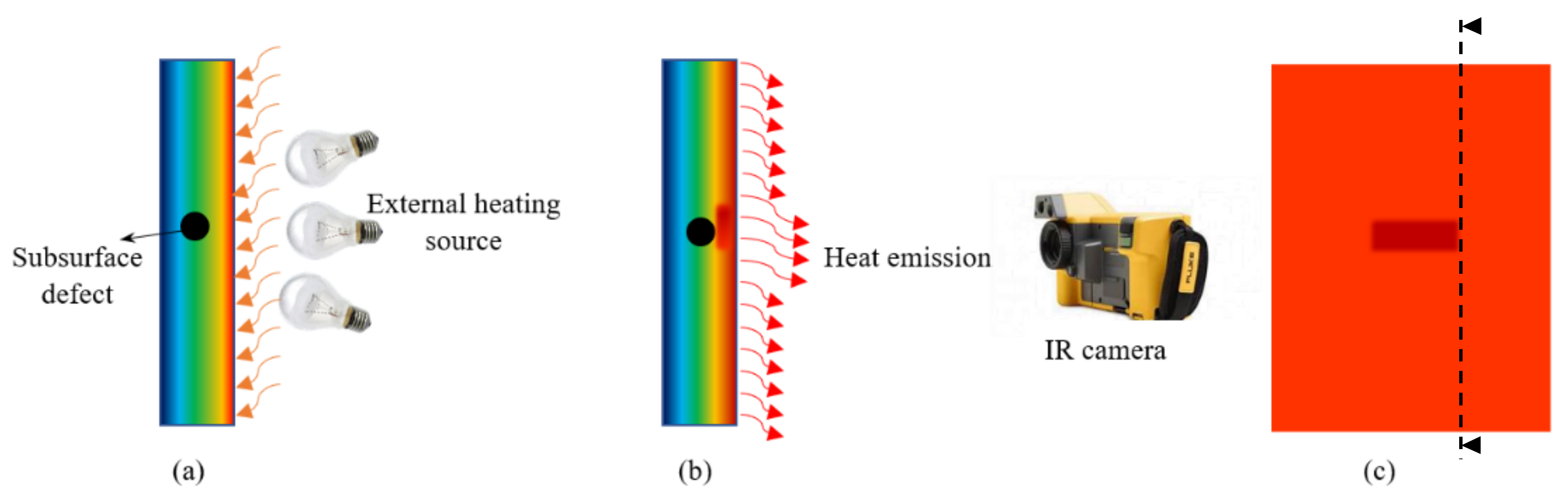
2.2. Infrared Thermography (IRT)

All objects (e.g., solid, liquid) emit infrared radiation in many wavelengths; however, each of these wavelengths correspond to a specific temperature [18]. Infrared thermography (IRT) is an NDE technique that employs an infrared (IR) camera to capture the infrared radiation that is emitted from a given surface, transforming it into electrical signals equivalent to the surfaces temperature profile. These signals are displayed in the form of a colorful thermal image known as a thermogram in which each color corresponds to a temperature according to the defined scale [18,19]. IRT is a popular NDE technique known for its portability, affordability, ease of use, large area of inspection, and ability to locate a range of surface and subsurface defects. IRT is effective at detecting the presence of any material with a different thermal conductivity, such as an air- or a water-filled defect in a homogeneous solid. In the presence of a thermal gradient through the thickness of the investigated object, the IR image will identify these anomalies, provided that the thermal conductivity is different, as shown in Figure 1. The thermal gradient needed for IRT can be generated through passive or active methods. In passive IRT, the ambient environment and sunlight are used to generate this thermal gradient [20]. In active IRT, an external heat source is used to provide the necessary energy to induce the thermal gradient [20]. The imposed thermal gradient can be generated from the same side as the measurement, known as the reflection method, to locate superficial anomalies, or from the opposite side of the measurement, which is known as the transmission method, to identify deep anomalies [18]. The transmission method is useful when both sides of the object under study are accessible. However, since ASTs are kept full or half-full all year, only the outside of the tank is accessible for imposing heat. Therefore, this research primarily focuses on the reflection method.
When considering active thermography, different heating sources can be considered, such as laser heating, halogen lamps, flash lamps, ultrasonic excitation, microwaves, etc. [21]. However, one of the challenges in using IRT on tanks constructed from HDPE is the material’s low thermal diffusivity (≈1.80 × 10⁻⁷ m2/s [22]). This means that it takes a lot of energy to manipulate the HDPE material’s temperature and initiate heat transfer over the thickness of the object. Regardless, a number of studies have demonstrated the effectiveness of IRT for polyethylene components, such as pipes [23,24,25], pipe joints [26,27,28], and composites [29]. To accommodate the low thermal diffusivity, six 500-watt halogen lamps with a total power of 3000 watts at a distance of 0.4 m were used to heat up the object for three minutes. This power and heating time were determined through a set of trial and error experiments and include a consideration of the practical aspects of the test’s utility in the field for evaluating the real ASTs. Concentrating the heating power on a small region, over a short distance (0.4 m), and with a three-minute duration, offers enough of a temperature gradient over the thickness of the specimen to be inspected, at least for this study. This way, more excitation power can be delivered in a shorter period of time, resulting in more effective heating.
For this research, a Fluke TiX580 thermal imager (IR camera), with the features shown in Table 1, was used. In this research the goal of using an IR camera was to detect subsurface anomalies and not for accurate temperature measurements. Since the appearance of the defects depends on the existing thermal gradient across the object’s thickness and since the object temperature (OT) was not controlled, the IR camera’s temperature range was narrowed manually and set to the range [O.T-5 °C, O.T + 10 °C]. The reasons for this were: (1) to reduce the time needed for defects to appear in the thermal images and (2) to detect anomalies with the highest contrast. The other settings of the IR camera can be found in Table 2.
In this study, the most effective empirical procedure was determined to be as follows: (1) the IR camera was positioned 1.5 m away from the object, (2) the target object was heated by the external heating source for three minutes, and (3) immediately after removing the heating source, the change in temperature of the object during the cooling phase was monitored for three minutes (capturing images every 10 s). The distance between the camera and the object was defined by a preliminary investigation that studied the correlation between the distance and the area under study and the smallest observable defect size at the best condition. For this purpose, some partial-depth holes with different diameters were created on a HDPE plate, and then the defects were exposed in a way such that they faced the heating source and IR camera. This is the best condition in which all of the defects could be observed without concerning the low thermal diffusivity of HDPE and thermal attenuation during the experiment. The IR camera was set at different distances and the data were plotted as shown in Figure 2. As can be seen in Figure 2, a distance of 1.5 m is the greatest distance before the minimum observable defect size increases by about 1 mm. Since this research was trying to study the feasibility of using IRT technique on real ASTs and for the field investigation, the thermal images have been reported without any additional image processing.

2.3. Ultrasonic Testing (UT)

The IRT technique with the reflection method described previously helps to identify the existence of superficial subsurface defects with their approximate size and location. However, this technique cannot give information about the depth of the defect or the location of the abnormality over the thickness of the object and if there are several stacked defects on the same spot. Therefore, after the potential abnormal areas were identified by IRT, a more detailed investigation is needed. In this research both conventional pulse-echo ultrasonic testing (PEUT) and phased array ultrasonic testing (PAUT) have been considered since both of these tests need access to only one side of the specimen under investigation and allow for the inspection of ASTs that are filled with liquid.
PEUT, also known as pulse reflection ultrasound, is a conventional one-sided UT in which a single transducer generates an ultrasonic pulsed wave from one side of a specimen into the specimen. That same probe then receives a response signal that has been reflected by an inhomogeneity, such as a defect, or the back wall of the specimen [30]. PAUT probes are composed of multiple ultrasonic elements that act as a synthetic aperture to “sweep” its focus without moving the probe [31,32], thereby providing significantly more versatility and range than conventional methods. Since the probe’s focus is “swept,” even defects that are stacked can be detected, which would not be possible by conventional pulse-echo methods [33]. PAUT has shown great capabilities to detect the embedded defects in HDPE pipes and joints [34,35,36,37,38,39,40,41,42].
By calibrating the measuring equipment to the P-wave velocity of the AST material with knowledge of the wall thickness, both PEUT and PAUT can locate hidden abnormalities. One disadvantage for application of UT to HDPE is the potential for significant acoustic attenuation and dispersion due to the viscoelasticity of HDPE, with energy losses reported at 18 dB/inch (7 dB/cm) and as large as 38 dB/inch (15 dB/cm) [33,34,43]. Therefore, based on the AST wall thickness and defect sizes, a range of ultrasonic frequencies needs to be considered; for instance, while higher frequencies will likely yield better resolution, the signal will diminish due to increased scattering [44]. Another challenge with PEUT is that when the defect size is smaller than the probe size, waves will propagate through both the irregularly damaged area and intact area; therefore, more peaks will appear in the response signals, making it difficult to identify the correct peak for the defect in order to characterize its geometry and its location over the thickness.
In this research, a Proceq Flaw Detector 100 ultrasonic instrument was used in combination with a 5 MHz mono probe from Sonatest for PEUT tests and a phased array water wedge probe from SensorScan with 2.25 MHz for PAUT tests. Water wedges have been used in other studies of HDPE material [37,38,39], primarily because the relatively slow acoustic velocity of HDPE would result in a negative refraction from other commonly used PAUT wedge materials. Wave velocity calibration was done with the mono probe before starting each measurement. The settings used for the calibration is summarized in Table 3.
For viscoelastic materials, such as HDPE at the temperatures studied here, the attenuation coefficient and phase velocity will vary with temperature [45,46]. Therefore, since the AST temperature will vary seasonally, the effect of temperature on wave velocity was evaluated. For this purpose, Echo Pure low viscosity couplant from Echo Ultrasonics LLC was used to investigate the wave velocity change vs. temperature on HDPE plates with thicknesses of 12.7 mm and 19.05 mm. The results in Figure 3 show that the thickness of the specimen does not impact the sound wave velocity measurement. Results in Figure 3 show that when the temperature decreases, the sound wave velocity increases. The reason is that in colder temperatures, HDPE becomes denser in structure due to the change of crystallinity and amorphousness of hydrocarbon chains and due to the change in the degree of crosslinking and branching [47,48,49]; therefore, the sound wave travels faster through the denser material at colder temperatures. These results demonstrate the importance of measuring the wave velocity in the field before inspecting ASTs.
To study the impact of the utilized couplant on the measured sound wave velocity, the experiment was repeated with four variations of couplants while testing a 12.7 mm thick HDPE. The couplants used for this preliminary investigation were water, petroleum jelly, Echo Pure low viscosity, and Echo Pure 414 FL. The results in Figure 4 show that there is little to no effect of couplant type on wave velocity, at least for the couplants examined here.
The other concern about UT on the HDPE plate for the field tank evaluation is the impact of UV degradation. Since the HDPE tested in Figure 3 and Figure 4 was new, the temperature dependence was also evaluated for 15-year-old weathered HDPE collected from a failed AST to explore the potential field variability. The weathered HDPE, shown in Figure 5 exhibited significant shallow cracking on the interior of the tank. Figure 6 compares the temperature difference between the new and weathered HDPE, which demonstrates that most of the measured data placed in the 95% prediction interval. These observations imply that weathering does not appear to considerably affect the sound wave velocity.

2.4. Specimen Preparation

While the eventual objective of this project is to develop recommendations for field investigation of ASTs, the present study focused on a laboratory study so that additional variables could be controlled. In the field, the ASTs experience different thermal gradients on the sun-facing vs. shade-facing sides of the tank as well as variability in the gradients as a function of brine solution temperature and how full the tank is. Therefore, in order to better control some variables, a small-scale water tank was created in the laboratory with interchangeable plates of varying thickness and defect content. Figure 7 shows the 610 mm × 610 mm × 304.8 mm (24 in. × 24 in. × 12 in.) tank used for this purpose. One side of the tank was removed, allowing for HDPE plates of thicknesses 12.7 mm (0.5 in.) and 19.05 mm (0.75 in.) to be installed for experiments. These plate thicknesses were selected as representative of in-service ASTs. These plates had specific manufactured defects to allow for calibration of the IRT and UT methods; the defect map and defect sizes created on the plates with the thicknesses of 12.7 mm and 19.05 mm are shown in Figure 8 and Table 4.
For each plate installed on the water tank, the IRT experiment was repeated 20 times on different days under different environmental conditions to get a wide range of temperature differences between the water and tank exterior. The condition information for each measurement is summarized in Figure 9. There were some parameters impacting the measurements, such as the specimen size, impact of water temperature in the tank, and relative humidity (RH%). In order to study the impact of specimen size on the heat transfer properties, a preliminary study was completed by applying the IRT technique on two plates with dimensions 304.8 mm × 304.8 mm × 12.7 mm (12 in. × 12 in. × 0.5 in.) and 610 mm × 610 mm × 12.7 mm (24 in. × 24 in. × 0.5 in.). Both plates were heated for ten minutes. The temperature change of the center of both plates was recorded and plotted. To study the impact of water and its temperature on the measurements, the water temperature was changed manually via a water heater. This approach simulates the water and tank temperature differences occurring over a day from 12:00 AM to 11:59 PM in a real AST. Since the IRT experiments in this study were completed outside the lab, there was no control over the RH%; therefore, the impact of RH% on the measurement is not the focus of this study.

3. Results and Discussion

3.1. Survey

Seventeen states responded to the questionnaire. Nearly 5100 ASTs are in service in those 17 states that responded to the questionnaire. The tank capacities vary from 3785 L to 75,708 L (1000 gallons to 20,000 gallons), but the most typical capacities are in the range of 18,927 L to 41,640 L (5000 gallons to 11,000 gallons). More than 65% of the all tanks in service have an age between 5 and 14 years. Of the states surveyed, 92% are using polyethylene tanks to store their deicing salt solutions. The rest are using fiberglass and plastic tanks. The state DOTs reported that the thickness of their ASTs have been designed for 1.7 to 1.9 times the specific gravity of the solution and reported different values between 12.7 mm (0.5 in.) and 19.1 mm (0.75 in.) for the wall thickness. Seven states reported at least one tank failure experience, two of which were fitting failures. The remainder were due to an unexpected complete rupture of the tank. Maryland DOT reported two complete failures that were like an explosion. These findings further indicate the importance of using NDT to evaluate the ASTs condition to prevent a catastrophic failure. state DOTs currently do not have specific criteria to match the condition of the tanks under their control with criteria that would indicate a given tank needs to be removed from service. For this reason, they try to remove tanks from service before they reach an age of 12 to 15 years. This demonstrates an area for research to develop a series of test methods and guideline for determining when to remove a tank from service. Moreover, there are no specific guidelines for state DOTs to follow to assess the condition of the tanks under their control. For this reason, most of DOTs simply conduct a monthly visual inspection by walking around the tanks. Seven DOTs reported issues with fittings during their visual inspections. In most cases, the state DOTs keep their tanks full year-round. This common practice shows the importance of using new NDTs that need access to only the outer side of the tank. Except for the Oregon DOT, who unsuccessfully attempted to patch one of their tanks, no other repairs (except fixing the leakage in fittings) were reported the respondents.

3.2. IRT

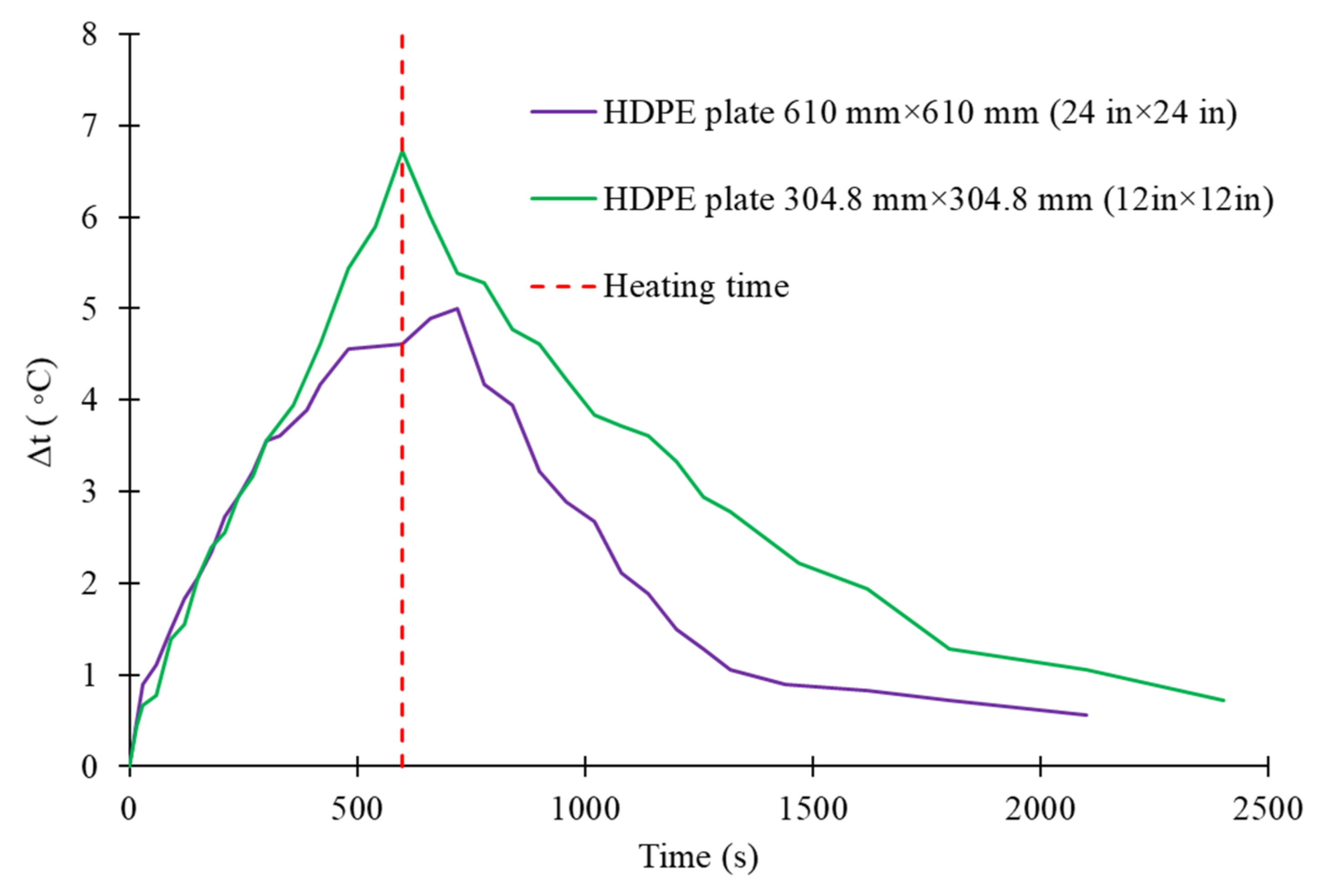
3.2.1. Impact of Specimen Dimension on Heat Transfer

Two HDPE plates with different sizes were selected to study the impact of specimen size on the IRT measurements. The smaller plate with dimensions of 304.8 mm × 304.8 mm × 12.7 mm (12 in. × 12 in. × 0.5 in.) was chosen to allow the whole area to be heated by the external heating source during the IRT. A larger sample with dimensions of 610 mm × 610 mm × 12.7 mm (24 in. × 24 in. × 0.5 in.) was chosen to ensure only the center area was impacted by the applied heat. The results of the IRT technique on both HDPE plates are shown in Figure 10. The vertical axis shows the temperature difference between the center of the HDPE plates at different times and the initial temperature before starting the experiment. Results demonstrate that when the dimension of the specimen increases, the heat propagates towards the cold areas to induce a uniform temperature between the heated area and the surrounding area. For this reason, the maximum temperature difference is lower in the plate with larger dimensions compared to the smaller plate with which the entire area is impacted by heating. This shows that, when the specimen size increases, more energy (i.e., power and time of heating) is required to manipulate the temperature of the HDPE and induce the same thermal gradient over the thickness of the specimen. When the specimen size is small, the whole area is heated up and the heat transfers only through the thickness of the sample. However, when the size of the specimen increases, the heat transfers in all directions of the HDPE plate and through the thickness of the sample. Therefore, it may reduce the efficiency of IRT in the field. This shows that, in order to apply IRT to the evaluation of HDPE ASTs in the field, a series of field tests are required to prove the efficacy of this technique. This shall be studied in future work.

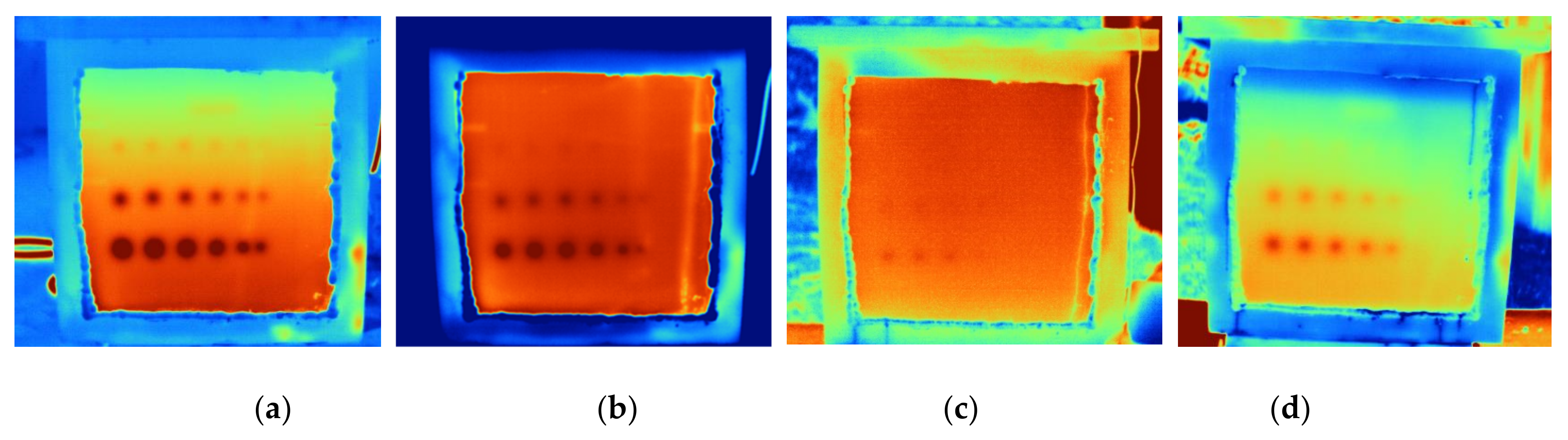
3.2.2. Defect Detection with Active IRT on HDPE

At first, to investigate the capability of the IRT technique to detect abnormalities, the experiment was performed with an empty water tank. The empty tank was chosen because both sides of the HDPE plate had the same temperature and there was no initial thermal gradient present across the plate thickness. Figure 11 shows that IRT has the potential to detect some of the abnormalities that exist in the HDPE. Figure 11 indicates that, when there is no initial thermal gradient over the thickness (t), only anomalies that are shallow and are located less than 0.5 × t from the outer surface can be detected. For this reason, when there was no initial thermal gradient, S.H.1, S.H.2, SH.4, R3, and R2 were observed. This happened due to the low heat diffusivity of HDPE and high heat attenuation. For this reason, not enough heat is transferred to the other side of the plate over deep defects (like scratches, and R1) to create a contrast on the thermograms. The minimum defect size that could be detected for shallower defects (i.e., R3 defects) was a circular defect with a diameter of 5 mm. This observation shows that under this circumstance, defects with a size of 2.8 mm and smaller do not impact the heat transfer and therefore cannot be observed by IRT. Moreover, as shown in Figure 11, all of the defects that could be observed by IRT with no initial thermal gradient prior to heating appear during the first 30 s after removing the heating source. When the tank is filled with water, the water temperature on the other side of the plate can induce an initial thermal gradient over the thickness, which can impact the observation. Therefore, the study was completed on the full tank under different circumstances such as different initial thermal gradient or different water temperatures.
The quantitative results of IRT on both plates (thicknesses of 12.7 mm and 19.05 mm) tested under different circumstances are shown in Table 5 and Table 6. In these tables, the initial thermal gradient is the temperature difference between the exterior and interior surfaces of the tank wall (ΔT = Tsurf – Tint) before starting the experiment and applying the external heat. Tint is equal to the water temperature when the tank is full. Negative values for ΔT imply that the water temperature inside the tank had a higher temperature than the outer surface of the tank. If the tank was empty, it was assumed that the exterior and interior surfaces of the tank wall had the same temperature, and therefore the initial thermal gradient was equal to zero.
For the side holes, the minimum defect size that could be detected by IRT was recorded as the diameter of the hole. The parameter δtapp represents the temperature difference on the surface between the cooling phase, when the defect appeared on the thermogram, and the initial surface temperature before starting the experiment. The parameter tapp represents the time after removing the heating source when the defect first appeared on the thermogram. δtdis represents the surface temperature difference between when the defect disappeared on the thermogram and the initial temperature before starting the experiment. The tdis represents the time after removing the heating source when the defect disappeared on the thermogram. For the measurements in which the detected defect was visible throughout the cooling phase and time of measurement (t = 180 s), it was assumed that the defect disappeared when the thermal gradient was diminished (δtdis = 0) in about 7 h (tdis = 10,000s).
By comparing the results in Table 5 and Table 6, it is readily seen that, for the HDPE plate with a thickness of 12.7 mm, it takes a longer time to detect defects compared to the HDPE plate with a thickness of 19.05 mm. The reason for this is that heating the plate with a thickness of 12.7 mm for three minutes caused it to saturate the thermograms and therefore more time was required to obtain unsaturated images with observable defects. Because of this heat saturation in the measurements on the 12.7 mm thick HDPE, all of the detected defects did not disappear until the end of the experiment. This means that for the HDPE plate with the thickness of 12.7 mm, a lower heating power or a shorter heating time can be used for faster anomaly detection. While investigation of the impact of RH on these measurements was not the goal of this study, results show that when the RH decreases, the minimum observable defect size decreases. This observation can be attributed to two reasons: (1) a lower RH results in more efficient heat transfer, allowing the surface to receive more heat compared to when the RH is high and moisture between the heating source and object attenuates some portion of the heat energy, and (2) when the RH is low, dispersion of the emitted IR signature from the object is reduced, which results in more accurate measurements.
In the experiments shown in Table 5 and Table 6, 2.8 mm was the minimum interior defect size that could be observed in the thermograms if it was located at 0.25t. However, looking at the norm shows that 5 mm can be conservatively considered as the minimum defect size that could be detected. If the interior defect was located on about 0.5t, the minimum defect detection size that could be detected was 7.0 mm. The minimum size of the side hole that could be detected was 3.175 mm.
As determined from the data in Table 6, when the tank was full of water, the observed interior defects remained observable until the end of the experiment for most measurements, while the side holes defects disappeared before the experiment was finished. When the tank was empty, the side holes were observable in the thermograms for most of the measurements until the end of the experiment. Moreover, when the tank was full, the interior defects appeared as cooler spots, and the side holes appeared as hotter spots compared to the intact areas, while when the tank was empty, all of the interior and side holes looked hotter than the intact areas. These last two statements imply that water inside the tank alters heat transfer. More investigation of the results of the impact of water temperature on heat transfer shows that as the water temperature inside the tank increases, the minimum observable defect size increases. The reason for this is that when the temperature of the water is greater than the tank exterior (ΔT < 0), most of the heat energy is consumed to increase the surface temperature to reach the water temperature and induce zero thermal gradient (ΔT = 0). After that, the rest of the energy is used to induce a positive thermal gradient. Therefore, the induced thermal gradient decreases as the water temperature increases. More details are provided in Section 3.2.3. For Experiment #9 in Table 6, no external heating source was used because three minutes of heating was not enough to induce a positive thermal gradient for defect detection during the cooling phase. Therefore, this measurement along with measurements 15 and 20 was used for the investigation of transmission IRT.
Results in Table 5 and Table 6 show that scratches inside the tank, very small subsurface defects (in this study S.H.3 with the diameter size of 1.6 mm), and deep defects (R1 interior defects) cannot be observed. The reason for this is that the HDPE has a very low thermal conductivity, thermal diffusion, and high heat attenuation characteristics. Therefore, the induced thermal gradient generated by three minutes of heating with 6000 watts of power may not be sufficient to reach these deep anomalies. Tiny subsurface anomalies such as defect S.H.3 in this study do not interfere with the heat transfer. Therefore, the emitted IR from the tiny subsurface defects is not much different from that in the intact areas, making detection by IRT difficult. In general, in this study, the defects that were located less than half the thickness of the tank wall (0.5t) from the external surface could be detect by IRT.

3.2.3. Impact of Water Temperature on Defect Detection in Active IRT

The results shown in Figure 12 indicate that the water inside the tank can impact both the time of appearance of each defect in the thermograms and the minimum observable defect size. When the tank is empty, both sides of the tank wall have almost the same temperature (ΔT = 0). Therefore, all of the heating energy applied on the outside of the wall will be transferred through the wall thickness and induce a thermal gradient.
In Figure 12b, when the tank is filled with water with almost the same temperature of the tank exterior (ΔT ≈ 0), the induced thermal gradient increases; the reason for this is that water has a high thermal capacity and needs more energy to increase the temperature. On the other hand, the water and the interior side of the tank are in equilibrium. Therefore, when the applied heat reaches the other side of the tank, the interaction between the water and the interior wall of the tank causes a smaller temperature change in comparison to the time in which the tank is empty. In Figure 12c, when the water has a lower temperature than the tank exterior, it creates the maximum thermal gradient across the thickness.
In Figure 12d, the water inside the tank has a higher temperature than the tank exterior. In this case, when heat is applied on the surface, the temperature of the tank exterior increases first to reach the temperature of the interior side and then increases past the interior temperature; this means that the thermal gradient induced on the thickness with the same amount of energy is negligible.
Another observation made was that the water temperature impacts the initial ΔT. A higher positive initial ΔT results in shorter time of defect appearance in the thermograms. In Figure 12 if the time t = 0 is to be used for comparison, then it can be seen that, when the ΔT increases from Figure 12a–c, the time for observing the defects becomes shorter. In Figure 12c, which shows the highest ΔT, most of the deep defects were observed immediately after removing the heating source. However, as shown in Figure 12d, where ∆T is a negative value, even after 400 s, no defect was observed. As shown in Figure 12a, the minimum defect size in R2 was an interior defect with a diameter of 7.0 mm, and in the R3 defect series, the minimum observable defect size was 5 mm in diameter. When the ΔT increased, as seen in Figure 12b, the minimum defect size in the R2 defect series was an interior defect with a diameter of 10.0 mm, and in the R3 defect series the minimum observable defect size was 5 mm in diameter. Therefore, the water temperature impacts both the minimum detectable defect size and the time for the appearance of defects on the thermograms.

3.2.4. Indirect Transmission IRT
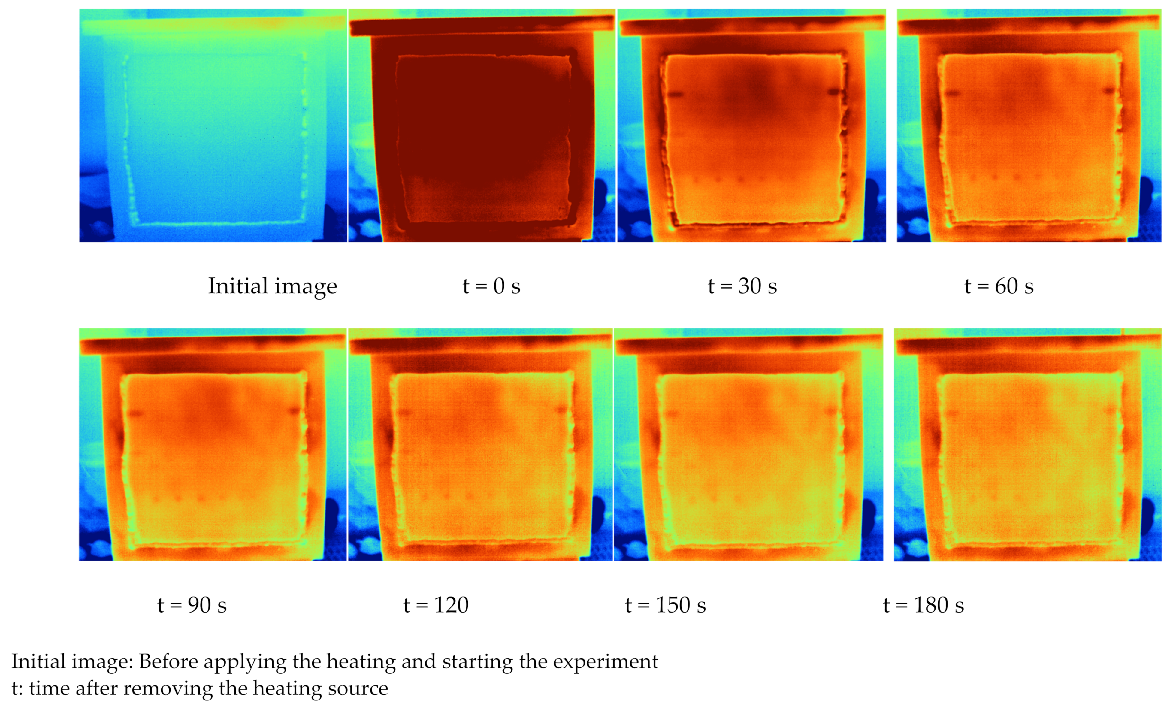
The initial images of Experiments #9, #15, and #20 in Table 6 were used to indirectly study transmission IRT. In these three experiments, the water inside the tank had a higher temperature than the outer side of the tank, and therefore water could be used as a heating source on the opposite side of the wall, which is required for transmission IRT. For this reason, the initial images before applying an external heating source were used. Figure 13 shows that transmission IRT can help to detect many anomalies in a very short period of time without applying external heating and spending additional time monitoring the defect appearance during the cooling phase. These defects that were observable and appeared at the same time on the first thermogram. The smallest interior defect that could be observed was the defect 5 mm in diameter when the tank was filled with 45 °C water and when the wall temperature did not reach equilibrium with the water (Figure 13a,b). Figure 13a shows that, when the water and the interior side of the tank wall did not reach a temperature equilibrium and had the highest absolute thermal gradient over the wall thickness, deep defects such as scratches and R1 defects could be detected. For cases when the interior tank wall and water reached a temperature equilibrium (Figure 13c,d), the smallest observable defect size increased to 7.0 mm and the deep defects such as R1 and subsurface defects like S.H.4 could not be detected properly.
Experiment #9 could not be extended for 24 h to allow the water and interior side of the tank wall to reach equilibrium. This was because the water heater that was used to keep the water temperature constant was not capable of maintaining a 45 °C temperature. In general, it can be concluded that transmission IRT helps to detect the shallow anomalies with less energy in a shorter time. Transmission IRT can be applied in the field if the best time frame is found in which the brine in the tank is a higher temperature than the outer side of the tank. This is in the scope of future work.
Figure 13d shows that if there is leakage (at the bottom of the tank in the figure), it can be detected immediately by using the IR camera without applying any heating. This helps to rapidly evaluate the ASTs for leakage and locate the origin of the leakage.

3.2.5. Passive IRT

In passive IRT, represented in Experiment #19 in Table 6, cold water with temperature of 9.8˚C was used to produce a positive ΔT due to the ambient temperature. The passive thermography worked in this measurement because the cold water inside the tank induced a very high positive initial thermal gradient (ΔT = 8.42 °C) over the thickness of the HDPE plate. Therefore, the ambient temperature could act as the external heating source, allowing shallow defects (R2 and R3) as well as subsurface defects (S.H.1, S.H.2, and S.H.4) to be detected as shown in Figure 14 The result provided in Figure 14 shows that passive IRT has the potential to detect these shallow defects; however, the optimum ΔT for passive thermography is still unknown. This is the subject of future work.

3.3. Ultrasonic Testing (UT)

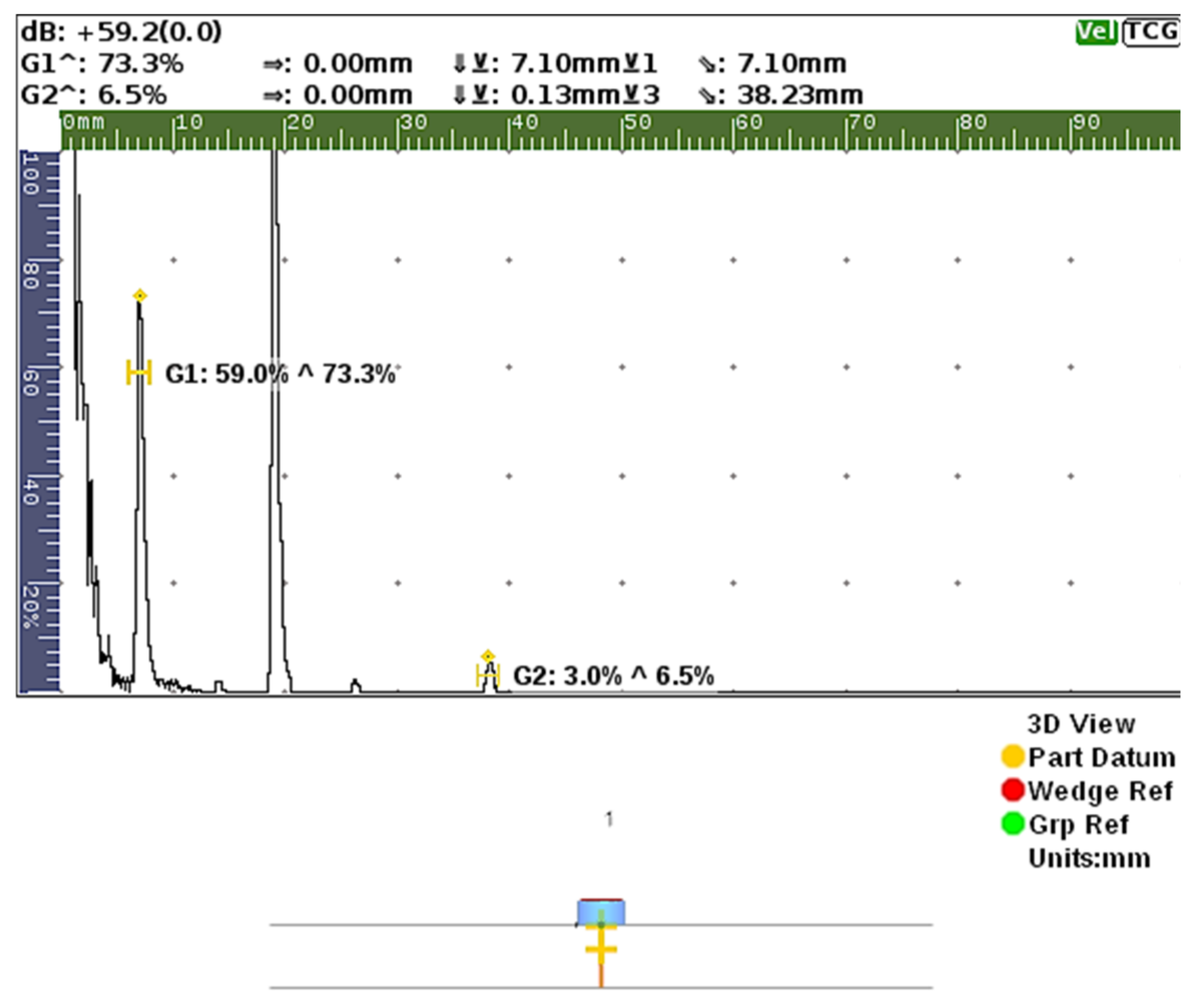
3.3.1. Pulse-Echo Ultrasonic Testing (PEUT)

Ultrasonic testing could indicate subsurface defects and useful information on the general location of these defects.
Figure 15 shows the results of pulse-echo ultrasonic testing (PEUT) for detecting a single interior defect (i.e., the R2 defect on the HDPE plate with a thickness of 19.05 mm). By positioning the first cursor on the right peak, the depth of the defect from the surface could be measured. To be more specific, by positioning the cursors on the right peaks and by subtracting “G2↓v” from “G1↓v”, the location of the defect could be characterized. Additionally, the location of the defect can be seen in the bottom window in Figure 15.
The experiment was repeated on a subsurface defect (i.e., S.H.2 on the 19.05 mm thick plate). As shown in Figure 16, there are three peaks. Two peaks are attributed to both sides of the plate, and the other peak (first peak from the left) is attributed to the subsurface hole. Therefore, by positioning the cursors on the peak correlated to the hole and the peak of surface of the plate, the location of the subsurface defect can be characterized as shown in Figure 16. If the defect is smaller than the probe size, or the probe is located on the border of the defect and flawless area, more peaks will be observed in the response signals as shown in Figure 17. This makes the interpretation of PEUT results difficult.
PEUT was also performed on a plate with two and four stacked side hole defects, shown in Figure 18 and Figure 19 respectively. By comparing the last two figures, it can be seen that the results resemble each other. These results indicate that PEUT is unable to characterize these stacked defects.

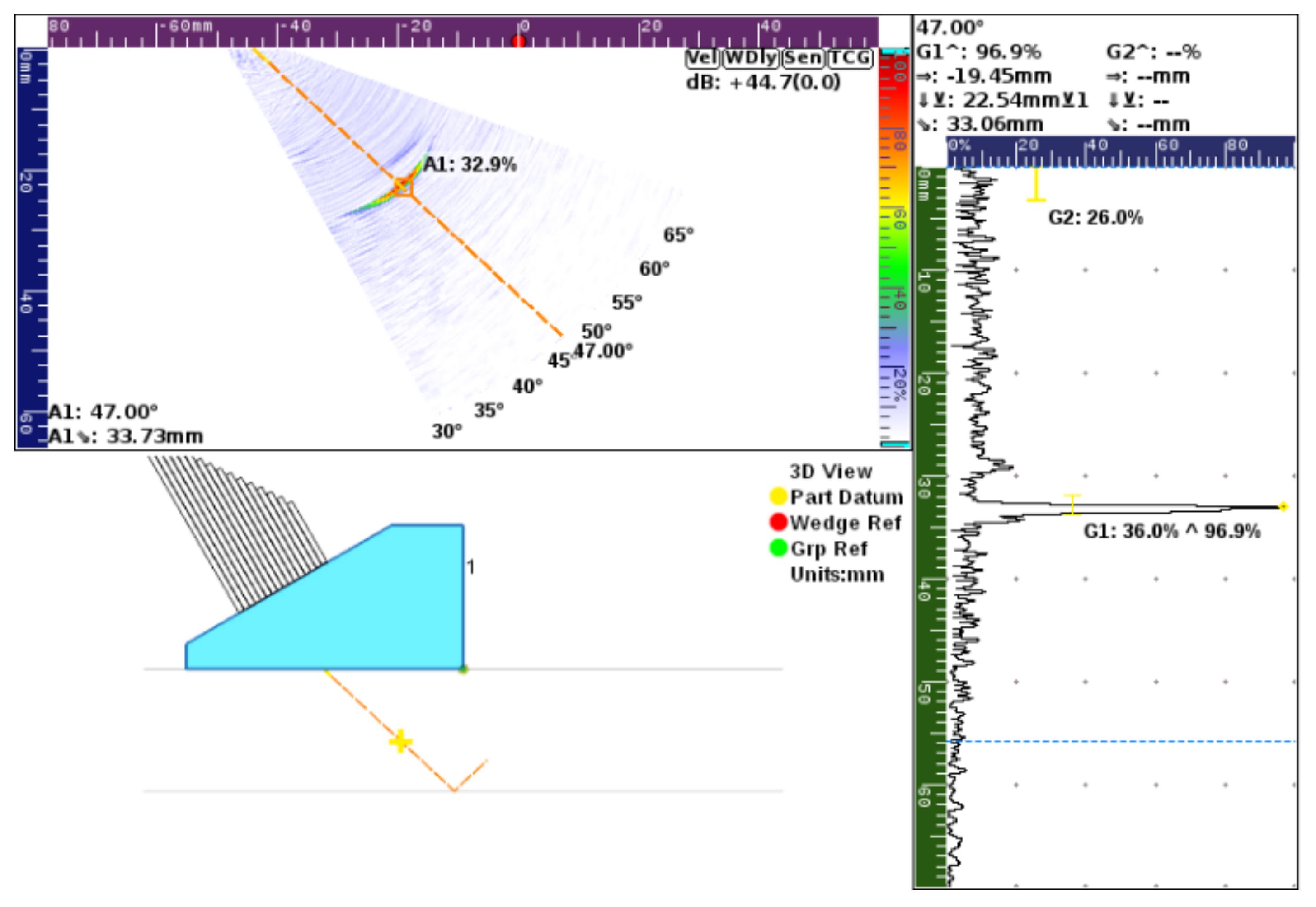
3.3.2. Phased Array Ultrasonic Testing (PAUT)

Phased array ultrasonic testing (PAUT) was used on a single interior defect (the biggest defect in R3), two stacked defects, and four stacked defects. The results are shown in Figure 20, Figure 21 and Figure 22. When there was an interior defect with dimensions bigger than the wedge, only a single defect was observable on the UT responses, as shown in Figure 20. However, if a defect with smaller size than the wedge existed, more peaks and defects were observed in the UT responses as shown in Figure 22.
The top window in Figure 21 shows two defects identified in the PAUT response. In addition, two peaks on the linear signals on the right side of the figure could be observed, which further proves the existence of the two defects. Depending on the positioning of the first and second cursors in the software, the depth of the defects from the surface or the distance between the defects can be measured. From the results shown in Figure 21, the distance between the stacked defects was measured in the top red box. Moreover, the width of the defects on the sectorial response shows the size of the defect. Figure 22 shows the results of PAUT on the 19.05 mm thick HDPE plate with four stacked defects. There are four defects on the sectorial PAUT response. In addition, the four peaks on the signals on the right side of the figure further prove the existence of the four defects. As was performed for the two stacked defects, the distance between the defects or the depth of those defects can be estimated by positioning the first and second cursors on the right peaks. Figure 21 and Figure 22 show that PAUT is a powerful technique that can characterize defects accurately. Moreover, while the results show that UT can be used as an effective technique to characterize defects, further work is needed to study its efficiency when used as a method of evaluating ASTs in the field. This is the subject of future work.

4. Conclusions

In this study, the feasibility of using two non-destructive test methods for evaluation of high-density polyethylene (HDPE) liquid storage tanks by both infrared thermography (IRT) and ultrasonic (UT) methods was studied. While reflection IRT was the focus of this work, transmission and passive IRT were explored as well. Both conventional pulse-echo ultrasonic testing (PEUT) and phased array ultrasonic testing (PAUT) have been considered since both of these tests need access to only one side of the specimen under investigation and allow for the inspection of storage tanks filled with liquid. In general, the following conclusions can be drawn from this study:
  • IRT has shown the potential to detect leakage and some subsurface abnormalities in HDPE plates.
  • IRT is useful for locating shallow subsurface defects that are located at less than half of the thickness of HDPE plates.
  • Water temperature can impact IRT measurements of an HDPE tank by influencing the minimum detectable defect size and time of appearance of the defects on the thermograms.
  • Transmission IRT helps to detect the shallow anomalies in HDPE water tanks with less energy in a shorter amount of time.
  • For HDPE with high thermal attenuation properties and very low thermal conductivity, the passive IRT works best when there is a very high positive initial thermal gradient over the thickness of the specimen.
  • UT is sensitive to both interior and subsurface abnormalities of HDPE plates.
  • UT is highly accurate in determining flaw position and estimating flaw size and shape in HDPE plates.
  • PAUT is a powerful technique that can help to detect and characterize multiple stacked defects in HDPE plates.
  • Ultrasonic testing can be used as a complement to IRT for a more detailed inspection of HDPE ASTs.

Supplementary Materials

The survey questionnaire is available online at https://0-www-mdpi-com.brum.beds.ac.uk/article/10.3390/civileng2040045/s1.

Author Contributions

Conceptualization, A.B. and A.S.B.; Methodology, A.B. and A.S.B.; Formal Analysis, A.B. and M.M.d.; Investigation, A.B. and M.M.d.; Data Curation, A.B. and M.M.d.; Writing—Original Draft Preparation, A.B. and M.M.d.; Writing—Review and Editing, A.B., M.M.d., and A.S.B.; Visualization, A.B. and M.M.d.; Supervision, A.S.B.; Project Administration, A.S.B.; Funding Acquisition, A.S.B. All authors have read and agreed to the published version of the manuscript.

Funding

This research was funded by Virginia Transportation Research Council (VTRC), Project 117955.

Data Availability Statement

The data presented in this study are available on request from the corresponding author.

Acknowledgments

The authors thank Amy A. O’Leary and Lewis Lloyd at VTRC for their help during survey and for providing necessary data. The authors would like to thank David Mokarem and Brett Farmer at Virginia Tech for their assistance during the preparation of specimens. The authors appreciate the support from Fred Whitford from Purdue University for providing a weathered piece of a failed brine storage tank. The authors would like to thank Echo Ultrasonics LLC for providing ultrasonic couplants to the researchers.

Conflicts of Interest

The authors declare no conflict of interest.

References

  1. Ketcham, S.; Minsk, L.D.; Blackburn, R.R.; Fleege, E.J. Manual of Practice for an Effective Anti-Icing Program: A Guide for Highway Winter Maintenance Personnel; Federal Highway Administration: Washington, DC, USA, 1996.
  2. Whitford, F.; Salomon, S.; Oltman, D.; Obermeyer, J.; Hawkins, S.; Pearson, M.; Overstreet, B.; Titus, M.; Lambert, S.; Hawkins, M. Poly Tanks for Farms and Businesses: Preventing Catastrophic Failures, Report PPP-77. 2008. Available online: https://www.extension.purdue.edu/extmedia/ppp/ppp-77.pdf (accessed on 13 August 2021).
  3. Cornell, J.R.; Baker, M.A. Catastrophic tank failures: Highlights of Past Failures along with Proactive Tanks Designs. In Proceedings of the US EPA Fourth Biennial Freshwater Spills Symposium (FSS 2002) Sheraton Cleveland City Centre Hotel, Cleveland, OH, USA, 19–21 March 2002. [Google Scholar]
  4. Abell, D.H. A Study of the Cause of Failure of Rotationally Molded, High-Density Polyethylene, Sodium Hypochlorite Storage Tanks, Brigham Young University. 2011. Available online: http://hdl.lib.byu.edu/1877/etd4342 (accessed on 13 August 2021).
  5. Whitford, F.; Hawkins, S.; Holland, L.; Carr, B.; Meredith, D.; Ileleji, K.; Campbell, D.; Gentry, L.; Hamby, L.; Roach, M.; et al. Aboveground Petroleum Tanks: A Pictoral Guide, Report PPP-73. 2007. Available online: https://www.extension.purdue.edu/extmedia/PPP/PPP-73.pdf (accessed on 13 August 2021).
  6. Myers, P.E. Aboveground Storage Tanks; McGraw-Hill Education: New York, NY, USA, 1997. [Google Scholar]
  7. Atherton, W.; Ash, J.W. Review of Failures, Causes & Consequences in the Bulk Storage Industry. 2007. Available online: https://citeseerx.ist.psu.edu/viewdoc/download?doi=10.1.1.489.7637&rep=rep1&type=pdf (accessed on 28 September 2021).
  8. U.S. Chemical Safety and Hazard Investigation Board, Allied Terminals, Inc. Catastrophic Tank Collapse, Report 2009-03-I-VA; U.S. Chemical Safety Board: Washington, DC, USA, 2009.
  9. United States Environmental Protection Agency. Office of Solid Waste and Emergency Response, Rupture Hazard from Liquid Storage Tanks, EPA 550-F-09-004; United States Environmental Protection Agency: Washington, DC, USA, 2009.
  10. Carrasco, F.; Saurina, J.; Colom, X. FTIR and DSC study of HDPE structural changes and mechanical properties variation when exposed to weathering aging during Canadian winter. J. Appl. Polym. Sci. 1996, 60, 153–159. [Google Scholar] [CrossRef]
  11. Hsueh, H.-C.; Kim, J.H.; Orski, S.; Fairbrother, A.; Jacobs, D.; Perry, L.; Hunston, D.; White, C.; Sung, L. Micro and macroscopic mechanical behaviors of high-density polyethylene under UV irradiation and temperature. Polym. Degrad. Stab. 2020, 174, 109098. [Google Scholar] [CrossRef]
  12. Mohan, B.C.; Jeyasekhar, M.C. Combination of infrared thermography and computed radiography nondestructive methods detect oil and gas storage tank drainage pipe blockage. In Proceedings of the 3rd Singapore International Non-destructive Testing Conference and Exhibition, Singapore, 4–5 December 2019; p. 8. [Google Scholar]
  13. Nisbet, R.T.; Pesce, M.D. NDT of welded steel tanks. NDT Tech. 2011, 10, 1–4. [Google Scholar]
  14. Kalra, L.P.; Shen, W.; Gu, J. A wall climbing robotic system for non destructive inspection of above ground tanks. In Proceedings of the 2006 Canadian Conference on Electrical and Computer Engineering, Ottawa, ON, Canada, 7–10 May 2006; p. 9376469. [Google Scholar] [CrossRef]
  15. Blakeley, B.; Emmanouilidis, C.; Hrissagis, K. Above-ground storage tank inspection using the ‘Robot Inspector’. Insight Non-Destructive Test. Cond. Monit. 2005, 47, 705–708. [Google Scholar] [CrossRef]
  16. Lowe, P.S.; Duan, W.; Kanfoud, J.; Gan, T.-H. Structural Health Monitoring of Above-Ground Storage Tank Floors by Ultrasonic Guided Wave Excitation on the Tank Wall. Sensors 2017, 17, 2542. [Google Scholar] [CrossRef] [Green Version]
  17. Spicer, M.; Hagglund, F.; Troughton, M. Development and validation of an automated ultrasonic system for the non-destructive evaluation of welded joints in thermoplastic storage tanks. In Proceedings of the 11th European Conference on Non-Destructive Testing, Prague, Czech Republic, 6–11 October 2014. [Google Scholar]
  18. Lourenço, T.; Matias, L.; Faria, P. Anomalies detection in adhesive wall tiling systems by infrared thermography. Constr. Build. Mater. 2017, 148, 419–428. [Google Scholar] [CrossRef]
  19. Barreira, E.; de Freitas, V.P. Evaluation of building materials using infrared thermography. Constr. Build. Mater. 2007, 21, 218–224. [Google Scholar] [CrossRef]
  20. Lagüela, S.; Díaz-Vilariño, L.; Roca, D. Infrared thermography: Fundamentals and applications. In Non-Destructive Techniques for the Evaluation of Structures and Infrastructure; Riveiro, B., Solla, M., Eds.; CRC Press: Boca Raton, FL, USA, 2016; pp. 113–138. [Google Scholar] [CrossRef]
  21. Verspeek, S.; Peeters, J.; Ribbens, B.; Steenackers, G. Excitation Source Optimisation for Active Thermography. Proceedings 2018, 2, 439. [Google Scholar] [CrossRef] [Green Version]
  22. Li, X.; Tabil, L.G.; Oguocha, I.N.; Panigrahi, S. Thermal diffusivity, thermal conductivity, and specific heat of flax fiber–HDPE biocomposites at processing temperatures. Compos. Sci. Technol. 2008, 68, 1753–1758. [Google Scholar] [CrossRef]
  23. Zhu, B.; Qiu, X.; Zhong, S.C.; Bin Fu, X.; Yang, X.X. Active Infrared Thermography for Defect Detection of Polyethylene Pipes. Adv. Mater. Res. 2014, 1044–1045, 700–703. [Google Scholar] [CrossRef]
  24. Murariu, A.C.; Lozanović-Šajić, J.V. Temperature and heat effects on polyethylene behaviour in the presence of imperfections. Therm. Sci. 2016, 20, 1703–1712. [Google Scholar] [CrossRef] [Green Version]
  25. Murariu, A.C.; Bîrdeanu, A.-V.; Cojocaru, R.; Safta, V.I.; Dehelean, D.; Boţilă, L.; Ciucă, C. Application of Thermography in Materials Science and Engineering. In Infrared Thermogr; Prakash, R.V., Ed.; InTech: London, UK, 2012; pp. 27–52. [Google Scholar]
  26. Omar, M.A.; Zhou, Y.; Parvataneni, R.; Planting, E. Calibrated Pulse-Thermography Procedure for Inspecting HDPE. Res. Lett. Mater. Sci. 2008, 2008, 186427. [Google Scholar] [CrossRef] [Green Version]
  27. Azad, M.J.; Tavallali, M.S. A novel computational supplement to an IR-thermography based non-destructive test of electrofusion polyethylene joints. Infrared Phys. Technol. 2018, 96, 30–38. [Google Scholar] [CrossRef]
  28. Doaei, M.; Tavallali, M.S. Intelligent screening of electrofusion-polyethylene joints based on a thermal NDT method. Infrared Phys. Technol. 2018, 90, 1–7. [Google Scholar] [CrossRef]
  29. Genest, M.; Ouellet, S.; Williams, K. Infrared thermography for inspection of aramid and ultra-high-molecular-weight polyethylene armour systems. In Thermosense: Thermal Infrared Applications XL; International Society for Optics and Photonics: Bellingham, WA, USA, 2018; Volume 10661, p. 106610V. [Google Scholar] [CrossRef]
  30. Kočiš, Š.; Figura, Z. Ultrasonic Measurements and Technologies; Springer: Boston, MA, USA, 1996. [Google Scholar] [CrossRef]
  31. Schmerr, L.W., Jr. Fundamentals of Ultrasonic Phased Arrays; Solid Mechanics and Its Applications; Springer: Cham, Switzerland, 2015. [Google Scholar]
  32. Saleh, B. Introduction to Subsurface Imaging; Cambridge University Press: Cambridge, UK, 2011. [Google Scholar] [CrossRef] [Green Version]
  33. Frederick, C.; Porter, A.; Zimmerman, D. High-density polyethylene piping butt-fusion joint examination using ultrasonic phased array. J. Press. Vessel Technol. 2010, 132, 051501. [Google Scholar] [CrossRef]
  34. Qin, Y.; Shi, J.; Zheng, J.; Hou, D.; Guo, W. An Improved Phased Array Ultrasonic Testing Technique for Thick-Wall Polyethylene Pipe Used in Nuclear Power Plant. J. Press Vessel Technol. 2019, 141, 41403. [Google Scholar] [CrossRef]
  35. Guo, W.; Shi, J.; Hou, D. Research on phased array ultrasonic technique for testing butt fusion joint in polyethylene pipe. In Proceedings of the 2016 IEEE Far East NDT New Technology & Application Forum, Nanchang, China, 22–24 June 2016; pp. 1–5. [Google Scholar]
  36. Zheng, J.; Shi, J.; Guo, W. Development of Nondestructive Test and Safety Assessment of Electrofusion Joints for Connecting Polyethylene Pipes. J. Press. Vessel. Technol. 2012, 134, 021406. [Google Scholar] [CrossRef]
  37. Miao, C.; Qin, Y.; Guo, W.; An, C.; Ling, Z.; Chen, Z. Ultrasonic phased array inspection with water wedge for butt fusion joints of polyethylene pipe. In Proceedings of the Pressure Vessels and Piping Conference, San Antonio, TX, USA, 14–19 July 2019; p. PVP2019-93500. [Google Scholar] [CrossRef]
  38. Hagglund, F.; Robson, M.; Troughton, M.J.; Spicer, W.; Pinson, I.R. A novel phased array ultrasonic testing (PAUT) system for on-site inspection of welded joints in plastic pipes. In Proceedings of the 11th European Conference on Non-Destructive Testing (ECNDT), Prague, Czech Republic, 6–10 October 2014. [Google Scholar]
  39. Thorpe, N.; Acebes, M.; Wylie, D.; Troughton, M.; Gilmour, O.; Roy, O.; Benoist, G.; Dweik, R. Ultrasonic phased array non-destructive testing and in-service inspection system for high integrity polyethylene pipe welds with automated analysis software. In Proceedings of the 12th European Conference on Non-Destructive Testing (ECNDT 2018), Gothenburg, Sweden, 11–15 June 2018. [Google Scholar]
  40. Egerton, J.S.; Lowe, M.; Huthwaite, P.; Halai, H.V. Ultrasonic attenuation and phase velocity of high-density polyethylene pipe material. J. Acoust. Soc. Am. 2017, 141, 1535–1545. [Google Scholar] [CrossRef] [Green Version]
  41. Troughton, M.; Spicer, M.; Hagglund, F. Development and assessment of a phased array ultrasonic inspection system for polyethylene pipe joints. In Proceedings of Proceedings of the Technical Conference & Exhibition, Las Vegas, NV, USA, 28–30 April 2014; pp. 2016–2021. [Google Scholar]
  42. Spicer, M.; Troughton, M.; Hagglund, F. Development and assessment of ultrasonic inspection system for polyethylene pipes. In Pressure Vessels and Piping Conference; American Society of Mechanical Engineers: New York, NY, USA, 2013. [Google Scholar] [CrossRef]
  43. Mažeika, L.; Šliteris, R.; Vladišauskas, A. Measurement of velocity and attenuation for ultrasonic longitudinal waves in the polyethylene samples. Ultragarsas Ultrasound 2010, 65, 12–15. [Google Scholar]
  44. Adachi, K.; Harrison, G.; Lamb, J.; North, A.M.; Pethrick, R.A. High frequency ultrasonic studies of polyethylene. Polymer 1981, 22, 1032–1039. [Google Scholar] [CrossRef]
  45. Arnold, N.D.; Guenther, A.H. Experimental determination of ultrasonic wave velocities in plastics as functions of temperature. I. Common plastics and selected nose-cone materials. J. Appl. Polym. Sci. 1966, 10, 731–743. [Google Scholar] [CrossRef]
  46. Carlson, J.; Van Deventer, J.; Scolan, A.; Carlander, C. Frequency and Temperature Dependence of Acoustic Properties of Polymers Used in Pulse-Echo Systems; IEEE: New York, NY, USA, 2004; pp. 885–888. [Google Scholar] [CrossRef] [Green Version]
  47. Alnaimi, S.; Elouadi, B.; Kamal, I. Structural, thermal and morphology characteristics of low density polyethylene produced by QAPCO. In Proceedings of the 8th International Symposium on Inorganic Phosphate Materials, Agadir, Morocco, 13–19 September 2015; pp. 13–19. [Google Scholar]
  48. Hunter, E.; Oakes, W.G. The effect of temperature on the density of polythene. Trans. Faraday Soc. 1945, 41, 49–56. [Google Scholar] [CrossRef]
  49. Maigel’dinov, I.A.; Tsyur, K.I. The thermomechanical properties of crystalline polymers—I. Polyethylene. Polym. Sci. USSR. 1963, 4, 864–874. [Google Scholar] [CrossRef]
Figure 1. (a) Schematic view of a plate cross section during heating, (b) schematic view of the cross section of a plate during IR thermography after removing the heating source, and (c) schematic view of a thermogram image with a contrast between the subsurface defect and intact area.
Civileng 02 00045 g001
Figure 2. Correlation between the camera distance to the object and the area under study and the smallest observable defect size.
Civileng 02 00045 g002
Figure 3. Sound wave velocity vs. temperature.
Civileng 02 00045 g003
Figure 4. Sound wave velocity vs. temperature measured by using different couplants.
Civileng 02 00045 g004
Figure 5. Superficial cracks on the interior side of an old HDPE plate.
Civileng 02 00045 g005
Figure 6. Sound wave velocity comparison in a 9.525 mm weathered HDPE plate and a new 12.7 mm HDPE plate.
Civileng 02 00045 g006
Figure 7. (a) HDPE water tank with a removed wall and (b) HDPE water tank with an installed HDPE plate with known subsurface and interior defects.
Civileng 02 00045 g007
Figure 8. Graphical representation of the defects created on the HDPE plates to be installed as a wall on the water tank.
Civileng 02 00045 g008
Figure 9. (a) Ambient conditions of all measurements on a 12.7 mm thick plate, (b) temperatures of water, tank, and ambient for measurements on a 12.7 mm thick plate, (c) ambient conditions of all measurements on a 19.1 mm thick plate, and (d) water, tank, and ambient temperatures for measurements on a 19.1 mm thick plate.
Civileng 02 00045 g009aCivileng 02 00045 g009b
Figure 10. Impact of dimension on the heat transfer in HDPE plates.
Civileng 02 00045 g010
Figure 11. Abnormality detection by IRT technique on the HDPE sample with a thickness of 19.05 mm (0.75 in.).
Civileng 02 00045 g011
Figure 12. Impact of water temperature on defect detection: (a) when the tank is empty, (b) when the tank is filled with water at a temperature close to the tank temperature, (c) when the tank is filled with water with a lower temperature than the tank, and (d) when the tank is filled with water with a higher temperature than the tank.
Civileng 02 00045 g012
Figure 13. Using warm water inside the tank as an indirect method of transmission IRT: (a) during filling of the tank with 45 °C water, (b) three minutes after filling the tank with 45 °C water, (c) tank filled with 14.2 °C water after 24 h, and (d) tank filled with 35.8 °C water after 24 h.
Civileng 02 00045 g013
Figure 14. Passive IRT testing on the small scale HDPE water tank.
Civileng 02 00045 g014
Figure 15. An interior defect (R2) detection on a 19.05 mm thick HDPE plate using pulse-echo ultrasonic testing.
Civileng 02 00045 g015
Figure 16. A subsurface defect (side hole) detection using pulse-echo ultrasonic testing.
Civileng 02 00045 g016
Figure 17. A subsurface defect detection when the ultrasonic probe is not completely on top of the defect.
Civileng 02 00045 g017
Figure 18. Pulse-echo ultrasonic testing on an area with two stacked defects.
Civileng 02 00045 g018
Figure 19. Pulse-echo ultrasonic testing on an area with four stacked defects.
Civileng 02 00045 g019
Figure 20. R3 defect detection on the 19.05 mm thick plate.
Civileng 02 00045 g020
Figure 21. Phased array probe used for the detection of two stacked subsurface defects.
Civileng 02 00045 g021
Figure 22. Phased array probe used for the detection of four stacked subsurface defects.
Civileng 02 00045 g022
Table 1. IR camera properties reported by the manufacturer.
Detector resolution640 × 480 (307, 200 pixels)
Field of view34 °H × 24 °V
Temperature measurement range−20 °C to 1000 °C (−4 °F to 1832 °F)
Accuracy±2 °C or 2% (whichever is greater)
Thermal sensitivity (NETD)≤0.05 °C at 30 °C target temp (50 mK)
Frame rate60 Hz
Infrared spectral band7.5 μm to 14 μm (long wave)
Table 2. Settings of the IR camera used for the study.
Emissivity0.78
Background23 °C
Transmission100%
Range−20 °C to 100 °C
Temperature level span[O.T-5 °C, O.T + 10 °C]
PaletteBlue-Red [Ultra contrast]
Auto capture18 images every 10s
Table 3. Settings used for wave velocity calibration with mono probe UT.
Voltage mono100 V
Mono pulse damping50 ohms
Pulse typeSpike
Probe diameter12.70 mm
Reference amplitude80.0%
Range Path100.0 mm
Travel modeHalf path
Acquired frequency100 MHz
Table 4. Characters of the created defects on the HDPE plates.
Defect NameDescriptionDepth from Interior Side (mm)Diameter(s) (mm)
S1Scratch1N/A
S2Scratch2N/A
S3Scratch3N/A
S4Scratch5N/A
S.H 1Side hole0.125t0.75 t *
S.H 2Side hole0.25t0.50 t
S.H 3Side hole5.55 & 8.730.1 t (1/16 inch drill bit was used for all plates)
S.H 4Side hole0.375t0.25 t
R1Partial hole0.25 tDiameters from left to right:
25.40, 19.99, 15.01, 9.98, 7.01, 5.00, 2.79, and 1.59
R2Partial hole0.50 tDiameters from left to right:
25.40, 19.99, 15.01, 9.98, 7.01, 5.00, 2.79, and 1.59
R3Partial hole0.75 tDiameters from left to right:
25.40, 19.99, 15.01, 9.98, 7.01, 5.00, 2.79, and 1.59
* t: Thickness of the HDPE plate.
Table 5. Results of IRT testing under different conditions conducted on the HDPE plate with a thickness of 12.7 mm.
MeasurementInitial Surface Temperature
(°C)
Initial Thermal Gradient
(°C)
Relative Humidity
(%)
Defect NameDefect Depth from the Surface
(mm)
Minimum Size
(mm)
δtapp
(°C)
tapp
(s)
δtdis
(°C)
tdis
(s)
122.6031R33.175512.320010,000
R26.3515.019.960010,000
S.H 11.599.52512.320010,000
S.H 23.1756.3512.320010,000
S.H 44.763.17512.320010,000
218.4038R33.1757.0111.920010,000
R26.3515.0111.920010,000
S.H 11.599.52511.920010,000
S.H 23.1756.3511.920010,000
S.H 44.763.17511.920010,000
323.3026R33.1752.7914.820010,000
R26.3514.2913.450010,000
S.H 11.599.52514.820010,000
S.H 23.1756.3514.820010,000
S.H 44.763.17514.730010,000
417.8017R33.1752.7912.210010,000
R26.3514.2911.740010,000
S.H 11.599.52512.210010,000
S.H 23.1756.3512.210010,000
S.H 44.763.17512.210010,000
5270.419R33.175513.120010,000
R26.359.9810.970010,000
S.H 11.599.52513.120010,000
S.H 23.1756.3513.120010,000
S.H 44.763.17513.120010,000
619.70.8226R33.175512.320010,000
R26.359.9811.560010,000
S.H 11.599.52512.320010,000
S.H 23.1756.3512.320010,000
S.H 44.763.17512.320010,000
717.9−0.3236R33.175511.520010,000
R26.3515.0111.430010,000
S.H 11.599.52511.520010,000
S.H 23.1756.3511.520010,000
S.H 44.763.17511.530010,000
823.8−0.4259R33.1757.0111.720010,000
R26.3515.0111.450010,000
S.H 11.599.52511.720010,000
S.H 23.1756.3511.720010,000
S.H 44.763.17511.730010,000
926.31.5262R33.175513.310010,000
R26.359.9812.950010,000
S.H 11.599.52513.310010,000
S.H 23.1756.3513.310010,000
S.H 44.763.17513.220010,000
10270.452R33.17551320010,000
R26.3515.0110.770010,000
S.H 11.599.5251320010,000
S.H 23.1756.351320010,000
S.H 44.763.1751320010,000
1127.70.5939R33.175512.420010,000
R26.359.981170010,000
S.H 11.599.52512.420010,000
S.H 23.1756.3512.420010,000
S.H 44.763.17512.420010,000
1220.51.326R33.1752.7912.80010,000
R26.357.0112.650010,000
S.H 11.599.52512.80010,000
S.H 23.1756.3512.80010,000
S.H 44.763.17512.80010,000
1324−360R33.1757.0113.930010,000
R26.3515.0113.660010,000
S.H 11.599.52513.930010,000
S.H 23.1756.3513.930010,000
S.H 44.763.17513.840010,000
1418.5−5.192R33.1759.9812.330010,000
R26.3515.0111.670010,000
S.H 11.599.52512.330010,000
S.H 23.1756.3512.330010,000
S.H 44.763.17512.340010,000
1523−0.153R33.17551420010,000
R26.3514.2913.650010,000
S.H 11.599.5251420010,000
S.H 23.1756.351420010,000
S.H 44.763.17513.830010,000
1621.4−1.660R33.1757.0113.430010,000
R26.3515.011370010,000
S.H 11.599.52513.430010,000
S.H 23.1756.3513.430010,000
S.H 44.763.17513.240010,000
1719−5.255R33.1757.0112.430010,000
R26.3515.0111.770010,000
S.H 11.599.52512.430010,000
S.H 23.1756.3512.430010,000
S.H 44.763.17512.440010,000
1819−5.662R33.1757.0112.530010,000
R26.3515.0111.780010,000
S.H 11.599.52512.530010,000
S.H 23.1756.3512.530010,000
S.H 44.763.17512.540010,000
1918.1−0.960R33.1757.0113.220010,000
R26.3515.0112.850010,000
S.H 11.599.52513.220010,000
S.H 23.1756.3513.220010,000
S.H 44.763.17513.220010,000
2018.7−1.133R33.175513.220010,000
R26.3515.0112.950010,000
S.H 11.599.52513.220010,000
S.H 23.1756.3513.220010,000
S.H 44.763.17513.130010,000
Table 6. Results of IRT testing under different conditions conducted on the HDPE plate with a thickness of 19.1 mm.
MeasurementInitial Surface Temperature
(°C)
Initial Thermal Gradient
(°C)
Relative Humidity
(%)
Defect NameDefect Depth from the Surface
(mm)
Minimum Size
(mm)
δtapp
(°C)
tapp
(s)
δtdis
(°C)
tdis
(s)
122035R34.7651.050010,000
S.H 12.3814.291.670010,000
S.H 24.769.531.670010,000
S.H 47.144.760.780010,000
222036R34.7651.050010,000
R29.5315.012.222202270
S.H 12.3814.291.670010,000
S.H 24.769.531.670010,000
S.H 47.144.760.780010,000
323.6025R34.7653.1720010,000
S.H 12.3814.293.510010,000
S.H 24.769.533.510010,000
S.H 47.144.762.5301.89140
426.1025R34.767.019.8810010,000
R29.539.986.2830010,000
S.H 12.3814.299.8810010,000
S.H 24.769.539.8810010,000
S.H 47.144.769.8820010,000
523.3029R34.762.7914.5530010,000
R29.537.0111.28100010,000
S.H 12.3814.2914.5530010,000
S.H 24.769.5314.5530010,000
S.H 47.144.7613.3950010,000
624.8029R34.76510.060010,000
R29.5315.017.33605.94130
S.H 12.3814.2910.060010,000
S.H 24.769.5310.060010,000
S.H 47.144.767.94305.28150
722.7034R34.767.019.830010,000
R29.539.986.27705.33120
S.H 12.3814.299.830010,000
S.H 24.769.539.830010,000
S.H 47.144.767.72304.77150
826.5016R34.762.7910.3310010,000
R29.539.989.0530010,000
S.H 12.3814.2910.3310010,000
S.H 24.769.5310.3310010,000
S.H 47.144.769.5520010,000
9 *,†24−20.535R34.7655.550010,000
R29.5355.550010,000
R114.2955.550010,000
S.H 12.3814.295.550010,000
S.H 24.769.535.550010,000
S.H 47.144.765.550010,000
1025−0.7836R34.76510.110010,000
R29.539.988.4450010,000
S.H 12.3814.2910.1103.3200
S.H 24.769.5310.1103.3200
S.H 47.144.7610.1104.44180
1128−0.2240R34.767.018.9420010,000
R29.5315.015.55110010,000
S.H 12.3814.298.94204.39180
S.H 24.769.538.94204.39180
S.H 47.144.768.94204.88150
1225.9−1.821R34.769.989.2710010,000
R29.5315.015.17130010,000
S.H 12.3814.2910.505.72100
S.H 24.769.5310.505.72100
S.H 47.144.769.27106.2780
1313−3.663R34.769.9810.5510010,000
R29.5315.015.78130010,000
S.H 12.3814.2911.306.05120
S.H 24.769.5311.306.05120
S.H 47.144.7610.55107.3360
1417−3.148R34.767.019.50010,000
R29.537.018.540010,000
S.H 12.3814.299.5206.05170
S.H 24.769.539.5206.05170
S.H 47.144.769.5206.44140
15 8.3−5.951R34.769.986.540010,000
R29.5315.013.06140010,000
S.H 12.3814.299.1102.94150
S.H 24.769.539.1102.94150
S.H 47.144.766.5403.06140
1618.2−0.860R34.7659.8320010,000
R29.539.987.4470010,000
S.H 12.3814.297.44704.72200
S.H 24.769.537.44704.72200
S.H 47.144.768.77506.11150
1721.7−2.925R34.769.9810.80010,000
R29.5315.016.11160010,000
S.H 12.3814.2910.806.11130
S.H 24.769.5310.806.11130
S.H 47.144.769.44107.1190
1824−359R34.769.9810.3810010,000
R29.5315.015.561504.44260
S.H 12.3814.298.94305.56150
S.H 24.769.538.33405.94120
S.H 47.144.768.334012.280
1918.28.4237R34.76510.10010,000
R29.537.0110.10010,000
S.H 12.3814.2910.10010,000
S.H 24.769.5310.10010,000
S.H 47.144.7610.103.22180
20 30.6−5.1839R34.769.985.064704.6530
S.H 12.3814.295.284505500
S.H 24.769.535.064705500
* For this experiment, no external heat was used to study the transmission IRT. The initial images of these measurements were used to study the transmission IRT indirectly.
Publisher’s Note: MDPI stays neutral with regard to jurisdictional claims in published maps and institutional affiliations.

