Article

Developing a Hybrid Optimization Algorithm for Optimal Allocation of Renewable DGs in Distribution Network

1
Department of Electrical Engineering, Faculty of Engineering, Aswan University, Aswan 81542, Egypt
2
Department of Electrical Engineering, University of Jaen, 23700 EPS Linares, Spain
*
Author to whom correspondence should be addressed.
Submission received: 27 February 2021 / Revised: 20 March 2021 / Accepted: 7 April 2021 / Published: 1 May 2021
(This article belongs to the Special Issue Integration and Control of Distributed Renewable Energy Resources)

Abstract

:
Distributed generation (DG) is becoming a prominent key spot for research in recent years because it can be utilized in emergency/reserve plans for power systems and power quality improvement issues, besides its drastic impact on the environment as a greenhouse gas (GHG) reducer. For maximizing the benefits from such technology, it is crucial to identify the best size and location for DG that achieves the required goal of installing it. This paper presents an investigation of the optimized allocation of DG in different modes using a proposed hybrid technique, the tunicate swarm algorithm/sine-cosine algorithm (TSA/SCA). This investigation is performed on an IEEE-69 Radial Distribution System (RDS), where the impact of such allocation on the system is evaluated by NEPLAN software.

1. Introduction

Recently, the integration of distributed generation (DG) in distribution networks is becoming very popular to meet increases in system load [1,2,3,4]. Also, the world is interested in installing several types of DG, especially renewable sources in power grids, such as hydropower, biomass, photovoltaic (PV), and wind turbine [5,6,7] technologies. DG is a newly coined term that describes a technology that has a deep impact on power systems nowadays. A few years ago, distributed generation (DG)—or dispersed generation—started to arise in the world of power systems, aiming to exploit small-scale energy resources to utilize them in electric power generation instead of depending only on centralized large-scale power generation stations [1,2,3,4]. DG stations are characterized by being small-scale (usually less than 50 MW) and installed directly to the distribution power system, instead of the traditional transmission power system, enabling the facility that owns such a station to consume a part of the generated power, then export the surplus power [1,2].
Such a technology brings renewable energy resources into action, as most of the renewable-energy-dependent generation stations are small-scale stations, and of course, this will have a drastic effect on the environment. In other words, the more penetration of renewable-energy-dependent generation stations is achieved, the more reduction of greenhouse gasses (GHG) takes place [3,4,5,6,7,8].
Besides the environmental impact of distributed generation, it also has a remarkable impact on power-quality issues in distribution systems. It has a relieving effect on congested transmission and distribution systems due to its unique location: just beside the consumer! Such an advantage results in economic and environmental benefits by reducing the power losses of the system, as there is no need for additional transmission lines, while saving such losses results in a reduction of the GHG effect by about 1% [4].
On the other hand, distributed generation can be utilized for improving power quality in distribution systems, and even in transmission systems, as it has the ability to be connected at different voltage levels, i.e., low, medium, and high voltage [1]. It can improve system reliability, maintain voltage stability, and also provide the system with reserve generated power for emergencies [1,5]. Moreover, such technology offers a remarkable contribution to economic investment in energy, inspiring researchers to introduce several techniques for the initiation and penetration of Distributed Energy Resources (DER) technologies and enabling a vision of such penetration regarding economic investment and cost reduction, focusing on biogas and hydrogen cells [9,10,11,12].
Nevertheless, identifying the perfect allocation and size of a distributed generator is a critical issue, as it increases the profit of installing it, which is the goal of installation. Obtaining the best location and size has a deep influence on the impact of installing DG. In [6], the optimal allocation of DG was identified with regards to the operations and investment costs of DG, where the utilized optimization approach tends to decrease the energy loss when the loads are time-varying by determining their generation capacity at different instants. Another optimization method is proposed in [7], regarding the minimization of power losses, where it is simplified so that it does not need excessive computational processes. In [8], a new optimization method, typically the virus colony search (VSC) algorithm was utilized, considering the reliability assessment of the distribution network, where the results are compared with several optimization methods. A hybrid method is proposed in [9] regarding loss minimization and voltage improvement, where the location of DG is identified using an empirical discrete metaheuristic (EDM), while the size is identified by the steepest descent method (SD).
TSA and SCA are efficient metaheuristic algorithms to solve difficult optimization problems [13,14,15,16]. Most metaheuristic algorithms have faced many challenges to determine a promising area of search space for their exploration, so the SCA algorithm is inserted into the TSA algorithm to improve the exploration phase of the TSA algorithm. There are several metaheuristic techniques used to obtain the optimal allocation of PVs and capacitors in RDS, such as whale optimization algorithm (WOA) [15], lightning search algorithm (LSA) [16], the backtracking search algorithm (BSA) [17], symbiotic organisms search (SOS) [18], crow search algorithm (CSA) [19], particle swarm optimization (PSO) algorithm [20], backtracking search optimization algorithm (BSOA) [21], firefly algorithm (FFA) [22], and the flower pollination algorithm (FPA) [23].
This paper introduces a new hybrid optimization approach wherein the tunicate swarm algorithm (TSA) is merged with the sine-cosine algorithm (SCA), resulting in a novel TSA/SCA hybrid approach. This new approach is used to identify the best size and location of DG in distribution, considering the minimization of system loss. The optimization process is performed in three scenarios: (1) the DG is producing real power only (P-type case), (2) the DG is producing reactive power only (Q-type case), and (3) the DG is generating both reactive and real power (PQ-type case). The performance of the RDS is evaluated after the optimization process using NEPLAN software.
The contributions of this paper are the (1) introduction of a new hybrid approach that consists of the TSA and SCA algorithms, (2) use of an efficient hybrid approach to determine the optimal planning of DG in RDS, and (3) study of the effect of integrating different types of DG in RDS.
The remainder of the paper is organized as follows: the presented problem is explained in Section 2; sensitivity is discussed in Section 3; Section 4 explains the presented algorithm and the obtained results. Section 5 discusses the conclusion.

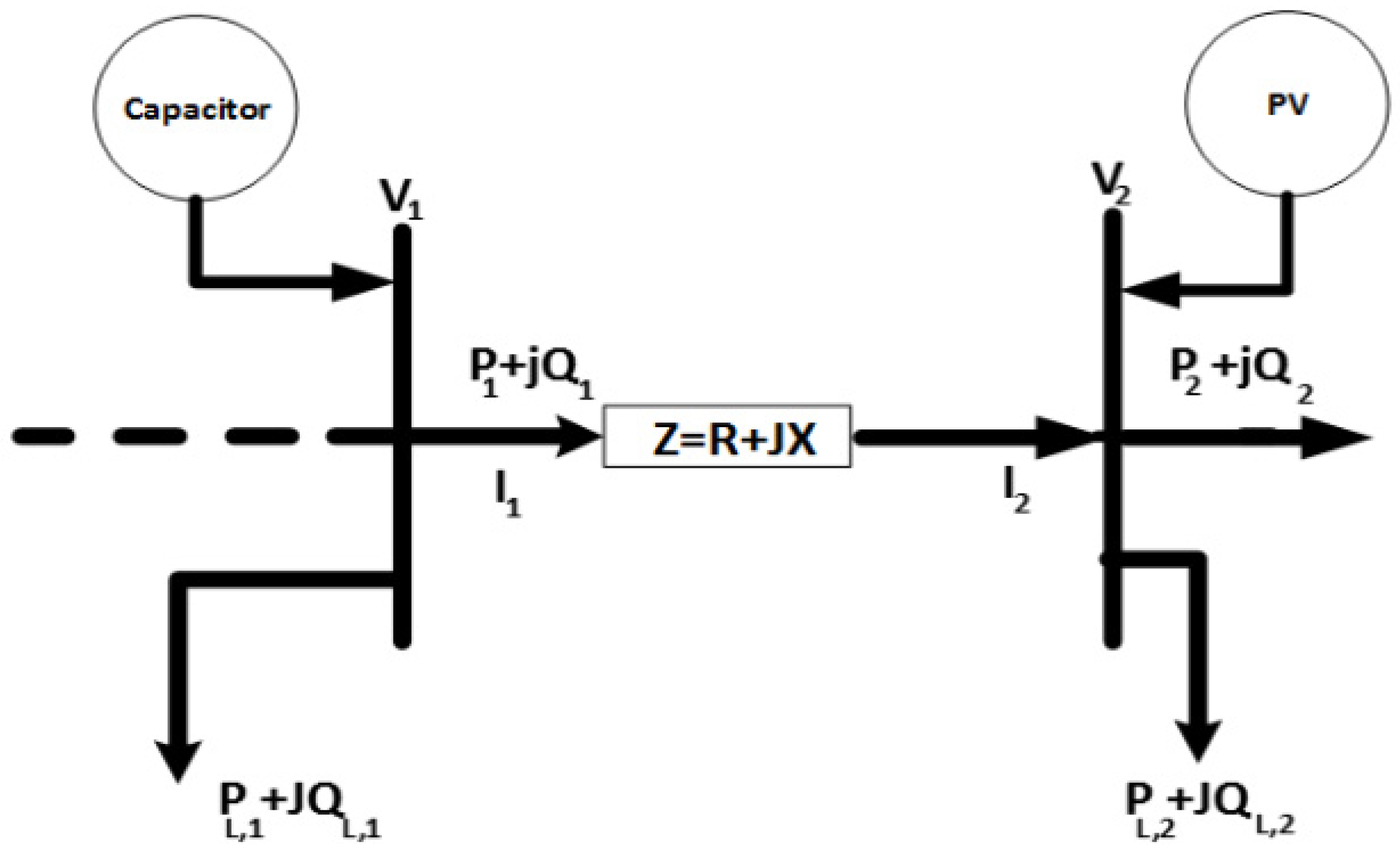
2. Problem Formulation

Figure 1 shows the representation of two buses in a distribution system.
The system power flow is evaluated in a backwards direction by Equations (1) and (2) [24]:
P 1 = P 2 + P L 2 + R ( ( P 2 + P L 2 ) 2 + ( Q 2 + Q L 2 ) 2 | V 2 | 2 )
Q 1 = Q 2 + Q L 2 + X ( ( P 2 + P L 2 ) 2 + ( Q 2 + Q L 2 ) 2 | V 2 | 2 )
Then, the voltage magnitude of bus (r) can be determined in a forward direction as follows:
V 2 2 = V 1 2 2 ( P 1 R + Q 1 X ) + ( R 2 + X 2 ) ( P 1 2 + Q 1 2 ) V 1 2
The problem formulation can be presented as a multiobjective function as follows:
f t   = k 1 f 1 + k 2 f 2 + k 3 f 3
where,
f 1 = m = 1 B ( P l o s s ( m ) )
f 2 = m = 1 S ( V D ( m ) )
f 3 = 1 m = 1 S ( | V S I ( m )   | )
| k 1 | + | k 2 | + | k 3 | = 1
where, VD(m) represents the voltage deviation at bus (m), VSI(m) represents the voltage stability index at bus (m), S is the total system buses, and B is the total system branches. K1, K2, and K3 are weighting factors that are equal to 0.5, 0.25, and 0.25, respectively.
The inequality and equality constraints are determined as shown next [19,25,26].

2.1. Equality Constraints

The power flow balance equation that can be represented by (9) and (10), and the power flow equation that can be represented by (11) and (12), are the inequality constraints as shown next.
P S + m = 1 M P P V   ( m ) = m = 1 S P L , m + m = 1 B P   l o s s ( m )
Q S + m = 1 N Q C a p a c i t o r ( m ) = m = 1 S Q L , m + m = 1 B Q   l o s s ( m )
P 1 = P 2 + P L 2 + R ( ( P 2 + P L 2 ) 2 + ( Q 2 + Q L 2 ) 2 | V 2 | 2 )
Q 1 = Q 2 + Q L 2 + X ( ( P 2 + P L 2 ) 2 + ( Q 2 + Q L 2 ) 2 | V 2 | 2 )
where, QS and PS are the output reactive and real power from the grid, respectively, but QL,m and PL,m are the reactive and real load demand at bus (m), respectively. M and N are the total number of PVs and capacitors in RDS, respectively. PPV(m) and Qcapacitor(m) are the output power of PVs and capacitors at bus (m), respectively.

2.2. Inequality Constraints

The system operation constraints are the inequality constraints, which can be represented as follows:

2.2.1. System Voltage Constraints

The bus system voltage is operating between the minimum operating voltage (VDown) and the maximum operating voltage (VUp).
V d o w n V m V u p
DER Sizing Limits:
m = 1 M P P V ( m )   ( m = 1 S P L , m + m = 1 B P   l o s s ( m ) )
P P V ,   n P P V P P V , a
The PV output is operating between the minimum (PPV,n) and maximum power (PPV,a) of PVs in RDS.
Capacitor Size Limits:
m = 1 N Q C a p a c i t o r ( m ) ( m = 1 S Q L ,   m + m = 1 B Q   l o s s ( m ) )
Q C a p a c i t o r ,   n Q C a p a c i t o r Q C a p a c i t o r , a

2.2.2. Line Capacity Limits

The branches current of the system is operating under operating constraints:
I m I a , m   m = 1 ,   2 ,   3 ,   ,   NBr
where, Ia,m represents the high operating current in the branch (m).

3. TSA-SCA Algorithm

3.1. Tunicate Swarm Algorithm (TSA)

Tunicates are cylinder-shaped, with a gelatinous tunic that is closed at one end and open at the other. Tunicates shine with bioluminescence, generating a faint green-blue light, which can be viewed from several meters away. The size of tunicates is a few millimeters. In the ocean, tunicates absorb water to generate jet propulsion from their open ends using atrial siphons. Tunicates move in water by generating jet propulsion. The updating position of tunicates can be formulated as follow:
P p ( x ) = { F S + A   ·   P D             , i f   r r a n d 0.5 F S A   ·   P D             , i f   r r a n d < 0.5
M = | P m i n + c 1 · ( P m a x P m i n ) |
A = G M
G = c 2 + c 3 F
F = 2 c 1
P D = | F S r r a n d · P p ( x ) |
Tunicates move in a swarm in nature, which can be modeled by the following equation:
P p ( x + 1 ) = P p ( x ) + P p ( x + 1 ) 2 + c 1

3.2. Sine-Cosine Algorithm (SCA)

The SCA is derived from the cosine and sine function to create an effective optimization algorithm. The effectiveness of the SCA is based on its exploitation and exploration phases. r1 is used to balance the exploitation and exploration rates for the SCA over the course of iterations to obtain the global optimum solutions. The position of the SCA is updated as follows:
X i T + 1 =   X i T   + r 1 cos   ( r 2 ) | r 3 P i T X i T | ,   r 4 0.5
X i T + 1 =   X i T   + r 1 cos   ( r 2 ) | r 3 P i T X i T | ,   r 4 < 0.5
r 1 = 2 2 T T m a x
r 2 = 2   rand   ( )
r 3 = 2   rand   ( )
r 4 =   rand   ( )
Where, Tmax and T are the maximum and current iteration, respectively, PiT is the targeted global optimal solution, and XiT represents the current iteration. r1, r2, r3, and r4 are random numbers.

3.3. Improved TSA-SCA Algorithm

The improved TSA-SCA is created by applying the updating position of the SCA to the updating position of the TSA to improve the exploration phase of the TSA. The rest of the pseudo code of the TSA remains the same, as shown in the following equations:
P D = r a n d ( ) sin ( r a n d ( ) ) | F S r r a n d · P p ( x ) | ,   rand   ( ) < 0.5
P D = r a n d ( ) cos ( r a n d ( ) ) | F S r r a n d · P p ( x ) | ,   rand   ( ) < 0.5
P p ( x ) = { F S + A   ·   P D     ,   i f   r r a n d 0.5 F S A   ·   P D     ,   i f   r r a n d < 0.5
P p ( x + 1 ) = P p ( x ) + P p ( x + 1 ) 2 + c 1
The steps of the TSA-SCA to determine the optimal sizes and locations of DG in distribution networks are explained in the following steps:
  • Read the system data, maximum iteration (I), and number of search agents (S).
  • Produce the initial population of slime mold between the lower-(w) and upper (p)-controlled variables by Equation (36).
    J ( c , q ) = r a n d ( R ( c , q ) y ( c , q ) ) + y ( c , q )
    where, r a n d represents a random value between the values of 0 and 1.   c and q are the number of tunicates and the problem dimension.
  • The produced population represents the tunicate position that can be formulated as follows:
    S = [ S 1 , 1 S 1 , 2 S 1 , q 1 S 1 , q S 2 , 1 S 2 , q 1 S 2 , q S N , 1 S N , q 1 S N , q ]
    where, S i , j is the position of the tunicate.
  • Evaluate the fitness for all locations of tunicates, and obtain the superior position of tunicates and the superior objective function.
  • Evaluate the new position of each tunicate by Equation (35).
  • Return to step 4 until the final iteration is reached.
  • Obtain the best location of tunicates (sizes and positions of DG).

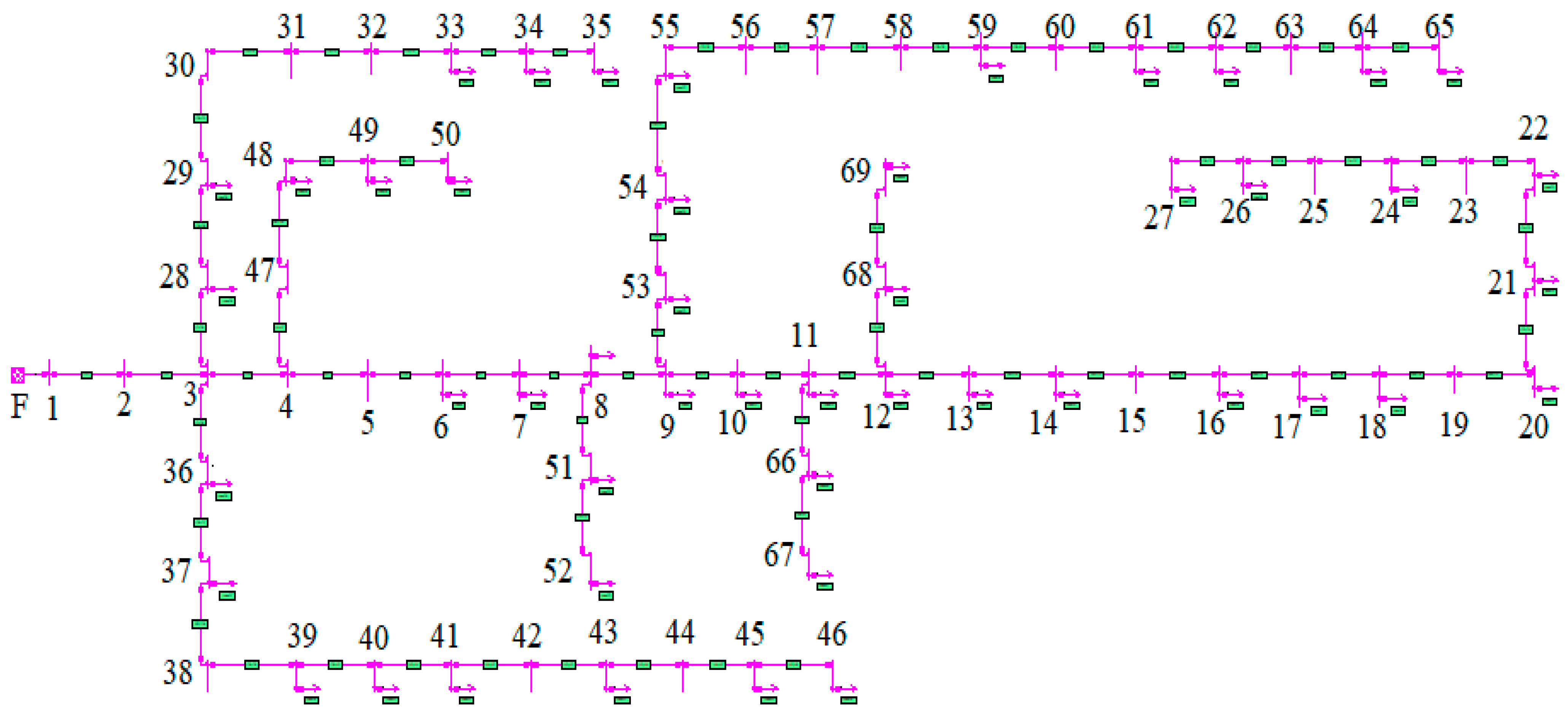
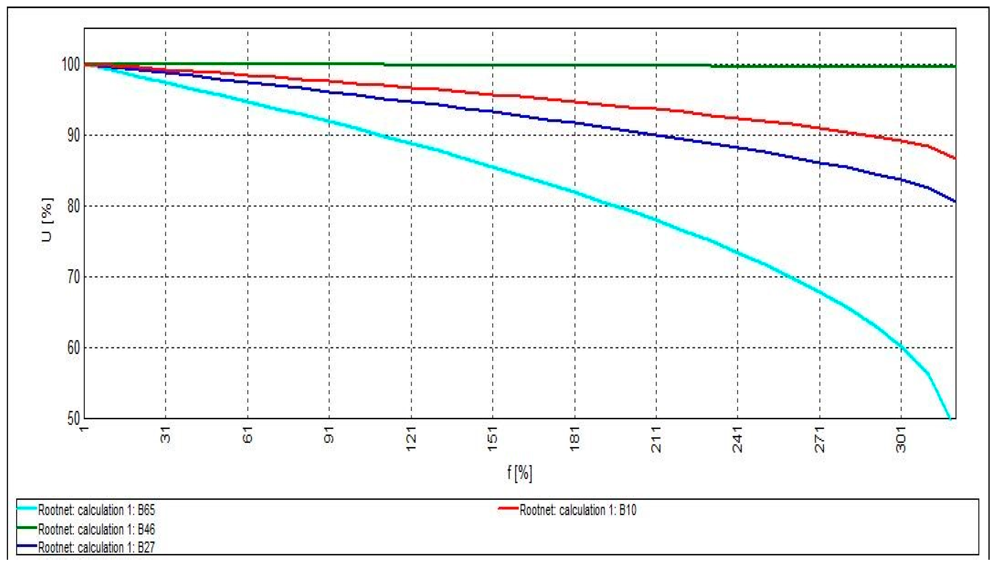
4. Testing and Evaluation

As mentioned in Section 1, the proposed optimization method is applied to the IEEE 69-node RDS to identify the optimal sizing and allocation of DG in such a system, considering the minimization of power losses. Such a system is tested by the proposed method when installing one, two, and three DGs to it. Also, the DG mode changes, i.e., DG is tested in three modes: while generating active power only (P-type mode), while generating reactive power only (Q-type mode), and while generating both active and reactive power.
The presented test system is a IEEE 69-node RDS that includes load demand of 3801.49 kW and 2694.6 kVAR [23]. This system consists of 69 buses and 68 branches with a base of 12.66 kV and 100 MVA. Figure 2 shows the system implementation by NEPLAN software.
The analysis of the IEEE 69-node RDS system in its original case shows the active power losses of the system (PLosses = 225 kW), and the least voltage is in node 65, where the voltage of that node is V65 = 0.9092 pu. Figure 3 shows the loading ability of the system by PV curves, where PV curves are applied on buses 10, 27, 46, and 65.
The PV curves show that the voltage of node 65—the weakest node in the RDS—starts to fall below 90% of nominal voltage when loads exceed 110%, and the system collapses when loads exceed 320%. Now the hybrid TSA-SCA method can start to be used to optimize the system by identifying the optimal allocation and sizing of DG installed regarding active power losses. After the optimization process, the system is analyzed to show the impact of the optimization process on the performance of the system. The optimization process is achieved using MATLAB R2019b on a personal computer with 2 GB RAM and Intel(R) Pentium(R) CPU B950, 2.1 GHZ, while the analyses are achieved using NEPLAN software.

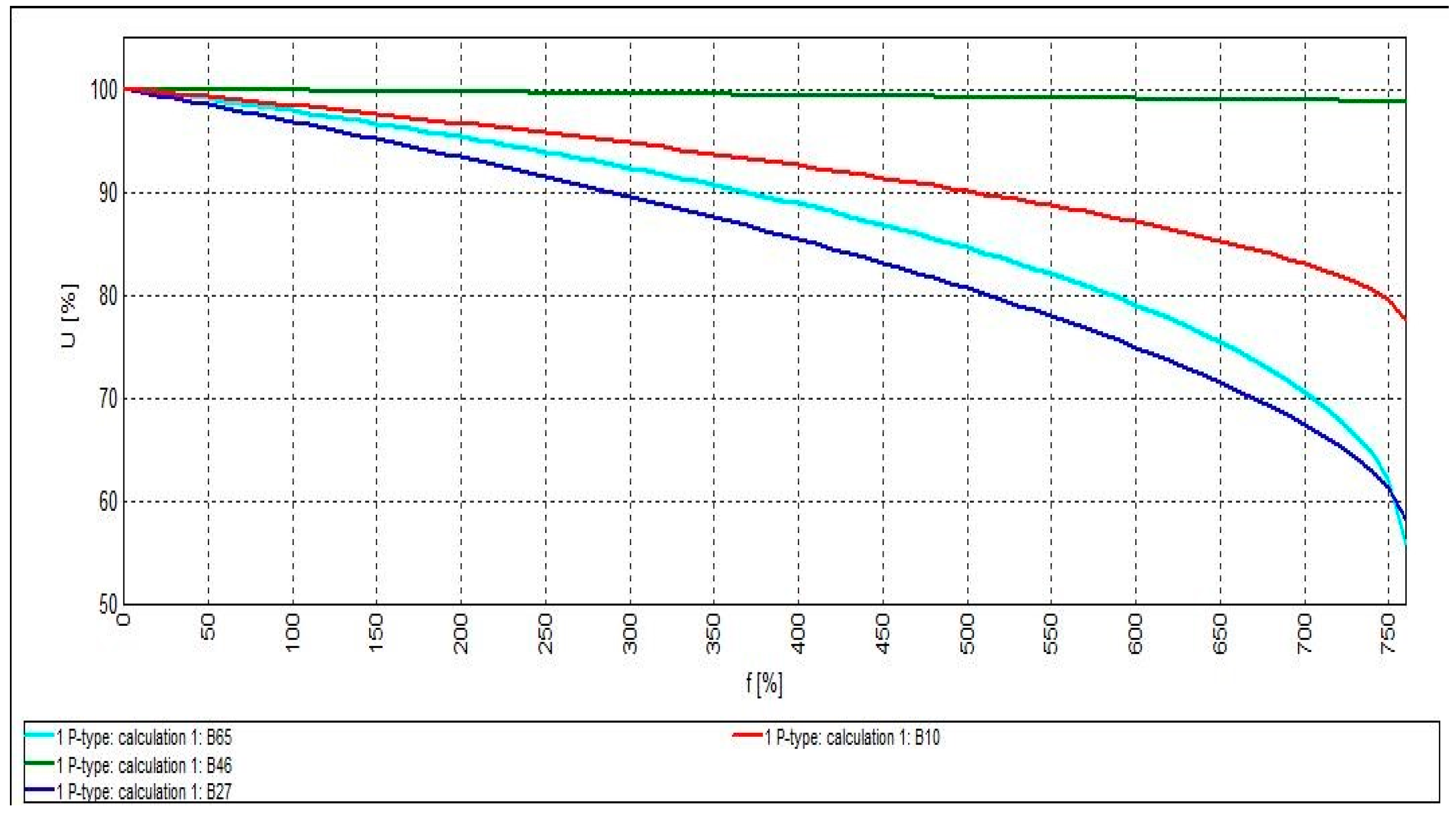
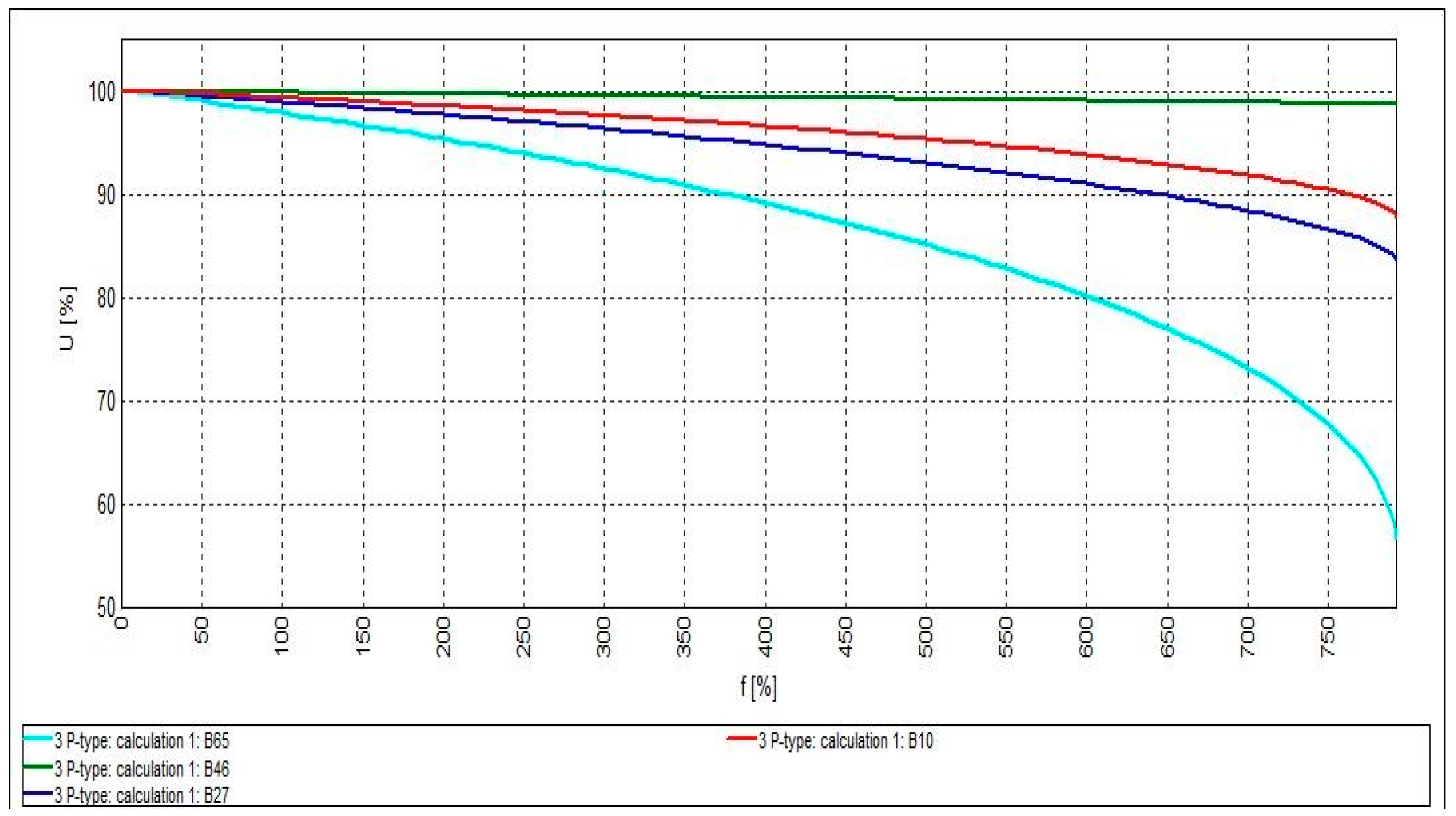
4.1. System Optimization with Active Power-Generating DG (P-Type Mode)

In this case, the DGs installed are P-type and are configured for system optimization regarding the objective function as it is shown in Table 1.
According to the settings of DGs shown in Table 1, the load flow process and PV curves were carried out. Starting with the system with one DG installation, results show power loss (Ploss = 83.2224 kW), and the total power loss reduction = 63.012%. The least voltage is found in node 27, where V27 = 0.9683 pu. Figure 4 shows the system’s PV curves with one P-type DG installation.
Due to the new DG’s location, the PV curve of node 65 improved, as shown in Figure 4. Figure 4 shows that the voltage of node 27—the system’s weakest node in that case—starts to fall below 90% of nominal voltage when loads exceed 290%, and the system collapses when loads exceed 750%.
When installing two P-type DGs to the system according to the settings in Table 1, the active power loss of the system is PLoss = 71.6745 kW, and the total active power loss reduction is 68.145%. The least voltage is found in node 65, where V65 = 0.9789 pu. Figure 5 shows the system’s PV curves with two P-type DG installations.
The presence of the two DGs in the estimated locations improves the PV curves even more. Figure 5 shows that the voltage of node 65—the weakest node in that case—starts to fall below 90% of nominal voltage when loads exceed 380%, and the system collapses when loads exceed 750%.
When installing three P-type DGs to the system according to the settings of Table 1, the active power loss of the system is PLoss = 69.4266 kW, and the total active power loss reduction is 69.144%. The least voltage is found in node 65, where V65 = 0.979 pu. Figure 6 presents the system’s PV curves with three P-type DG installations.
Figure 6 shows that there is almost no drastic effect on the system’s PV curves when installing 3 P-type DGs. The voltage of node 65—the system’s weakest node in that case—starts to fall below 90% of nominal voltage when loads exceed 380%, and the system collapses when loads exceed 750%. It is also observed that the presence of the third DG resulted in an improvement on node 10′s PV curve.

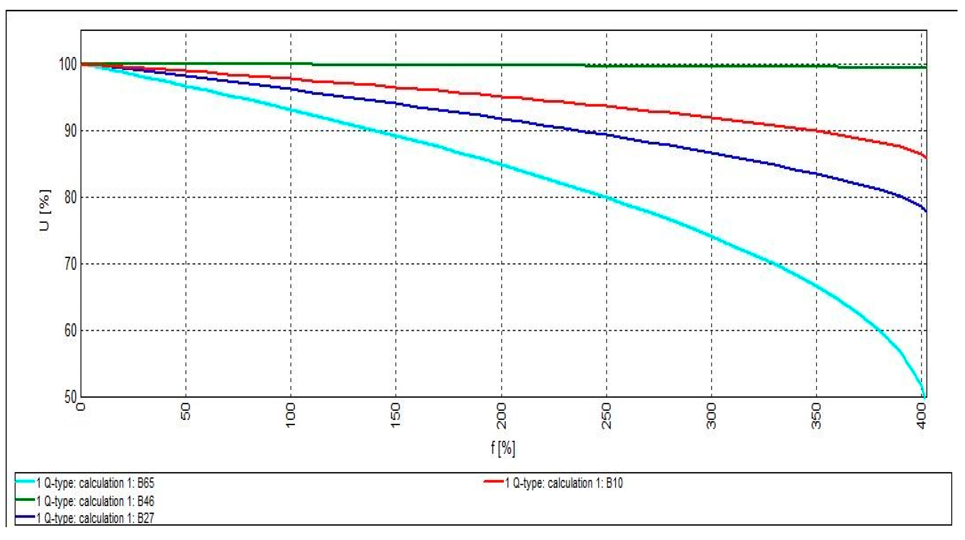
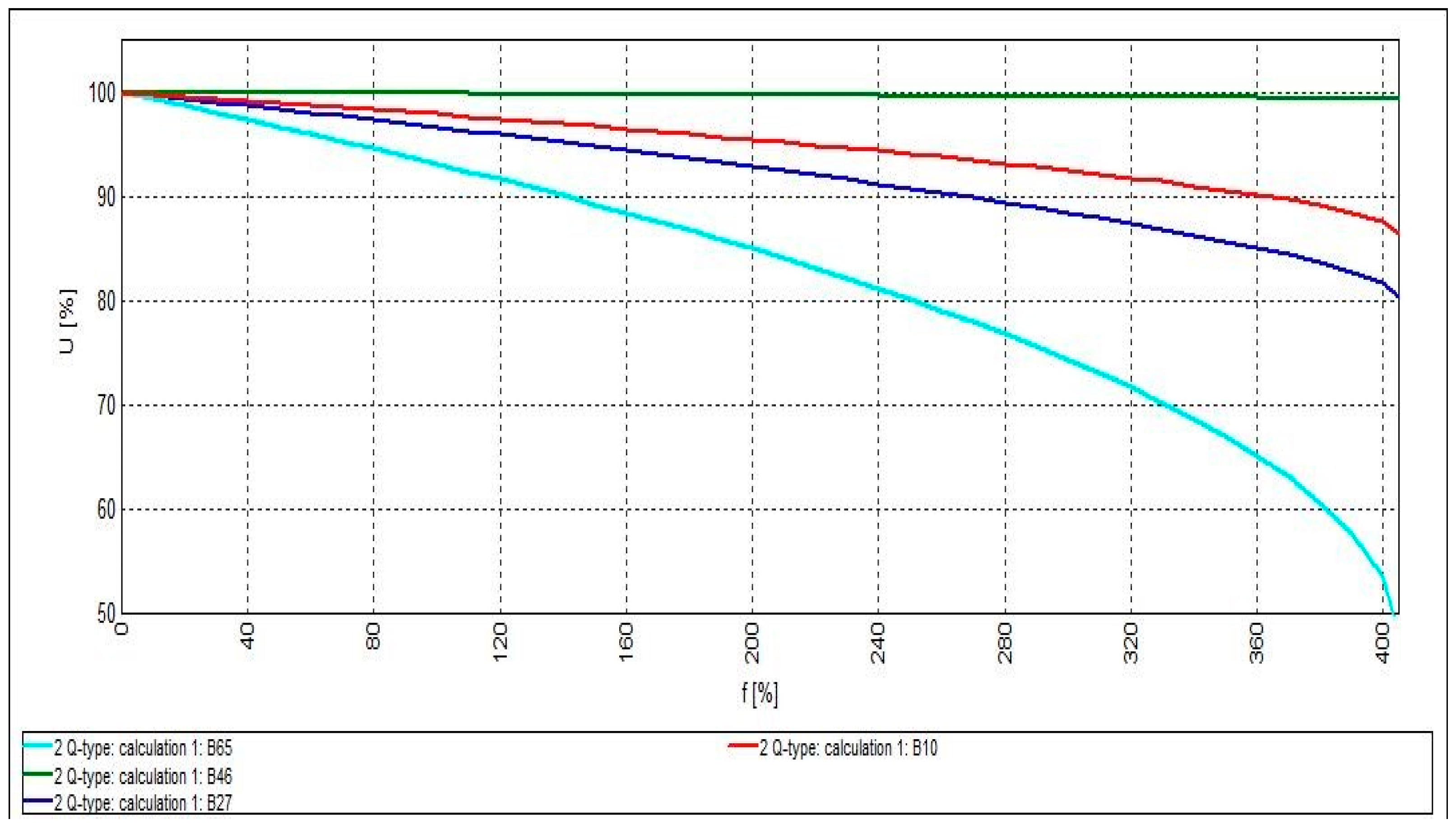
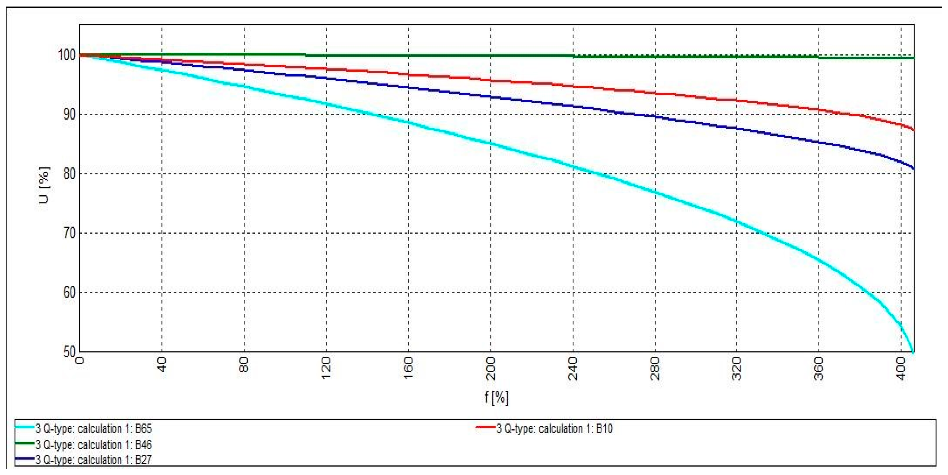
4.2. System Optimization with Reactive Power-Generating DGs (Q-Type Mode)

In this case, the DGs installed are Q-type DGs and are configured for system optimization regarding the objective function as it is shown in Table 2.
Following the settings of DGs shown in Table 2, the load flow process and PV curves were carried out. When installing one Q-type DG, the power loss of the system is PLoss = 152.041 kW, and the total power loss reduction = 32.426%. The least voltage is found in node 65, where V27 = 0.9307 pu. Figure 7 presents the system’s PV curves with one Q-type DG installation.
In the presence of one Q-type DG, the system’s PV curves improved. Figure 7 shows that the voltage of node 65—the system’s weakest node in that case—starts to fall below 90% of nominal voltage when loads exceeds 140%, and the system collapses when loads exceeds 400%.
When installing two Q-type DGs to the system according to the settings in Table 2, the active power loss of the system is PLoss = 146.441 kW, and the total active power loss reduction is 34.915%. The least voltage is found in node 65, where V65 = 0.9311 pu. Figure 8 presents the system’s PV curves with two Q-type DG installations.
Figure 8 shows that there is almost no drastic effect on the system’s PV curves when installing 2 Q-type DGs. The voltage of node 65—the system’s weakest node in that case—starts to fall below 90% of nominal voltage when loads exceed 140%, and the system collapses when loads exceed 400%.
When installing three Q-type DGs to the system according to the settings of Table 2, the active power loss of the system is PLoss = 145.129 kW, and the total active power loss reduction is 35.498%. The least voltage is found in node 65, where V65 = 0.9314 pu. Figure 9 presents the system’s PV curves with three Q-type DG installations.
Again, Figure 9 shows that there is almost no drastic effect on the system’s PV curves when installing 3 Q-type DGs. The voltage of node 65—the system’s weakest node in that case—starts to fall below 90% of nominal voltage when loads exceed 140%, and the system collapses when loads exceed 400%.

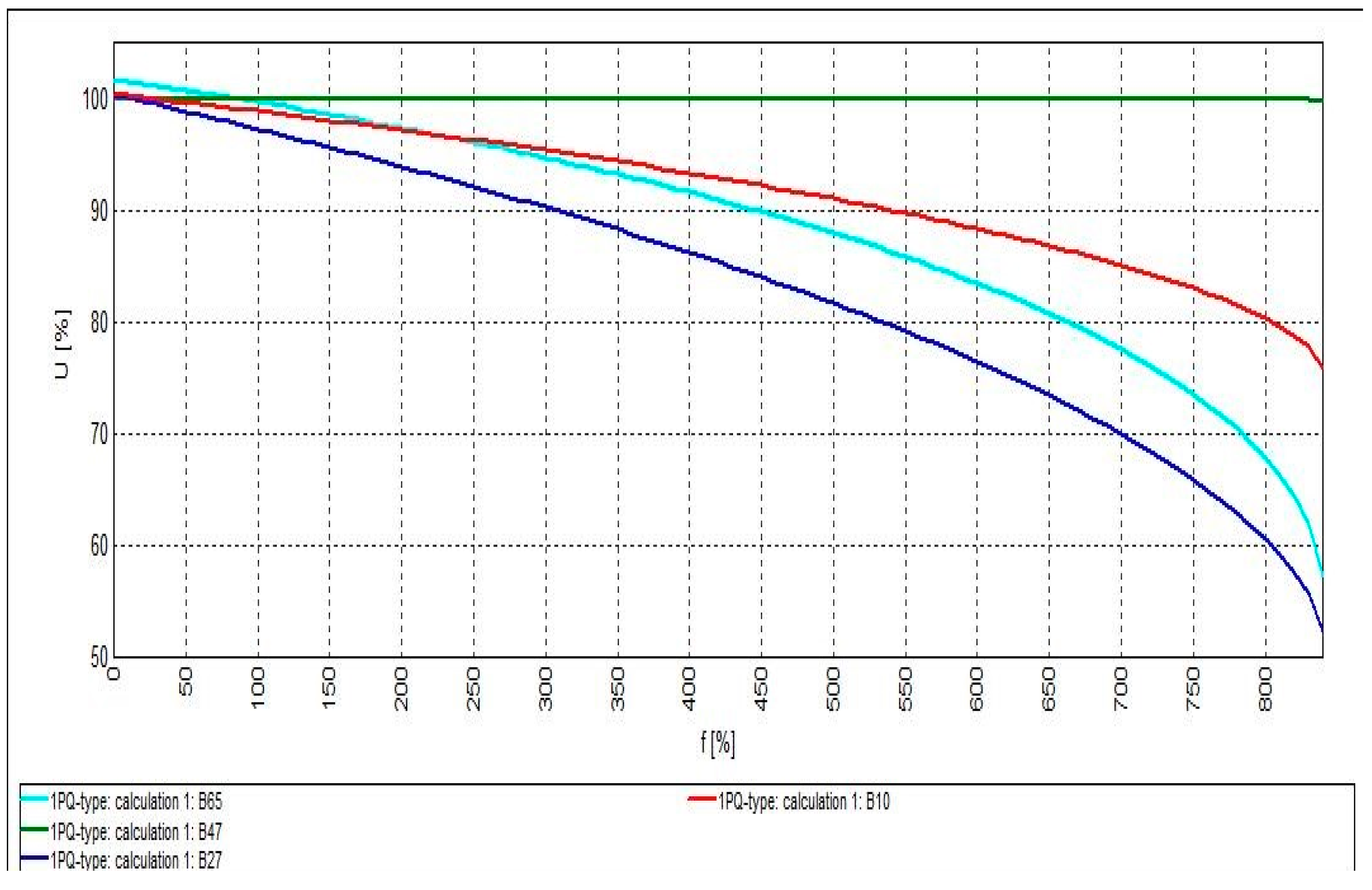
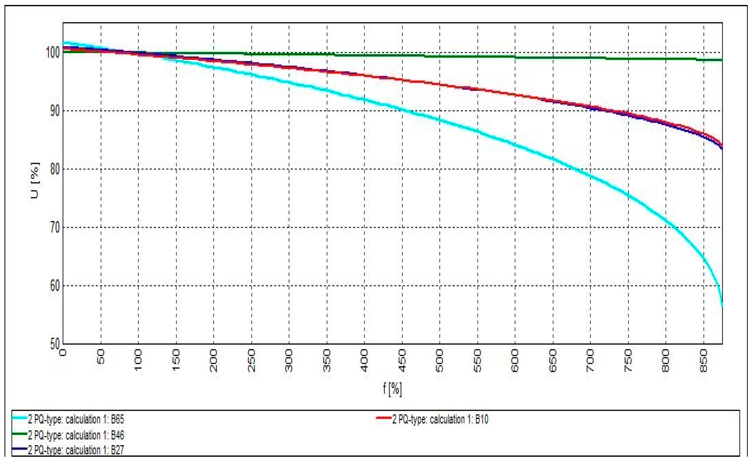
4.3. System Optimization with Active and Reactive Power-Generating DG (PQ-Type Mode)

In this case, the DGs installed are PQ-type DGs and are configured for system optimization regarding the objective function as it is shown in Table 3.
Following the settings of DGs shown in Table 3, the load flow process and PV curves were carried out. When installing one PQ-type DG, the power losses, PLoss = 23.169 kW, and the total power loss reduction = 89.702%. The least voltage is found in node 27, where V27 = 0.9725 pu. Figure 10 presents the system’s PV curves with one PQ-type DG installation.
Due to the presence of the powerful PQ-type DG, the system’s PV curves acquired superior improvement, as the DG provides both active and reactive power to the RDS. Figure 10 shows that the voltage of node 27—the system’s weakest node in that case—starts to fall below 90% of nominal voltage when loads exceed 310%, and the system collapses when loads exceed 850%.
When installing two PQ-type DGs to the system according to the settings in Table 3, the active power loss of the system is PLoss = 7.2013 kW, and the total active power loss reduction is 96.799%. The least voltage is found in node 69, where V69 = 0.9943 pu. Figure 11 presents the system’s PV curves with two PQ-type DG installations.
Due to the presence of the two PQ-type DGs, the system’s PV curves were improved even more. Figure 11 shows that the voltage of node 65—the system’s weakest node in that case—start to fall below 90% of nominal voltage when loads exceed 450%, and the system collapses when loads exceed 850%.
When installing three PQ-type DGs to the system according to the settings of Table 3, the active power loss of the system is PLoss = 4.2665 kW, and the total active power loss reduction is 98.104%. The least voltage is found in node 65, where V65 = 0.997 pu. Figure 12 presents the system’s PV curves with three PQ-type DG installations.
Figure 12 shows that a slight increase in the system’s load capacity happens when installing 3 PQ-type DGs in the system. The voltage of node 65—the system’s weakest node in that case—starts to fall below 90% of nominal voltage when loads exceed 460%, and the system collapses when loads exceed 850%. Even more, the PV curve of node 10 is slightly improved more than in the case of two PQ-mode DGs.
Table 4 shows the comprehensive results between TSA-SCA techniques and several other techniques.
From Table 4, the improved TSA-SCA has efficient characteristics to obtain the best results when compared to other efficient algorithms.

5. Conclusions

This paper introduces a new hybrid approach, a mixture between the tunicate swarm algorithm (TSA) and the sine-cosine algorithm (SCA) optimization technique. The new TSA/SCA optimization technique was tested on an IEEE 69-node RDS system, where the fitness is decreasing the active power loss through identifying the optimal sizing and allocation of DGs installed on the system. The optimization process took place in three modes: with active power DGs (P-mode DGs), reactive power DGs (Q-mode DGs), and with both active and reactive power DGs (PQ-mode DGs). The performance of the optimized system was evaluated by NEPLAN software to show the impact of the optimization process on the system. The analyses shows that the objective function was successfully achieved by the proposed technique, the active power loss was obviously minimized and the load demand of the system was greatly increased so that it can withstand more loads. The results proved that integration of multiple DGs gives better results than the integration of a single DG in a distribution network. Installing PQ-type optimization gives better results than the integration of P-type or Q-type.

Author Contributions

Conceptualization, A.A., H.A.-M. and S.K.; Data curation, A.A.I. and F.J.; Formal analysis, S.K.; Resources, A.A. and H.A.-M.; Methodology, A.A.I. and F.J.; Software, A.A., H.A.-M. and S.K.; Supervision, A.A.I. and F.J.; Validation, A.A. and S.K.; Visualization, H.A.-M., A.A.I. and F.J.; Writing—original draft, A.A., H.A.-M. and S.K.; Writing—review & edit-ing, A.A.I. and F.J. All authors together organized and refined the manuscript in the present form. All authors have approved the final version of the submitted paper. All authors have read and agreed to the published version of the manuscript.

Funding

This research was funded by NSFC (China)-ASRT (Egypt) Joint Research Fund grant number 51861145406.

Institutional Review Board Statement

Not applicable.

Informed Consent Statement

Not applicable.

Data Availability Statement

Not applicable.

Acknowledgments

The authors gratefully acknowledge the contribution of the NSFC (China)-ASRT (Egypt) Joint Research Fund, Project No. 51861145406 for providing partial research funding to the work reported in this research.

Conflicts of Interest

The authors declare no conflict of interest.

References

  1. Abdmouleh, Z.; Gastli, A.; Ben-Brahim, L.; Haouari, M.; Al-Emadi, N.A. Review of optimization techniques applied for the integration of distributed generation from renewable energy sources. Renew. Energy 2017, 113, 266–280. [Google Scholar] [CrossRef]
  2. Mekhilef, S.; Saidur, R.; Kamalisarvestani, M. Effect of dust, humidity and air velocity on efficiency of photovoltaic cells. Renew. Sustain. Energy Rev. 2012, 16, 2920–2925. [Google Scholar] [CrossRef]
  3. Rizzi, F.; van Eck, N.J.; Frey, M. The production of scientific knowledge on renewable energies: Worldwide trends, dynamics and challenges and implications for management. Renew. Energy 2014, 62, 657–671. [Google Scholar] [CrossRef]
  4. Paska, J.; Biczel, P.; Kłos, M. Hybrid power systems–An effective way of utilising primary energy sources. Renew. Energy 2009, 34, 2414–2421. [Google Scholar] [CrossRef]
  5. Raheem, A.; Abbasi, S.A.; Memon, A.; Samo, S.R.; Taufiq-Yap, Y.H.; Danquah, M.K.; Harun, R. Renewable energy deployment to combat energy crisis in Pakistan. Energy Sustain. Soc. 2016, 6, 1–13. [Google Scholar] [CrossRef] [Green Version]
  6. Ashfaq, A.; Ianakiev, A. Features of fully integrated renewable energy atlas for Pakistan; wind, solar and cooling. Renew. Sustain. Energy Rev. 2018, 97, 14–27. [Google Scholar] [CrossRef] [Green Version]
  7. Zaharim, A.; Sopian, K. Prospects of life cycle assessment of renewable energy from solar photovoltaic technologies: A review. Renew. Sustain. Energy Rev. 2018, 96, 11–28. [Google Scholar]
  8. Abdel-mawgoud, H.; Kamel, S.; Ebeed, M.; Aly, M.M. An efficient hybrid approach for optimal allocation of DG in radial distribution networks. In Proceedings of the 2018 International Conference on Innovative Trends in Computer Engineering (ITCE), Aswan, Egypt, 19–21 February 2018; pp. 311–316. [Google Scholar]
  9. Engelen, P.J.; Kool, C.; Li, Y. A barrier options approach to modeling project failure: The case of hydrogen fuel infrastructure. Resour. Energy Econ. 2016, 43, 33–56. [Google Scholar] [CrossRef] [Green Version]
  10. Ranieri, L.; Mossa, G.; Pellegrino, R.; Digiesi, S. Energy recovery from the organic fraction of municipal solid waste: A real options-based facility assessment. Sustainability 2018, 10, 368. [Google Scholar] [CrossRef] [Green Version]
  11. Di Corato, L.; Moretto, M. Investing in biogas: Timing, technological choice and the value of flexibility from input mix. Energy Econ. 2011, 33, 1186–1193. [Google Scholar] [CrossRef]
  12. Huisman, K.J.; Kort, P.M. Strategic technology adoption taking into account future technological improvements: A real options approach. Eur. J. Oper. Res. 2004, 159, 705–728. [Google Scholar] [CrossRef] [Green Version]
  13. Kaur, S.; Awasthi, L.K.; Sangal, A.L.; Dhiman, G. Tunicate swarm algorithm: A new bio-inspired based metaheuristic paradigm for global optimization. Eng. Appl. Artif. Intell. 2020, 90, 103541. [Google Scholar] [CrossRef]
  14. Mirjalili, S. SCA: A sine cosine algorithm for solving optimization problems. Knowl. Based Syst. 2016, 96, 120–133. [Google Scholar] [CrossRef]
  15. Reddy, P.D.P.; Reddy, V.V.; Manohar, T.G. Whale optimization algorithm for optimal sizing of renewable resources for loss reduction in distribution systems. Renew. Wind Water Sol. 2017, 4, 1–13. [Google Scholar] [CrossRef] [Green Version]
  16. Thangaraj, Y.; Kuppan, R. Multi-objective simultaneous placement of DG and DSTATCOM using novel lightning search algorithm. J. Appl. Res. Technol. 2017, 15, 477–491. [Google Scholar] [CrossRef]
  17. Syed, M.S.; Injeti, S.K. Simultaneous optimal placement of DGs and fixed capacitor banks in radial distribution systems using BSA optimization. Int. J. Comput. Appl. 2014, 108. [Google Scholar]
  18. Lalitha, M.P.; Babu, P.S.; Adivesh, B. Optimal distributed generation and capacitor placement for loss minimization and voltage profile improvement using Symbiotic Organisms Search Algorithm. Int. J. Electr. Eng. 2016, 9, 249–261. [Google Scholar]
  19. Barati, H.; Shahsavari, M. Simultaneous Optimal placement and sizing of distributed generation resources and shunt capacitors in radial distribution systems using Crow Search Algorithm. Int. J. Ind. Electron. Control Optim. 2018, 1, 27–40. [Google Scholar]
  20. Krueasuk, W.; Ongsakul, W. Optimal placement of distributed generation using particle swarm optimization. In Proceedings of the Australian Universities Power Engineering Conference, Melbourne, Australia, 10–13 December 2006; pp. 10–13. [Google Scholar]
  21. El-Fergany, A. Optimal allocation of multi-type distributed generators using backtracking search optimization algorithm. Int. J. Electr. Power Energy Syst. 2015, 64, 1197–1205. [Google Scholar] [CrossRef]
  22. Kumar Injeti, S.; Shareef, S.M.; Kumar, T.V. Optimal allocation of DGs and capacitor banks in radial distribution systems. Distrib. Gener. Altern. Energy J. 2018, 33, 6–34. [Google Scholar] [CrossRef]
  23. Abdelaziz, A.Y.; Ali, E.S.; Abd Elazim, S.M. Flower pollination algorithm and loss sensitivity factors for optimal sizing and placement of capacitors in radial distribution systems. Int. J. Electr. Power Energy Syst. 2016, 78, 207–214. [Google Scholar] [CrossRef]
  24. Eminoglu, U.; Hocaoglu, M.H. Distribution systems forward/backward sweep-based power flow algorithms: A review and comparison study. Electr. Power Compon. Syst. 2008, 37, 91–110. [Google Scholar] [CrossRef]
  25. Abdel-mawgoud, H.; Kamel, S.; Ebeed, M.; Youssef, A.R. Optimal allocation of renewable dg sources in distribution networks considering load growth. In Proceedings of the 2017 Nineteenth International Middle East Power Systems Conference (MEPCON), Cairo, Egypt, 19–21 December 2017; pp. 1236–1241. [Google Scholar]
  26. Ali, E.S.; Abd Elazim, S.M.; Abdelaziz, A.Y. Ant lion optimization algorithm for renewable distributed generations. Energy 2016, 116, 445–458. [Google Scholar] [CrossRef]
  27. Kansal, S.; Kumar, V.; Tyagi, B. Hybrid approach for optimal placement of multiple DGs of multiple types in distribution networks. Int. J. Electr. Power Energy Syst. 2016, 75, 226–235. [Google Scholar] [CrossRef]
  28. Reddy, V.V.C. Optimal renewable resources placement in distribution networks by combined power loss index and whale optimization algorithms. J. Electr. Syst. Inf. Technol. 2018, 5, 175–191. [Google Scholar]
  29. Biswal, S.R.; Shankar, G. Optimal Sizing and Allocation of Capacitors in Radial Distribution System using Sine Cosine Algorithm. In Proceedings of the 2018 IEEE International Conference on Power Electronics, Drives and Energy Systems (PEDES), Chennai, India, 18–21 December 2018; pp. 1–4. [Google Scholar]
  30. Aman, M.M.; Jasmon, G.B.; Solangi, K.H.; Bakar, A.H.A.; Mokhlis, H. Optimum simultaneous DG and capacitor placement on the basis of minimization of power losses. Int. J. Comput. Electr. Eng. 2013, 5, 516. [Google Scholar] [CrossRef]
  31. Nawaz, S.A.R.F.A.R.A.Z.; Bansal, A.K.; Sharma, M.P. Optimal Allocation of Multiple DGs and Capacitor Banks in Distribution Network. Eur. J. Sci. Res. 2016, 142, 153–162. [Google Scholar]
Figure 1. Representation of two buses in a distribution network.
Cleantechnol 03 00023 g001
Figure 2. IEEE 69 RDS implementation by NEPLAN.
Cleantechnol 03 00023 g002
Figure 3. PV curves of the IEEE 69-node RDS system in its original case.
Cleantechnol 03 00023 g003
Figure 4. PV curves of the IEEE 69-node RDS system with 1 P-type DG installation.
Cleantechnol 03 00023 g004
Figure 5. PV curves of the IEEE 69-node RDS system with 2 P-type DG installations.
Cleantechnol 03 00023 g005
Figure 6. PV curves of the IEEE 69-node RDS system with 3 P-type DG installations.
Cleantechnol 03 00023 g006
Figure 7. PV curves of the IEEE 69-node RDS system with 1 Q-type DG installation.
Cleantechnol 03 00023 g007
Figure 8. PV curves of the IEEE 69-node RDS system with 2 Q-type DG installations.
Cleantechnol 03 00023 g008
Figure 9. PV curves of the IEEE 69-node RDS system with 3 Q-type DG installations.
Cleantechnol 03 00023 g009
Figure 10. PV curves of the IEEE 69-node RDS system with 1 PQ-type DG installation.
Cleantechnol 03 00023 g010
Figure 11. PV curves of the IEEE 69-node RDS system with 2 PQ-type DG installations.
Cleantechnol 03 00023 g011
Figure 12. PV curves of the IEEE 69-node RDS system with 3 PQ-type DG installations.
Cleantechnol 03 00023 g012
Table 1. Configuration of P-type DGs installed on the IEEE-69 RDS.
Number of DGs123
Location/Size (kW)61/1873.3261/1781.2
17/530.5
61/1718.8
17/380.5
11/525
Power Losses (kW)83.222471.674569. 4266
Power Losses Reduction (%)63.01268.14569.144
Table 2. Configuration of Q-type DGs installed in the IEEE-69 RDS.
Number of DGs123
Location/Size (kVAr)61/133061/1276
17/361
61/1233
17/253
11/391
Power Losses (kW)152.041146.441145.129
Power Losses Reduction (%)32.42634.91535.498
Table 3. Configuration of PQ-type DG installed on the IEEE-69 RDS.
Number of DGs123
Location/Size (kVAr)/P.F61/1828.44/0.814961/1735/0.8138
17/523.24/0.829
61/1673.2/0.8136
17/377.86/0.8312
11/497.33/0.8155
Power Losses (kW)23.1697.20134.2665
Power Losses Reduction (%)89.70296.79998.104
Table 4. Comparison results of the improved TSA-SCA algorithm and other algorithms in the IEEE 69-bus RDS.
ItemTSA-SCAMFO [8]Hybrid [27]WOA [28]SCA [29]PSO [30]PVSC [31]
1P-type83.222483.22483.372----
2P-type71.674571.67971.82----
3P-type69.4266-69.52----
1Q-type152.041--152.064---
2Q-type146.441---147.762--
3Q-type145.129------
1PQ-type23.169----25.9-
2PQ-type7.201------
3PQ-type4.253-----9.63
Publisher’s Note: MDPI stays neutral with regard to jurisdictional claims in published maps and institutional affiliations.

