Accessing Insurance Flood Losses Using a Catastrophe Model and Climate Change Scenarios

Abstract

Impact Forecasting has developed a catastrophe flood model for Czechia to estimate insurance losses. The model is built on a dataset of 12,066 years of daily rainfall and temperature data for the European area, representing the current climate (LAERTES-EU). This dataset was used as input to the rainfall–runoff model, resulting in a series of daily river channel discharges. Using analyses of global and regional climate models dealing with the impacts of climate change, this dataset was adjusted for the individual RCP climate scenarios in Europe. The river channel discharges were then re-derived using the already calibrated rainfall–runoff models. Based on the changed discharges, alternative versions of the standard catastrophe flood model for the Czechia were created for the various climate scenarios. In outputs, differences in severity, intensity, and number of events might be observed, as well as the size of storms. The effect on the losses might be investigated by probable maximum losses (PML) curves and average annual loss (AAL) values. For return period 1 in 5 years for the worst-case scenario, the differences can be up to +125 percent increase in insurance losses, while for the return period 1 in 100 years it is a −40 percent decrease. There is no significant effect of adaptation measures for the return period 1 in 100 years, but there is a −20 percent decrease in the return period 1 in 5 years.

1. Introduction

Climate change is likely to be the most discussed factor in future risk due to its direct impacts on atmospheric perils and its indirect impacts on weather-driven perils, such as riverine and rainfall flooding. These trends were described by the IPCC in 2012 report [1]. Within Europe, climate change will alter the hydrologic cycle due to the expected shift in average temperatures and seasonal rainfall. This will lead to a change in flood frequencies; however, the frequency of specific flood events in different regions and year seasons might increase or decrease based on the related river segment locations and their specific climate regions in Europe. Although the main purpose of this article is to investigate changes in floods in terms of frequency and discharge, climate change should be taken to count as a whole process. As Sýs et al. [2] points out, change in the hydrological cycle is complex and will have consequences in water supply process, retention volume solutions, and in many other areas, such as integrated rescue system [3].

While predictions of the impacts of climate change on flood frequency are highly uncertain [4,5], we assume that it is possible to apply global and regional simulations to catastrophic loss models to predict the possible impacts on modelled financial insurance loss. In the insurance sector, since the long-term observation and experience is not good enough to estimate possible insurance flood losses, catastrophe models have been developed. Catastrophe modelling allows insurers and reinsurers to evaluate and manage natural catastrophe risk and create financial preparation according to every regulatory demand. The main outputs of probabilistic catastrophe models are probable maximum losses (PML) curves and average annual loss (AAL) values. A different view on losses can be provided by two types of PML curves: Aggregate Exceedance Probability (AEP) and Occurrence Exceedance Probability (OEP).

The nature of climate change in European regions is captured by Global Climate Models (GCMs). As Kay et al. mentioned in his study [4], the GCM is the main source of uncertainty in future flood frequency estimation. GCM simulation is downscaled via Regional Climate Models (RCMs) based on designed scenarios referred to as Representative Concentration Pathways (RCPs). Its trajectory is adopted by the IPCC for its fifth Assessment Report (AR5) [6]. Four pathways have been selected for climate modelling and research. They describe different climate futures depending on how much greenhouse gases are emitted in future years. The four RCPs, namely RCP 2.6, RCP 4.5, RCP 6, and RCP 8.5, are labelled after a possible range of radiative forcing values in the year 2100 (2.6, 4.5, 6.0, and 8.5 W/m², respectively). Those pathways are widely used in common studies [5,7,8,9]. The study by Rajczek et al. [9] examines the influence of future precipitation extremes. Based on their study, which investigates precipitation effected by RCP scenarios, changes in extremes do not scale proportionally to changes in mean. Basically, there is expected intensification of extrema and change in frequency of events. Single-day events intensify more than multiday precipitation. In the context of Czechia, recent changes are also examined in the research of the Czech Academy of Sciences in [10].

Floods across Europe are caused by numerous triggers. The largest and costliest floods have occurred during different seasons, in different regions, and in various regional patterns. In Czechia, flooding often occurs during the summer season, with most of the recent serious floods (e.g., 1997, 2002, and 2013) occurring during this time. Major flooding can also occur in the spring (e.g., 2006), which is induced by rain or by melting of the accumulated snowpack. There are several studies from Brázdil et al. which describe the synoptic causes of floods on the Morava River [11] and investigate past floods in Czechia [12]. The documentary evidence of past floods and their utility in flood frequency estimation is discussed in another article [13].

Considering the change in precipitation patterns during this region’s annual cycle, a change can also be anticipated in the flood regime and flood magnitudes. As changes of flood frequency curves are a long-term reflection of atmosphere conditions and soil moisture together with snow, there is strong emphasis on regional climate and runoff generation processes. Blöschl et al. [14] mentioned that there is need for a large-scale continental study. Wider studies easily demonstrate the pattern of both increase and decrease of observed discharges. Based on his results, increasing autumn and winter rainfalls resulted in increasing floods in northwest Europe. On the other hand, decreasing precipitation and increasing evaporation caused a decrease of flood events in southern Europe. Additionally, decreasing snow cover and snowmelt results in decreased flooding in Eastern Europe. The redistribution must be considered from two connected perspectives: geographically and seasonally. Such redistribution will increase the number of flood events in winter and decrease the number of events in spring, mainly due to the changes in temperature and the amount of water accumulated in the snow cover.

There are many factors which modulate the flood response, so an increase in precipitation does not necessarily mean increasing floods. Trambley et al. [15] investigates Mediterranean basins, where decreasing soil moisture caused lower floods, even though rainfall increased. Initial saturation of the soil has a strong impact, together with future changes in evaporation caused by climate change.

The reduced precipitation amount (but with increased rainfall intensities) during the original flood season might cause a slight decrease in design flows. Still, causing an increase in the average temperature might induce floods during otherwise calm winters.

Snow storage and snowmelt are factors that modulate flood response. The effects of changing snowmelt process on flood frequency curves depend on flood-generating process in the region. For Central Europe, the most relevant process is rain-on-snow [16]. The shape of flood-frequency curve is likely to flatten out at large return periods [17]. This is caused by the reduction of lying snow cover and upper energy limit for melt.

The effect of changes in a hydrological regime that yields to the altered design flows might be incorporated directly into a catastrophic flood model. To evaluate the view of risk from the climate change scenarios, a view taken from those scenarios can be deployed in the current flood model by using the same vulnerability, exposure, and flood mitigation measures. Evaluation of the direct impacts on losses from future climate effects can be made for each scenario using the current socio-economic (and other) conditions.

Rädler [18] pointed that the reinsurance view of risk is not necessarily the same as the scientific view. The main aim is on the extrema, while the mean values of distribution play only a minor role in the risk. The Impact Forecasting Flood Model for Czechia [19] with climate change scenarios is designed to evaluate financial losses caused by riverine (fluvial) and rainfall-driven (pluvial) flooding, as well as any related groundwater (off-floodplain) flooding. This model, including climate change scenarios, is found to be well suited for investigating financial losses of the possible effects of the changed hydrological regime in Europe.

2. Materials and Methods

2.1. Meteorological Inputs

2.1.1. Current Climate

The event set used for the current climate and for the development of the Impact Forecasting Flood Model for Czechia [19] is based on a long-term (12,066 years) time series of simulated daily precipitation and temperature fields over Europe. It was generated by Karlsruhe Institute of Technology [20] from the Max Planck Institute Earth System Model (MPI-ESM/ECHAMP6) global climate model (GCM) using a resolution of approximately 100 km. It was dynamically downscaled to approximately 25 km by use of a regional climate model (RCM) COnsortium for Small Scale MOdelling-Climate Limited-area Modelling Community (COSMO-CLM) CCLM5 [21].

The daily precipitation amount and daily mean temperature from two meters fields located above-ground are used as an input for the Impact Forecasting rainfall–runoff (IFRR) model (based on Hydrologiska Byråns Vattenbalansavdelning model-HBV [22]) to calculate the time series of discharges and identify flood events. Discharges from the COSMO-CLM precipitation datasets were calculated using the historical datasets (reanalysis) as the boundary condition, instead of the GCM. There are three different reanalyzes used for the boundary data: ERA-Interim [23], ERA-20C [24], and NCEP 20CR [25].

The simulated precipitation and temperature fields are corrected for bias so that they statistically match with the observed values in the period of 1950 to 2016. We performed a thorough analysis of the various bias correction methods and their effect on simulated discharges. These were then compared to the observed discharges at gauging stations.

The final stochastic meteorological dataset, the LArge Ensemble of Regional climaTE model Simulations for EUrope (LARTES-EU) dataset [21,26], serves as a consistent source of precipitation for the entirety of Europe; however, the hydrological models require a higher resolution. The precipitation and temperature fields are interpolated to a higher resolution using various statistical or machine learning algorithms. The exact methods and final resolutions vary by basin. Bilinear interpolation was used in the Danube, for example, to produce a final resolution of up to 10 km. Machine learning was used in other basins, such as the Elbe and the Oder. For the machine learning method, we used adaptable random forests, as described in He et al. [27]. Prec-DWARF (Precipitation Downscaling With Adaptable Random Forests) is a method which can outperform bilinear interpolation in precision of downscaled spatial and temporal patterns (tradeoff being significantly longer run time and the necessity to build and train the machine learning algorithm). As advised in He et al. [27], we used a double random forest approach to avoid underestimation of extreme rainfalls and also followed the advice to consider mainly adjacent cells and distance to dry cell as covariates in training the algorithm. Some other covariates (e.g., altitude, slope, temperature) were tested for significance, but did not improve the method significantly. The final algorithm trained to downscale 24.5 km grid to 6.125 km grid over the Czech basins used random forest with 10 trees to predict smaller (thus less influential) precipitation values and another independent random forest using 100 trees to predict more extreme precipitation values. The meteorological inputs with their higher resolutions provide the additional spatial variability (due to orographic effects) required for the detailed rainfall–runoff modelling.

2.1.2. Climate Scenarios

There are many climate simulations in the conditions outlined by the various time frames and scenarios [28]. To build a climate change version of the flood model, we extracted the differences between the current climate state and the temperature and precipitation in the scenarios. Those differences (on a monthly basis) were used to adjust the days in the 12,066 years of meteorological inputs for the IFRR model, which itself was used for the development of the Impact Forecasting Flood Model for Czechia [19].

The source of the key climate variables for scenarios and the reference period was chosen using [29]. The historical data covering the period of 1901 to 2020 in this dataset is based on the CRU-TS 4.05 dataset [30]. ClimateEU uses the climate data for the typical time period of 1961 to 1990 as a baseline (or reference) dataset. Preparing a complete dataset [29] included numerous sources and methods (including the PRISM methodology-Parameter-elevation Regressions on Independent Slopes Model) to cover the rain shadows and orographic precipitation in the mountainous terrain and to allow adjustments to any anomalies. The 1961 to 1990 time period represents the climate conditions at the start of the major anthropogenic changes in climate. Only a small anthropogenic warming signal, due to particulate and sulfur pollution, is seen in this period [31]. This period has been used as a reference period for long-term climate change assessments by the World Meteorological Organization.

Future climate projections consist of 15 representative GCMs (CanESM2, ACCESS1.0, IPSL-CM5A-MR, MIROC5, MPI-ESM-LR, CCSM4, HadGEM2-ES, CNRM-CM5, CSIRO Mk 3.6, GFDL-CM3, INM-CM4, MRI-CGCM3, MIROC-ESM, CESM1-CAM5, GISS-E2R) of the CMIP5 dataset corresponding to the IPCC Assessment Report 5 (IPCC 2014) [6]. Each of these models include two emissions scenarios (RCP 4.5 and RCP 8.5). Two time periods are considered: the 2050s (2041 to 2070) and the 2080s (2071 to 2100). In this study, due to combining various sources, we redefine the 2050s as (2050 to 2075) and the 2080s as (2075 to 2100). The average projected global warming increase for RCP 4.5 is +1.4 °C (±0.5) by the 2050s and +1.8 °C (±0.7) by the 2080s. For RCP 8.5, it is +2.0 °C (±0.6) by the 2050s and +3.7 °C (±0.9) by the 2080s.

The current LARTES-EU climate data in the Impact Forecasting dataset was shifted in daily steps that were in line with the scenario deltas of the temperature and precipitation variables. This was accomplished while keeping the differences between each scenario and the reference period in line with [29]. An example of an average change of seasonal precipitation over Europe for scenario RCP 8.5 in the 2080s (2075 to 2100) time period, in comparison with the reference period of 1961 to 1990, can be seen in Figure 1. Such an adjustment was made for all combinations of scenarios.

There are a varying number of seasonal wet days in the scenario simulations. The number of wet days in each month was adjusted based on the information pertaining to the number of days that achieved the threshold of precipitation, and by changing the frequency of events available in [9,10]. For the purpose of the IFRR model, evapotranspiration was also recalculated.

Strong precipitation intensifications appear (in particular for extreme rainfall events) and most are consistent in cold seasons occurring in northern Europe, according to [9]. Decreases in the total precipitation amount and frequency appear in the summer season in some areas of Europe. The largest and most significant increases in extremes are projected for the autumn and winter seasons across all regions. Median estimates of precipitation increases are often larger than +20 percent. In summer, and to some extent in the transitional seasons of spring and autumn, changes in precipitation are more complex. Reductions in the event occurrences are opposed by a concurrent intensification of those events. For the changing frequency of wet days, we used [9] and the research of the Czech Academy of Sciences in [10]. The current climate development is so far most consistent with the RCP 8.5 emissions scenario, and in some parameters, this most dramatic scenario is already being exceeded, so this scenario was used by [10] for the assessment. However, they did work with other scenarios and state that until next turn of the century, the choice of an emission scenario does not play a significant role. Apart from winter, a decrease in precipitation can be expected, especially in spring and summer, and a decrease in precipitation combined with a higher air temperature (and thus higher evaporation) will lead to longer episodes of drought. The smallest increase or even decrease in precipitation will occur in southern Moravia, Czechia. However, in terms of flood genesis, the important information is the number of days with precipitation (1, 10, 20, and 50 mm or more). These will increase as compared to the present, but the number of days with precipitation above 1 mm will not see a major change. The number of days with more than 10 and 20 mm of precipitation will continue to increase in the future, especially in winter. An increase in the number of days with greater than 50 mm of precipitation was already detected in the mid-twentieth century.

Since there are large differences between the models, we are considering the results from the medium model for the purpose of this study. The number of days with precipitation (1 mm or more) does not change much in the present or in the future, but the number of days with at least 10, 20, and 50 mm of precipitation is already changing. For the number of days with at least 10 mm in Czechia, the number increases for the near future (2021–2060) for RCP 8.5, especially in winter. Meanwhile, the number of wet days for summer months in all cases (1, 10, 20, 50 mm, and more) decreases. Overall, for the time period of 2021 to 2060, the consensus of the models is that the smallest increase in these days should occur in southern Moravia and western Bohemia, but there is a great dispersion in all model results. Alternatively, according to [10], most days with 10 mm or more of precipitation will occur in northern Moravia, the area including Prague, and southern Bohemia.

2.2. Rainfall Runoff Model

The hydrology mode in the IFRR model is a simulation used to analyze river discharge and is comprised of the following routines: a snow routine, a soil moisture routine, a response function, and a routing routine. Each of these routines needs several parameters in addition to input precipitation, temperature, and evapotranspiration. These parameters are estimated by calibration either directly, or by meta-parameters, which are the function of the various spatial datasets (soil types, altitude, and so on). Calibration of parameters is based first on the generation of 10,000 random combinations of all parameters and selection of the best option by referencing the Nash-Sutcliff coefficient. However, this approach puts too much emphasis on the daily hydrological flows, while for IF models (or any reinsurance models) only the top flood events are important, and most daily flows are discarded. To improve the usefulness for event set preparation, different weights are introduced to prefer the match in flood events over the baseline flow. This can be further improved by additional changes in parameters to provide a better fit for the seasonality of floods, duration of flood events, and volume of the flood waves. The combination of all these calibration approaches usually leads to a good resimulation of historical discharges (Figure 2), with an example of the setting of one basin in Figure 3.

The daily time series of temperatures and precipitation was used as the input of the IFRR spatially distributed rainfall–runoff model based on the HBV model [22] and calibrated for individual catchments using historical discharge data in the frame of European basins (Figure 4). The calibrated rainfall–runoff model is then forced by precipitation and temperature fields from LAERTES-EU to simulate discharges in a daily time step. The uncertainties in the simulated discharges were analyzed by testing multiple sets of rainfall–runoff model parameters.

The output of the rainfall–runoff model serves as an input to the frequency analysis for each river segment. Output discharges are used for identifying the individual events in the frame of a processed country and producing an event set at completion. Despite careful calibration of the rainfall–runoff model, we do not directly use the values of simulated discharges, but instead convert them into a frequency domain. We then define the events as the maximum return period for those river segments within a specific time period (usually about 21 days due to the insurance practice). The final footprint of each event is the composition (patching) of flood extents for individual river segments. However, the partial flood extents for the selected predefined return periods are calculated using discharges from the design flow curves, which are usually derived from long term records or provided by the local authorities, and are considered more robust than the estimates from our rainfall–runoff model.

The calibrated model parameters and the model itself were used to calculate the magnitude of flows under the changing values of precipitation, temperature, and evaporation for each climate change scenario. In this case, the model output produces discharges comparable to the current climate.

There is only one difference in using the rainfall–runoff model output for the current climate and climate scenarios. The resulting flows for the climate scenarios were labeled with the values of the return periods for individual river discharges from the frequency analysis performed on the current climate. Therefore, the return periods are produced using “current climate discharges and return periods”. This is due to the simulated flood maps being produced by deriving the design flows and 2D hydrodynamic modelling for the current climate, yet still using them for directly implementing the climate change scenarios and without the need to resimulate the flood maps.

2.3. Scenario Definition in the Loss Model

For the assessment of climate change impacts on floods in Czechia, two RCP scenarios (RCP 4.5 and RCP 8.5) and two time horizons, the 2050s (2050 to 2075) and the 2080s (2075 to 2100), were selected. These scenarios were used to evaluate the outcome when the climate conditions in the scenarios are transferred to the current world conditions. Everything is assumed to remain the same, including the level of flood protection, the type, composition and distribution of property, and loss ratio of flooded buildings, with only the events themselves behaving differently in terms of spatial extent and the intensity of the precipitation and discharges. It is important to note that this view calculates losses using the current price level and with no consideration of inflation. This pure hazard view allows for the identification of the flood types that are key in terms of the need to implement mitigation and adaptation measures. This view serves as a basis for stakeholders to initiate any necessary actions or even a chance for insurers to change their underwriting strategy.

Additionally, the four primary scenario models have been further adjusted for a basic assessment of the impact of adaptive measures. The baseline reference model within the 2D hydrodynamic simulations/flood maps already incorporates flood protection measures. However, each river segment keeps the information about the level of protection, right up to ‘no loss’ generated by the given peril. These protection levels can be adjusted to higher protection and additionally safeguard selected segments/locations. The assumptions about dike strengthening vary in the literature, for example, the EU Report Peseta V [32] works with the assumed levee strengthening for different climate scenarios by looking at a loss reduction. It indicates up to 50 percent positive impact on losses by strengthening dikes. For the climate change scenarios with adaptation for the flood model for Czechia, the following assumptions were made. Flood barrier constructions (fixed dikes, mobile barriers, polders, dams, construction of a sewerage system, and other flood protection) are a function of time and are spatially highly variable. In light of this, a simplification is necessary for the flood protection implementation in the flood model for the purpose of estimating losses in climate change scenarios.

For the 2050s (2050 to 2075) and 2080s (2075 to 2100) time periods, we assume levee strengthening (relative to the return period of flood) for riverine floods of around +25 percent and +50 percent, respectively. For pluvial floods, we assume protection strengthening of around +10 percent and +20 percent, respectively. The assumption incorporates the individual house protection by using local mobile door barriers. The assumption is applicable for estimating losses on the whole portfolio but will not be valid for a local study on individual locations.

The event set with and without an adjusted level of flood protection can be further implemented using the same procedure as the default model for the current model. It can be used in the loss calculation platform ELEMENTS, to directly estimate the risk as a baseline reference for the Impact Forecasting Flood Model for Czechia [19]. This view, with the inclusion of adaptation changes, can serve as a basis for stakeholders to determine the effectiveness of measures against the flood types that drive the losses in the climate scenarios. It can help them decide whether to initiate other measures necessary for the landscape and society.

2.4. Risk Analysis

2.4.1. Event Identification and Event Set Generation

The event set developed for the baseline reference Impact Forecasting Flood Model for Czechia is defined using 12,066 years of daily discharges, originally defined on a grid. Each river segment is controlled by the corresponding European grid cell for Czechia. The discharges come from the IFRR model that works using meteorological inputs.

Here, a flood event is defined as an overflow or inundation that comes from a river or other body of water, whether caused by rainfall, waterway operation, dam break, water runoff or other means, that causes or threatens damage. In terms of the Impact Forecasting Flood model for the Czechia, there is a need to define the additional losses caused by rainfall that complements riverine flooding.

An event, in the framework of a catastrophic flood model, is a set of individual hydrological situations reaching a specified minimum return period and arriving at a given area in a river network (fluvial flood) or catchment (pluvial flood) at the specified window of time. It is then a prescription or list of segments and catchments and a prescription for the return period of discharges of the flood or rain in that location. The event set is a list of individual events; in the case of the reference baseline flood model for Czechia within the pan-European event set, having 63,888 events within 12,066 years. An example of one event can be a situation where half of Czechia is affected by some level of flood in a given time window, with the Vltava River in Prague reaching a return period of 1 in 300 years, the Elbe River in Děčín reaching 1 in 150 years, the Ohře River in Žatec reaching a return period of 1 in 30 years, and so on. Another event may only affect a few catchments in the Jizera Mountains where only a return period of 1 in 45 years is reached.

Each river segment of the river network of Czechia is controlled by the respective grid cell from which the rainfall–runoff model is calculated. The grid is a 3D matrix containing the daily step of the discharges, where the X and Y axes define the space while the Z axis defines the time (in days and years). Events are defined in a way that is consistent with re/insurance market conditions: anything falling within a predefined window of time is declared to be the event. The market uses the “hours clause” (HC) approach, where a window of three weeks (21 days) is used to identify the event. The discharges for each cell on each day are ranked and the return period of discharge is assigned.

Identification of events in a daily time step of 12,066 years is a non-trivial optimization problem where a maximum in time and space is sought. Events are identified by an iterative approach starting from the most severe event. Each event is assumed to last 21 days. The severity of events is measured by ground-up (GU) market losses, i.e., losses prior to the application of insurance terms and conditions, and thus includes not only the hydrological situation but also the exposure distribution and vulnerability. Measuring severity using only discharges would overestimate the importance of large, unexposed mountain and foothill areas and underestimate highly exposed urban areas.

As the intensity and distribution (both spatial and temporal) of the precipitation changes, there are also changes in climate scenarios and the temporal and spatial distribution of river channel discharges. Consequently, a different number of events can be expected in each climate scenario because each event will be unique to that specific scenario. As the heavy rains driving the most substantial flood events intensify, but become shorter, the climate change scenarios will tend towards a slightly larger number of events.

The identification of events is done using the same method as that of the reference model. The only difference is that the discharges on the grid from the rainfall–runoff model are labelled by the return period, based on the frequency analysis from the original model. This solution ensures that the modified scenario-based design flows can be translated directly into the modelled hazard language of the baseline reference model. Thus, there is no need to resimulate flood extents based on the new design flows. It is important to note that in the Impact Forecasting methodology, the river discharges are simulated for river segments at specified return periods of 1 in 5, 20, 50, 100, 200, 500, 1000, and 10,000 years. For the intermediate return periods, interpolation of depths is performed during the loss calculation in the ELEMENTS.

2.4.2. Demand Surge

Demand surge is a phenomenon defined as “a sudden and usually temporary increase in the cost of materials, services, and labor due to the increased demand for them following a catastrophe” [33]. This usually occurs after exceedingly large disasters such as severe earthquakes, cyclones, or flooding. Some well-known examples of such events are the 2011 Christchurch earthquake in New Zealand, or Hurricane Katrina in the U.S.A. in 2005 [34]. A similarly strong effect was observed in the case of the 2002 floods in Czechia [35]. How and Hasson [35] noted that insurance companies incurred additional expenses to import claims adjusters because there was an insufficient number of local adjusters after each event.

There is a direct dependence of the intensity of the demand surge on the intensity of the natural disaster. Moreover, the disaster usually comes in a highly concentrated area. During reconstruction or even just removal of damaged constructions, the demand for labor and building materials, such as steel, cement, and timber, increases dramatically and quickly outstrips the supply, thereby pushing pricing increases. Oil and gas prices can also be affected. Demand surge can be quite substantial: commercial disaster modelers estimate a range of 20–50 percent, but it can be even greater [35,36].

The Impact Forecasting Flood model for Czechia incorporates the principle of demand surge. When sorting events by their size, the first event where there is some additional loss due to the demand surge starts to be applied for an event of return period 1 in 50-years loss (close to the 1997 historical event) calculated on the market portfolio. The maximum demand surge is considered +25 percent.

The application of demand surge is a simple operation. Losses per event are determined as if no material shortage has occurred. These losses are then multiplied by a coefficient derived from Czech historical claims and loss experience. At this point, the EP curve and the AAL value are calculated by standard formulas (the advantage is that it is possible to compare losses with and without the inclusion of demand surge).

For the purposes of implementing the demand surge concept in the climate scenarios, it is not possible to consider stronger demand increases in the future because such assumptions would be too uncertain. As the frequency and intensity of scenario events change in comparison to the reference model, the same values of the increase in loss need to be applied by linking the absolute losses to the market portfolio. In practice, this means that in the reference model, the range of the individual demand surge values has been determined based on the GU loss. These absolute amounts are used to map the demand surge values in the scenario models (before the demand surge is applied). For example, the loss in the EP curve from a market portfolio of between €1.3 to €1.5 billion produces a demand surge of +20 percent, and any loss for a specific one-time event from the climate scenarios in the same market portfolio will have the same demand surge value. This is regardless of whether it is determined to be at a higher or lower return period of loss. Using this approach ensures full consistency with the reference model and the ability to compare the absolute loss among models. This mapping needs to be done for each individual scenario as listed in the previous section, because the events and the losses they produce are unique among the scenarios.

2.4.3. Frequency Analysis

Due to changes of key meteorological variables in the climate scenarios that serve as the input to the rainfall–runoff model, changes can be expected in design flows in river channels and, by extension, changes in the direct flood risk in specific locations.

The major heavy rain events that generate large and severe floods are expected to become more intense, though they may occur for shorter periods of time or be more localized. This may result in moderate discharges on large rivers decreasing, but the largest discharges intensify on rivers with smaller catchment sizes.

In the reference event set, the largest floods that happen during the year usually occur (in Czechia’s case) during the summer season. However, the data show that summer rainfall decreases on average in the climate scenarios, but the number of wet days varies. Additionally, much less water is stored in snow during the winter season in the climate scenarios, so there will be less flooding from snowmelt during the early spring season. The IFRR model includes a snow routine so that, based on a precipitation and temperature dataset, it can detect precipitation state of matter and calculate the correct amount of snowpack or snowmelt for a particular day according to the specific climate change scenario.

To explain the effects resulting from the different climate scenarios, a frequency analysis was performed on the discharges of selected large and small catchments to compare the reference model to the climate scenario models. A comparison was also made of the flood seasonality and wave duration. Additionally, the total number of events identified within the event set was compared between the reference model and the climate scenario models.

3. Results

Under the most pessimistic climate scenario, meteorological changes result in an increase in the number of small or moderate floods, in terms of the magnitude of financial losses. This is caused by either a relatively low flood intensity over a large area or a high flood intensity over a smaller area. However, the area of the largest intense floods decreases, as compared to the reference scenario. This observation may result in a different view of risk: lower return periods of losses on the EP curve and a sharp increase of the AAL, while the largest loss actually decreases due to the absence of the largest area-intensive events. Combined with the decrease in direct flood risk on large rivers, strengthening dikes on these rivers will not have a substantial effect on the loss. Alternatively, strengthening dikes on smaller rivers or building flood defenses where no flood protection measures currently exist (or building defenses against pluvial flooding) might have a more substantial effect. The effect of the increasing number of smaller events during the year can be observed from the difference between the aggregate exceedance probability (AEP) curve, which is based on the sum of losses within a year, and the occurrence exceedance probability (OEP) curve, which is based on the maximum of loss within a year.

3.1. Change in Discharges

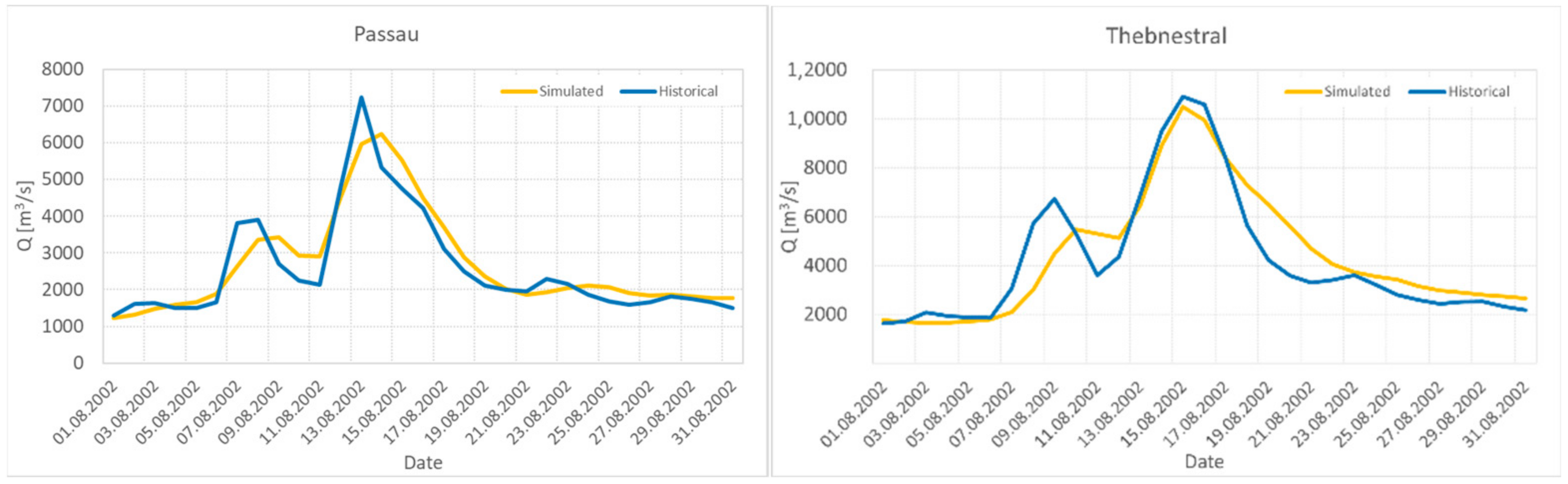
Due to the increased temperature during the cold season in the climate scenario, more of the precipitation is expected to occur as rain, rather than snow, and less water is held in the snowpack. Thus, a different runoff within the catchment can be observed. In the reference model, when the warming happens, the runoff occurs both later and suddenly, as a flood wave. In the climate scenario, the warming runoff from the basin may occur gradually and in several lower waves.

Alternately, higher flows in small catchments are observed in the climate scenario during the summer months. Although less total precipitation occurs during the summer, relatively intense but short floods occur due to the high rainfall intensity or several intense events in a row.

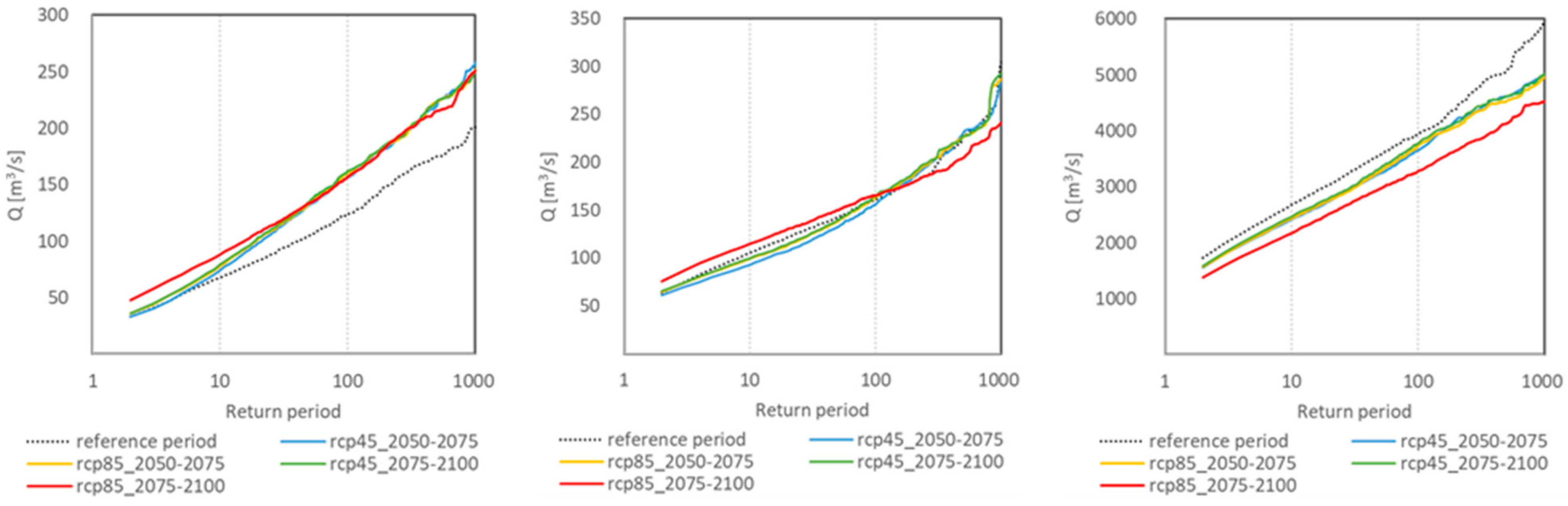
An example of the changing rainfall–runoff relationship within a watershed is shown in Figure 5. These changes are driven by the changing meteorological conditions and spatiotemporal changes in the distribution of precipitation, combined with changes in the amount of water retained in the snowpack. In large catchments, decreasing design flows can be expected under the climate scenario. For smaller catchments, the trend is the opposite and there is an increased risk of more severe flooding. It can be expected that the risk of flooding, including the risk of flooding from heavy rainfall, will be significantly increased for small catchments. For small to medium sized catchments, the magnitude of design flows increases for lower return periods but decreases for higher return periods.

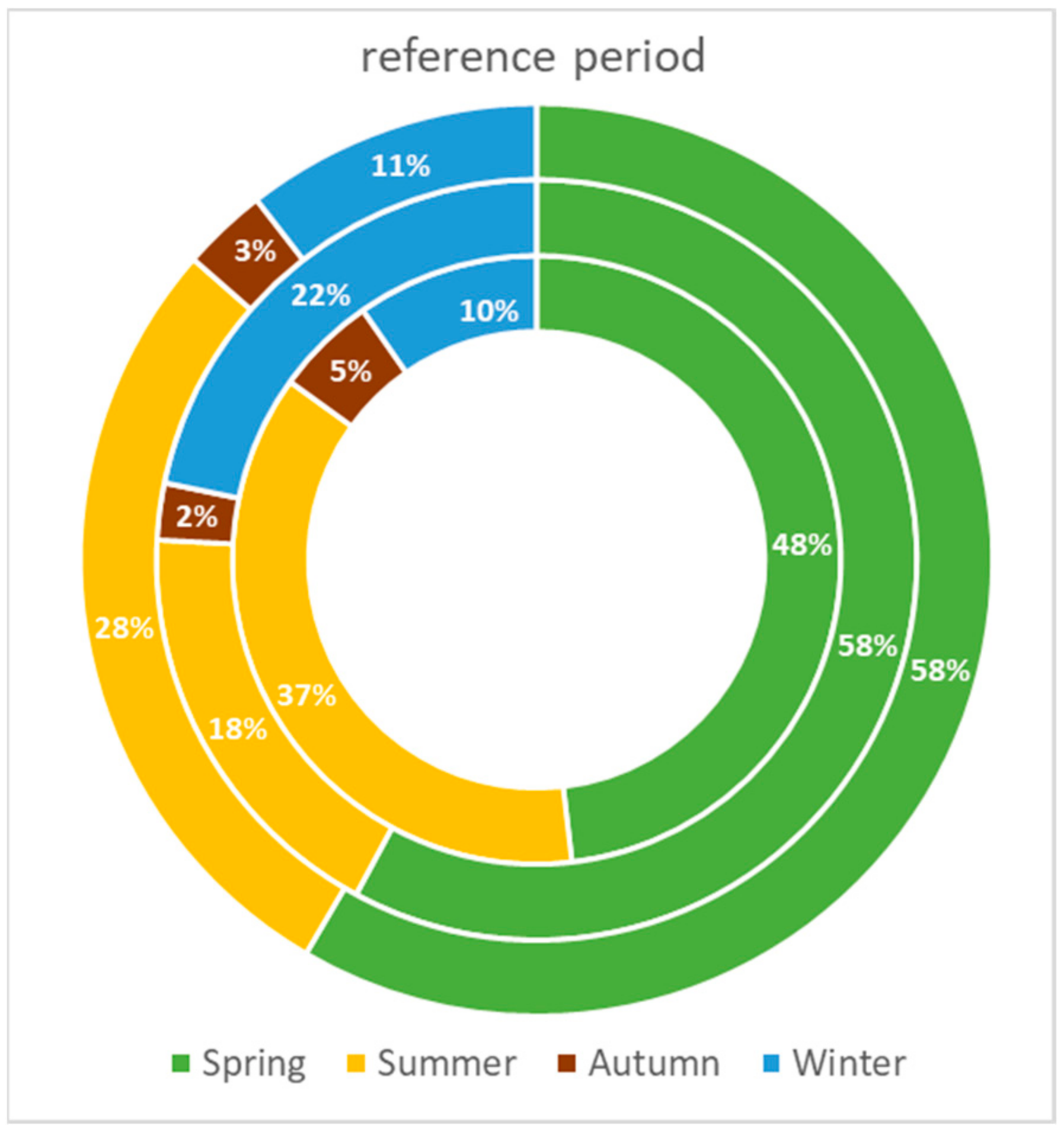
The proportion of flood events for the Czech river basins in the reference period shows that most floods greater than the return period of 1 in 20 years occur in the spring months (due to snow melting and heavy rainfall), followed by summer floods. This is illustrated by the graph in Figure 6 for the three basin sizes that were demonstrated in Figure 5. However, the largest flood peaks in the reference period occur during the summer months when the most frequent and heaviest rainfall is observed. This is also due to the given climate scenario having less rain overall in the summer months (in Czechia/Central Europe), despite the fact that there is a redistribution of wet and dry days. This redistribution then has a major effect on flood peaks in small catchments.

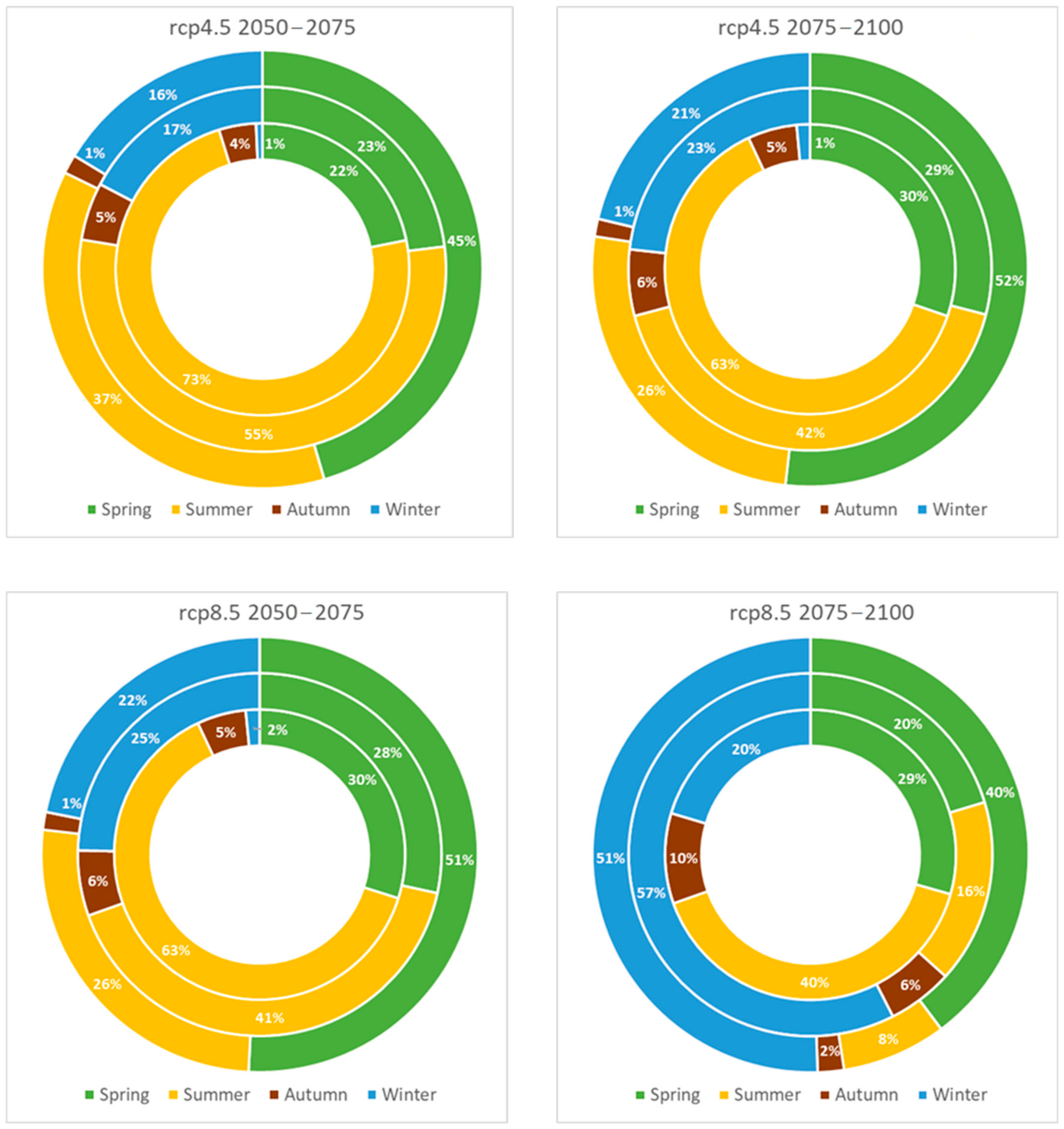
The change in the proportion of floods greater than a return period of 1 in 20 years is shown for each climate scenario (Figure 7). Due to warming over Central Europe and less water being retained in snow, there is an increase in the number of winter flood events (which are generally less damaging, but more frequent), especially in the 2080s (2075 to 2100) period and in the most pessimistic emission scenario. The number of summer floods is decreasing, but their proportion and magnitude remain significant, especially for rivers with smaller catchments.

Considering the stronger but more localized storms and rainfall events, the impact of summer floods for large catchments is limited. This is due to the need to combine several events into one using a single window. In general, floods on large catchments are generated by long lasting precipitation over a substantial area of the catchment. Consequently, the overall decrease in rainfall during the wettest period (related to the reference period) leads to an overall decrease of maximum peaks in the large catchment. Conversely, increases in rainfall in drier periods have a substantial effect on the generation of floods in the small catchments.

3.2. Number of Events

Due to the changes in the spatial and temporal distribution of precipitation and temperature (shorter periods of more intense precipitation, more water in the springtime, and so on), the response in the river network changes, as does the definition of events according to Section 2.4 (where the HC component is used). Therefore, although the number of 12,066 years of daily precipitation and temperature is constant, there is still a change in the number of events within one year. Many smaller events break down into several independent events, with the overall effect of a different ranking of events in terms of frequency. This has consequences for the calculation of the OEP and AAP loss. The number of events per scenario before flood protection applications (i.e., events defined purely in hydrological terms) is listed in

Table 1. Number of events per scenario: two time periods and two scenarios.

Scenario	Number of Events
Reference period	63,888
RCP 4.5 2050–2075	69,116
RCP 4.5 2075–2100	73,811
RCP 8.5 2050–2075	72,243
RCP 8.5 2075–2100	77,883

. The final number of events that drive the loss is smaller and depends both on the setting of local flood defenses, as well as the distribution of exposure within the portfolios.

3.3. Effect on Losses

3.3.1. Loss Change in a Multiperil Perspective

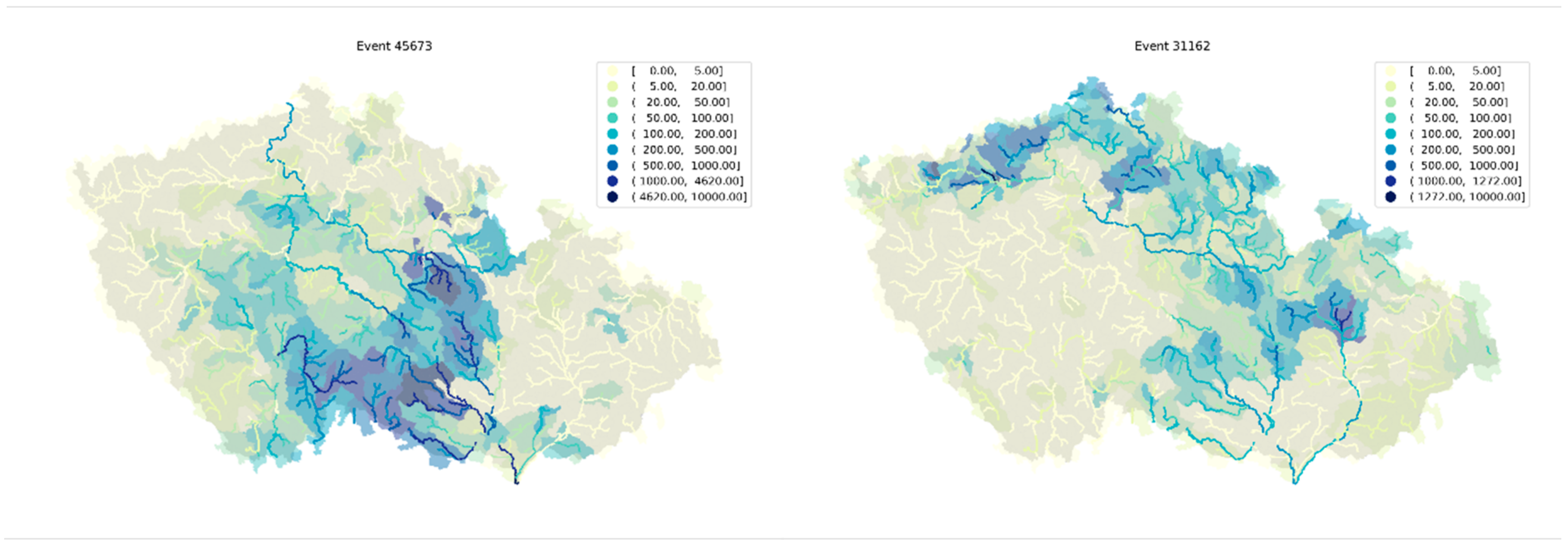
Following the definition of events in previous sections, the impact of changing climatic conditions on losses in the different climate scenarios can be demonstrated in distinct ways. The largest events for the highest emission scenarios are spatially smaller and less intense, relevant to the reference period. This is the same for the 40th–42nd largest events (which affect the return period 1 in 250-year loss), 41st shown in Figure 8. In the following sections, the relative comparison of loss magnitudes between the scenarios and the reference period can be observed. Another perspective may be to compare the first few losses. A representation of the sum of the first five to fifty losses (on the market portfolio) is shown in Figure 9. One can see that the largest (spatially) fluvial flood events are less prone to loss in the individual scenarios. This is for the reasons previously discussed. Alternatively, there are an increasing number of smaller events (locally concentrated but intense, or events less intense but (spatially) larger. A limitation of the model is that it does not necessarily capture the impact of extremely short but intense rainfall events (within the pluvial component) that may be more dominant in losses when produced from a flood model considering climate scenarios.

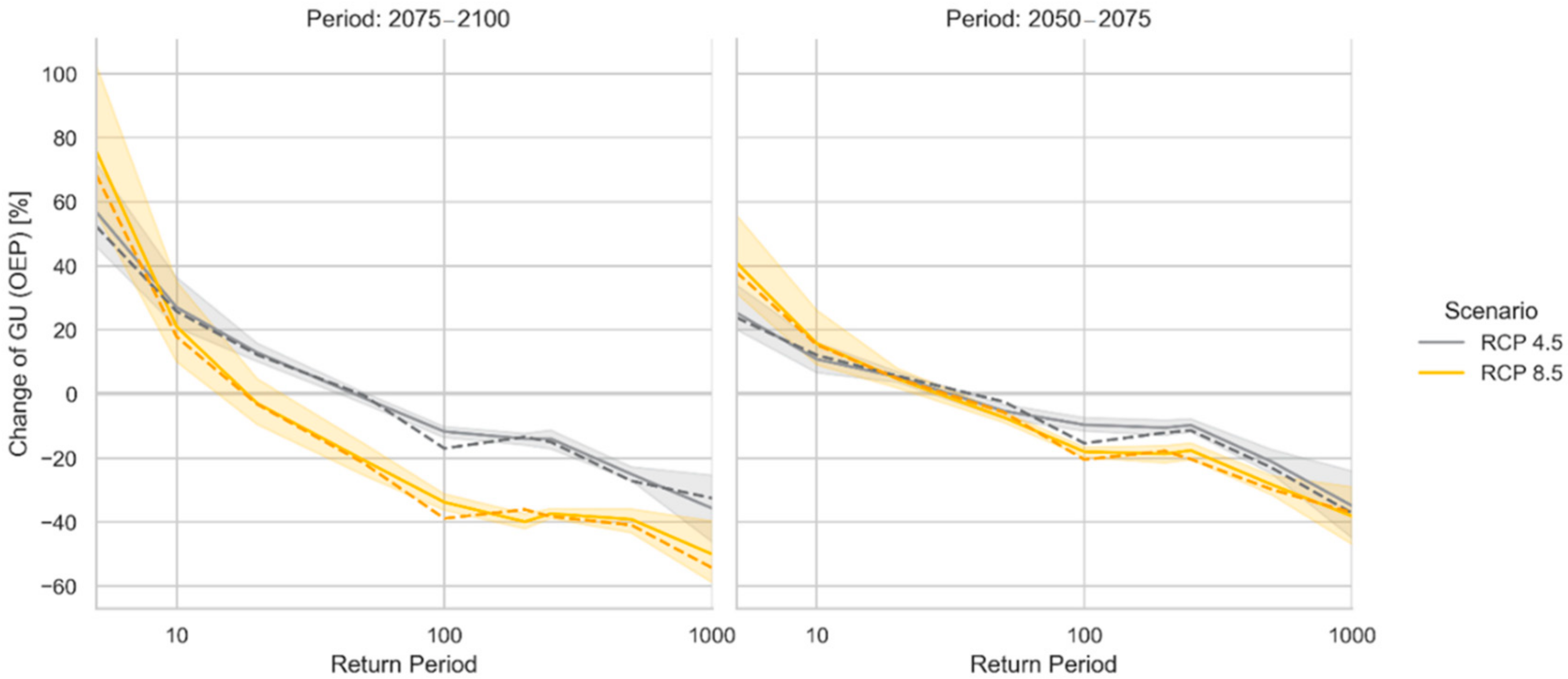
Loss analyses result not only in losses per event but also in an AAL and PML curve for each selected client portfolio. The analysis was performed using the portfolios of the seven largest Czech insurance companies and the Czech market portfolio. The PML was calculated for each scenario and period of interest for both the GU loss and the gross loss view (OEP and AEP).

By its very definition, an event set is a year-based model and the calculation of the PML is relatively straightforward. The comparison of the OEP (maximum) versus the AEP (sum of damages) is particularly interesting in terms of the frequency of the losses in the return period’s lower end of losses. The maximum return period shown on the graphs is 1 in 1000 years, but in terms of an even higher return period, the tail curve continues with an increasing trend. However, it has considerable uncertainty, and so it is not displayed.

A comparison of the PML values relative to the model results of the reference period for the variants with and without adaptation is shown in the graphs (Figure 10 and Figure 11). There is a noticeable increase in the AAL values and in the lower return periods for all scenarios and a decrease in the tail losses, with this effect being more noticeable for AEP damages than for OEP losses. At the same time, this trend is stronger for the most pessimistic emissions scenario, and the smallest changes relative to the reference period are seen in the most optimistic emissions scenario. The impact of adaptation measures (by strengthening dikes) is mainly at the tail losses. The impact on lower return periods is relatively small and caused by losses that may occur more often as a result of heavy rainfall. This is mainly owing to locations where strong protection measures cannot be expected, or small rivers with flood discharges significantly amplified will not have access to the large flood protection measures (Figure 10 and Figure 11).

3.3.2. Loss Change—Without Adaptation

This scenario assumed that key climate variables based on a specific scenario and time period are taken and transferred into the present-day climate condition. One can imagine it as if future conditions suddenly appeared in the present but everything else remained unchanged, such as the level of flood protection, spatial distribution of the exposure, loss ratio for buildings, and so on. Only the natural climate condition changed and only for the purposes of estimating the direct impact of the changes. This allows for the investigation of which hazard component and which condition will be more frequent or more important from the risk point of view. Stakeholders can then request greater details and at a more significant scale. They can also initiate real adaptation measures that are specifically targeted at the risk.

3.3.3. Loss Change—With Adaptation

As opposed to the model version, which considers climate change but from only the natural conditions, there was a developed version that includes a view of the partial adaptation measures. The original flood model for Czechia included a number of flood protections related to the river segment and the pluvial component.

Based on the table of projected strengthening of dikes in (Section 2.3), model versions with climate change scenarios and time periods have been updated with the projected levels of flood protection. The strengthening of dikes has been applied to all areas in the same ratio, so we can assume that the model can over/under-estimate the effect in more specific areas. However, other adaptation measures have not been taken into account, so we can assume that the uncertainty also covers other measures, such as the individual mobile flood barriers for doors or location-specific polders.

4. Discussion and Conclusions

This study assessed the change in risk under projected climate change scenarios, particularly in terms of their financial implications. This includes scenarios of simple climate change and scenarios with strengthened flood protection measures (to simplify, this also includes landscape measures). No additional financial implications arising from the need for levee construction or other adaptation measures are discussed in this study, nor is any loss from weather-driven perils such as windstorms, hail, or drought.

The pluvial component is considered in terms of a 24-h rainfall, for consistency with GCMs. Further research needs to be undertaken to better capture the impact of very intense but short duration torrential rainfall events on small areas and to account specifically for the impact of these storms. In terms of the rainfall–runoff model, there is a clear difference in the response of the landscape between a volume of rain that falls in six hours from a slow-moving cloud versus 24+ hours of precipitation.

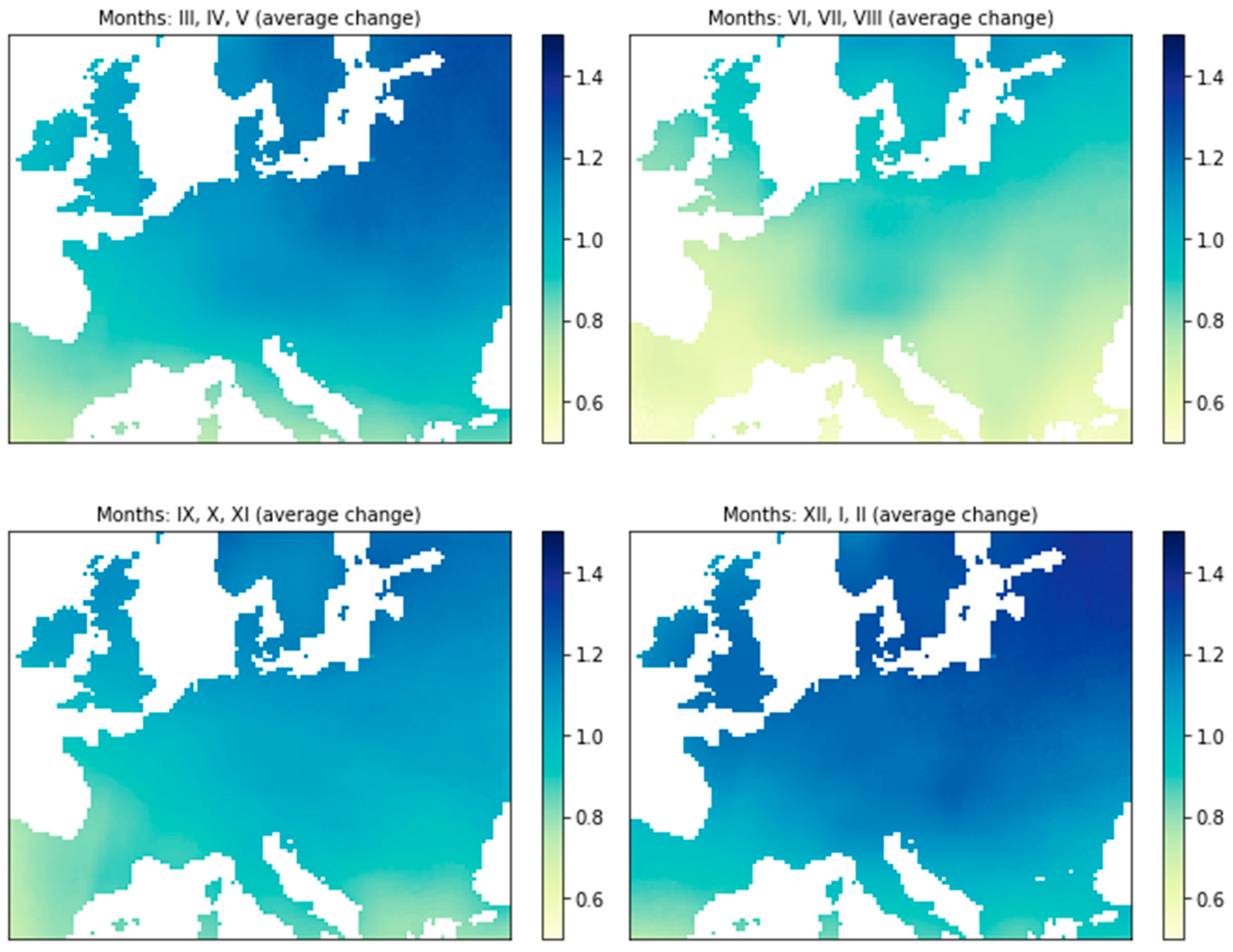
Considerable uncertainty remains in the GCM outputs about changes in precipitation totals. RCMs agree with some GCM outputs, but there are other GCMs that show no change in precipitation. According to the RCMs, precipitation will increase by an average of 10 percent by the end of the century for RCP 4.5, and even by 13 percent under RCP 8.5, as compared to the reference period (in absolute terms, this means an increase in the annual average of 90 mm for RCP 8.5 and 60 mm for RCP 4.5 by the end of this century, while the national average in the reference period is 703 mm).

Decreasing precipitation amounts are expected in the northern regions and increasing amounts in the southern regions, with the transition located across Central Europe in the summer and the southern Mediterranean in the winter. A prominent intensification of precipitation extremes is present in all seasons and nearly all regions of Europe. In the continental and northern regions, the entire set of simulations shows an increase in total precipitation around +20 percent with the largest values in winter and autumn. In southern regions, changes are more complex and particularly uncertain in warmer seasons. In those regions, the significant reduction in the number of wet days might influence the occurrence of heavy flood events in summer. Knutti, Masson, and Gettelman 2013 [37] suggest this is in line with recent observations of the European precipitation regime, such as the intensification of heavy events that particularly appears in the winter season [38,39], which is projected to amplify in a future climate. It has been reported [40] that annual average precipitation will increase in northern and North-Central Europe, while it will decrease in Southern Europe.

In Central Europe, a smaller change in precipitation is expected. However, annual precipitation patterns will change. Southern Europe will experience lower rainfall year-round. There will be less precipitation during the summer season in Atlantic and continental Europe, but more winter precipitation. It has been reported [40] that decreases in annual average precipitation in Southern and Central Europe can be as high as 30–45 percent, and up to 70 percent in the summer in some regions. Due to this and warmer summer temperatures, the risk of summer drought is likely to increase in Central Europe and in the Mediterranean area.

On the other hand, Kundzewicz et al. 2005 [41] suggested that the potential for intense precipitation is likely to increase in a warmer climate. According to the Clausius–Clapeyron Law, the atmosphere’s capacity to absorb moisture should increase with temperature. With a higher amount of precipitable water, the potential for intensive precipitation should increase. It seems likely that for broad parts of the investigation area the mean summer precipitation will decrease, corroborating the general projection of enhanced summer drying over continental interiors, while the amount of precipitation related to extreme events will increase [41]. However, the spatial size of extreme precipitation events will probably be reduced. We have observed intensification of extreme rainfall in our results, but with a reduced spatial size of storms.

Our study shows that there is very little change in total precipitation for Czechia, but the distribution of precipitation changes during the year and the number of wet and dry days also changes. This has a clear effect on runoff and flood genesis. Fewer floods are seen during spring seasons, due to the reduction of snowpack, which is consistent with predictions [9,10]. This led to a clear effect in our calibrated rainfall–runoff model for flood magnitude as well as on the superposition of flood waves. The amplification of less intense precipitation led to an amplification of flood waves on small and medium-sized catchments, while large catchments were affected by a decrease in design flows due to the stacking of flood waves. The distribution of events within the year is also changing, with an increasing number of winter floods.

Within the loss calculation where there is an increase in the loss of the lower part of the PML curve (more frequent small floods, or the splitting of a large event into several smaller ones) and a decrease in tail losses due to the reduction in the number of the largest flood events. In all climate scenarios considered, losses on the lower return periods increase and losses on the higher return periods decrease compared to the reference model. Only the magnitude of these changes differs.

The study contains several uncertainties: uncertainties in climate models, uncertainties in changing precipitation-runoff relationships in the landscape, and uncertainties in adaptation measures and in population development. To provide the most straightforward view of the estimation of the risk, the model is accordingly separated into two parts, with a portion using only the change in climate conditions for the current world and a portion using the assumption of adaptation.

This study is intended to highlight the possible trend in flood losses (without considering the price trends) and to provide a basis for further development and decision-making by the relevant institutions, the state or insurance companies. Floods over Europe are caused by various triggers. The largest and costliest floods happen in different seasons, in different regions and in different regional patterns. In Czechia, the majority of serious floods (e.g., 1997, 2002, 2013) currently happen during the summer season, but different types of flooding might dominate in the climate scenarios. Further work may target specific types of storms that do not occur in the current climate, which may play a significant role in climate scenarios. While the results of this study suggest this may be the case, the current model cannot capture this completely and without uncertainties. To evaluate the view of risk from climate change scenarios, it is possible to take a view of climate change scenarios and convey it to the current model. Using the same vulnerability, exposure, and flood mitigation measures, the evaluation of the direct impact on the losses can be achieved for each scenario of the future climate happening under current socio-economic and other conditions.

Subsequently, the effect of mankind’s efforts protecting themselves, reflected in flood mitigation, should be added to evaluate such effect. The third step in our future work is to evaluate the change in exposure (development of new residential, commercial, and industrial areas with different spatial distribution and sensitivity against flood losses) under current conditions of current costs associated with flooding.

One limitation of this study might be underestimation of the future frequency and magnitude of flash floods on small catchments due to the daily precipitation used for deriving event set and 24-h simulation of pluvial events. That might even intensify losses of lower return periods and AAL. However, hydrodynamic simulation based on derived design flows is based on a frequency analysis of extracted peaks directly from gauging stations. The output of the rainfall–runoff simulation is used only to evaluate the relative magnitude of discharge event and real flood hazard is modelled through 2-dimensional hydrodynamic simulation whose input parameters (hydrological data) are taken from intensity-duration-frequency (IDF) functions (for pluvial hazard simulations) and design flows, derived from daily maximum data. Therefore, the rainfall–runoff outputs are used only to describe the spatial patterns and relative severity magnitude of model’s stochastic events. That is why the described number of events in climate change scenarios might be considered to be comparable to the reference period.

In the studied climate scenario flood model for Czechia, for a return period 1 in 5 years for the worst-case scenario, the differences between scenario results and reference model can be up to +125 percent increase, while for the return period 1 in 100 years it is a −40 percent decrease. There is no significant effect of adaptation measures for the return period 1 in 100 years, but there is a −20 percent decrease in the return period 1 in 5 years. The study also considers exposure redistribution in addition to adaptation measures and brings attention to the significant risk of increasing tail loss in the PML curve when compared to the reference model (up to +30 percent). It also investigated pluvial flooding increases by about 10–20 percent (OEP) and 20–40 percent (AEP), respectively, in the model.

Another aim of this study was to provide a basis for the decision-making processes, which may lead to better targeting of adaptation measures in the landscape or construction of flood control measures, which may result in a significant reduction in losses from large floods of the “classic” type, as well as flood control measures in small catchments from heavy rainfall events. This may result in very different flood losses than the model projects. Stakeholders will likely wish to investigate this further, using this data to initiate processes of adaptation precisely targeted to their risk. While Impact Forecasting will continue to refine climate change scenarios in flood models to reflect new knowledge, the climate change scenarios for the Impact Forecasting Flood model for Czechia [19] considered here have been implemented into ELEMENTS so users can perform their own analyses using their portfolio data, and can make their own assumptions about exposure redistribution or price.

References

1. IPCC. Managing the Risks of Extreme Events and Disasters to Advance Climate Change Adaptation; Cambridge University Press: Cambridge, UK, 2012. [Google Scholar]
2. Sýs, V.; Fošumpaur, P.; Kašpar, T. The Impact of Climate Change on the Reliability of Water Resources. Climate 2021, 9, 153. [Google Scholar] [CrossRef]
3. Yazdani, M.; Mojtahedi, M.; Loosemore, M.; Sanderson, D. A modelling framework to design an evacuation support system for healthcare infrastructures in response to major flood events. Prog. Disaster Sci. 2022, 13, 100218. [Google Scholar] [CrossRef]
4. Kay, A.L.; Davies, H.N.; Bell, V.A.; Jones, R.G. Comparison of uncertainty sources for climate change impacts: Flood frequency in England. Clim. Chang. 2009, 92, 41–63. [Google Scholar] [CrossRef]
5. Anaraki, M.V.; Farzin, S.; Mousavi, S.F.; Karami, H. Uncertainty Analysis of Climate Change Impactson Flood Frequency by Using Hybrid Machine Learning Methods. Water Resour. Manag. 2021, 35, 199–223. [Google Scholar] [CrossRef]
6. IPCC. Climate Change 2014: Synthesis Report. In Contribution of Working Groups I, II and III to the Fifh Assessment Report of the Intergovernmental Panel on Climate Change; Cambridge University Press: Cambridge, UK, 2014. [Google Scholar]
7. Donmez, C.; Berberoglu, S.; Cilek, A.; Krause, P. Basin-wide hydrological system assessment under climate change scenarios through conceptual modelling. Int. J. Digit. Earth 2020, 13, 915–938. [Google Scholar] [CrossRef]
8. Hengade, N.; Eldho, T.I.; Ghosh, S. Climate change impact assessment of a river basin using CMIP5 climate models and the VIC hydrological model. Hydrol. Sci. J. 2018, 63, 596–614. [Google Scholar] [CrossRef]
9. Rajczak, J.; Schär, C. Projections of Future Precipitation Extremes Over Europe: A Multimodel Assessment of Climate Simulations. J. Geophys. Res. Atmos. 2017, 122, 773–800. [Google Scholar] [CrossRef]
10. Štěpánek, P.; Trnka, M.; Jan, M.; Martin, D.; Pavel, Z.; Ondřej, L.; Petr, S.; Jan, K.; Aleš, F.; Daniela, S. Expected Climatic Conditions in the Czech Republic: Part I. Change of Basic Parameters, 1st ed.; Ústav Výzkumu Globální Změny Akademie věd České Republiky: Brno, Czech Republic, 2019; ISBN 978-8-879-2-28-8. [Google Scholar]
11. Brázdil, R.; Řezníčková, L.; Valášek, H.; Havlíček, M.; Dobrovolný, P.; Soukalová, E.; Rehánek, T.; Skokanová, H. Fluctuations of floods of the River Morava (Czech Republic) in the 1691–2009 period: Interactions of natural and anthropogenic factors. Hydrol. Sci. J. 2011, 56, 468–485. [Google Scholar] [CrossRef]
12. Brázdil, R.; Dobrovolný, P.; Elleder, L.; Kakos, V.; Kotyza, O.; Květoň, V.; Macková, J.; Müller, M.; Štekl, J.; Tolasz, R.; et al. Historical and Recent Floods in the Czech Republic; Masaryk University, Czech Hydrometeorological Institute: Prague, Czech Republic, 2005; p. 370. [Google Scholar]
13. Kjeldsena, T.T.; Macdonald, N.; Lang, M.; Mediero, L.; Albuquerque, T.; Bogdanowicz, E.; Brázdil, R.; Castellarin, A.; David, V.; Fleig, A.; et al. Documentary evidence of past floods in Europe and their utility in flood frequency estimation. J. Hydrol. 2014, 517, 963–973. [Google Scholar] [CrossRef] [Green Version]
14. Blöschl, G.; Hall, J.; Viglione, A.; Perdigão, R.A.P.; Parajka, J.; Merz, B.; Lun, D.; Arheimer, B.; Aronica, G.T.; Bilibashi, A.; et al. Changing climate both increases and decreases European river flood. Nature 2019, 573, 108–111. [Google Scholar] [CrossRef]
15. Tramblay, Y.; Mimeau, L.; Neppel, L.; Vinet, F.; Sauquet, E. Detection and attribution of flood trends in Mediterranean basins. Hydrol. Earth Syst. Sci. 2019, 23, 4419–4431. [Google Scholar] [CrossRef] [Green Version]
16. Kemter, M.; Merz, B.; Marwan, N.; Vorogushyn, S.; Blöschl, G. Joint Trends in Flood Magnitudes and Spatial Extents Across Europe. Geophys. Res. Lett. 2020, 47, 7. [Google Scholar] [CrossRef] [Green Version]
17. Bertola, M.; Viglione, A.; Vorogushyn, S.; Lun, D.; Merz, B.; Blöschl, G. Do small and large floods have the same drivers of change? A regional attribution analysis in Europe. Hydrol. Earth Syst. Sci. 2021, 25, 1347–1364. [Google Scholar] [CrossRef]
18. Rädler, A.T. Invited perspectives: How does climate change affect the risk of natural hazards? Challenges and step changesfrom the reinsurance perspective. Nat. Hazards Earth Syst. Sci. 2022, 22, 659–664. [Google Scholar] [CrossRef]
19. Aon—Impact Forecasting. Impact Forecasting Flood Model for Czech Republic; Aon UK. Limited Trading as Aon: Prague, Czech Republic, 2021; 197p. [Google Scholar]
20. Ehmele, F.; Kautz, L.-A.; Feldmann, H.; He, Y.; Kadlec, M.; Kelemen, F.D.; Lentink, Y.; Manful, D.; Ludwig, P.; Pinto, J.G. Adaptation and application of the large LAERTES-EU regional climate model ensemble for modeling hydrological extremes: A pilot study for the Rhine basin. Nat. Hazards Earth Syst. Sci. 2022, 22, 677–692. [Google Scholar] [CrossRef]
21. Rockel, B.; Will, A.; Hense, A. The Regional Climate Model COSMO-CLM (CCLM). Meteorol. Z. 2008, 17, 347–348. [Google Scholar] [CrossRef]
22. Bergström, S. The HBV model. In Computer Models of Watershed Hydrology; Singh, V.P., Ed.; Water Resources Publications: Highlands Ranch, CO, USA, 1995; pp. 443–476. [Google Scholar]
23. Berrisford, P.; Dee, D.P.; Poli, P.; Brugge, R.; Fielding, M.; Fuentes, M.; Kållberg, P.W.; Kobayashi, S.; Uppala, S.; Simmons, A. The ERA-Interim Archive Version 2.0; Shinfield Park. Reading 1. 2011, p. 23. Available online: https://www.ecmwf.int/en/elibrary/8174-era-interim-archive-version-20 (accessed on 20 July 2021).
24. Poli, P.; Hersbach, H.; Dee, D.P.; Berrisford, P.; Simmons, A.J.; Vitart, F.; Laloyaux, P.; Tan, D.G.H.; Peubey, C.; Thépaut, J.-N.; et al. ERA-20C: An Atmospheric Reanalysis of the Twentieth Century. J. Clim. 2016, 29, 4083–4097. [Google Scholar] [CrossRef]
25. NOAA: The Twentieth Century Reanalysis Project. 2022. Available online: https://psl.noaa.gov/data/20thC_Rean/ (accessed on 7 October 2021).
26. Ehmele, F.; Kautz, L.-A.; Feldmann, H.; Pinto, J.G. Long-term variance of heavy precipitation across central Europe using a large ensemble of regional climate model simulations. Earth Syst. Dyn. 2020, 11, 469–490. [Google Scholar] [CrossRef]
27. He, X.; Chaney, N.W.; Schleiss, M.; Sheffield, J. Spatial downscaling of precipitation using adaptable random forests. Water Resour. Res. 2016, 52, 8217–8237. [Google Scholar] [CrossRef]
28. IPCC. Climate Change 2021: The Physical Science Basis. Contribution of Working Group I to the Sixth Assessment Report of the Intergovernmental Panel on Climate Change, 1st ed.; Cambridge University Press: Cambridge, UK, 2021. [Google Scholar]
29. Marchi, M.; Castellanos-Acuña, D.; Hamann, A.; Wang, T.; Ray, D.; Menzel, A. ClimateEU, scale-free climate normals, historical time series, and future projections for Europe. Sci. Data 2020, 7, 428. [Google Scholar] [CrossRef]
30. Harris, I.; Jones, P.D.; Osborn, T.J.; Lister, D.H. Updated high-resolution grids of monthly climatic observations—The CRU TS3.10 Dataset. Int. J. Climatol. 2014, 34, 623–642. [Google Scholar] [CrossRef] [Green Version]
31. He, Y.; Wang, K.; Zhou, C.; Wild, M. A Revisit of Global Dimming and Brightening Based on the Sunshine Duration. Geophys. Res. Lett. 2018, 45, 4281–4289. [Google Scholar] [CrossRef]
32. Dottori, F.; Mentaschi, L.; Bianchi, A.; Alfieri, L.; Feyen, L. Adapting to Rising River Flood Risk in the EU under Climate Change: EUR 29955 EN; Publications Office of the European Union: Luxembourg, 2020; ISBN 978-92-76-12946-2. [Google Scholar]
33. Actuarial Standards Board. Actuarial Standard of Practice No. 39. 2000. Available online: http://www.actuarialstandardsboard.org/asops/treatment-catastrophe-losses-propertycasualty-insurance-ratemaking/#24-demand-surge (accessed on 20 July 2021).
34. Döhrmann, D.; Gürtler, M.; Hibbeln, M. An econometric analysis of the demand surge effect. Z. Gesamte Versicher. 2013, 102, 537–553. [Google Scholar] [CrossRef] [Green Version]
35. How, S.; Hasson, I. Feeling the heat: Dealing with the impact of climate change. In Insurance Digest, European Edition; PricewaterhouseCoopers: London, UK, 2006; pp. 4–7. [Google Scholar]
36. Olsen, A.H.; Porter, K.A. What We Know about Demand Surge: Brief Summary. Nat. Hazards Rev. 2011, 12, 62–71. [Google Scholar] [CrossRef]
37. Knutti, R.; Masson, D.; Gettelman, A. Climate model genealogy: Generation CMIP5 and how we got there. Geophys. Res. Lett. 2013, 40, 1194–1199. [Google Scholar] [CrossRef]
38. Fischer, E.M.; Knutti, R. Observed heavy precipitation increase confirms theory and early models. Nat. Clim. Chang. 2016, 6, 986–991. [Google Scholar] [CrossRef]
39. Scherrer, S.C.; Fischer, E.M.; Posselt, R.; Liniger, M.A.; Croci-Maspoli, M.; Knutti, R. Emerging trends in heavy precipitation and hot temperature extremes in Switzerland. J. Geophys. Res. Atmos. 2016, 121, 2626–2637. [Google Scholar] [CrossRef] [Green Version]
40. The climate change challenge for european regions: Directorate general for regional policy. In Background Document to Commission Staff Working Document Sec(2008) 2868 Final Regions 2020, an Assessment of Future Challenges for EU Regions; European Commission: Brussels, Belgium, 2009.
41. Kundzewicz, Z.W.; Ulbrich, U.; Brücher, T.; Graczyk, D.; Krüger, A.; Leckebusch, G.C.; Menzel, L.; Pińskwar, I.; Radziejewski, M.; Szwed, M. Summer Floods in Central Europe—Climate Change Track? Nat. Hazards 2005, 36, 165–189. [Google Scholar] [CrossRef]
Figure 1. The derived average change of monthly precipitation (ratio) over Europe for scenario RCP.
Climate 10 00067 g001
Figure 2. Example of the R-R model calibration–observation vs. model discharges.
Climate 10 00067 g002
Figure 3. Example of the settings of the hydrological model for Elbe basin. Left—river network identification, basin definition, collecting hydrological data for calibration; Right—model grid definition (consistent with climate model), river network schematization for discharge routing, definition of subbasements for calibration. Additional spatial datasets needed identified: field soil capacity, water capacity at wilting point, digital terrain model, flow direction raster, and soil type.
Climate 10 00067 g003
Figure 4. Impact Forecasting European Flood Model: the actual basin coverage delineation.
Climate 10 00067 g004
Figure 5. Example of the changed design flows per scenarios in comparison with the reference period for rivers within Elbe basin: Catchment size: left—451 km2, middle—1157 km2, right—41,831 km2.
Climate 10 00067 g005
Figure 6. Example of number of peak months over return period 1 in 20 years per scenario—rivers within Elbe basin; catchment size: inner circle—451 km2, middle circle—1157 km2, outer circle—41,831 km2.
Climate 10 00067 g006
Figure 7. Example of the number of peak months over the return period 1 in 20 years per scenario-rivers within Elbe basin; catchment size: inner circle—451 km2, middle circle—1157 km2, outer circle—41,831 km2.
Climate 10 00067 g007
Figure 8. Example of the 41st largest market events: reference period, right—RCP 8.5 2075–2100 scenario without adaptation and expressed in the return period valid for reference period (lines—Figure 9). Relative comparison of the sum of the top losses on the market portfolio per climate scenario without adaptation, in comparison with the reference period: left—GU loss, right—Gross loss.
Climate 10 00067 g008
Figure 9. Relative comparison of the sum of the top losses on the market portfolio per climate scenario without adaptation, in comparison with the reference period: left—GU loss, right—Gross loss.
Climate 10 00067 g009
Figure 10. Percentual change of GU (OEP) for the two periods and RCP scenarios. The solid line with a filled area is the mean value with a 95 percent confidence interval based on the portfolios of the seven largest insurers. The dashed line indicates the aggregated market portfolio (postal code level only) comparison.
Climate 10 00067 g010
Figure 11. Percentual change of GU (OEP) for the two periods (including an adaptation) and RCP scenarios. The solid line with a filled area represents the mean value with a 95 percent confidence interval based on the portfolios of the seven largest insurers: the dashed line is the aggregated market portfolio (postal code level only) comparison.
Climate 10 00067 g011