
Characterization of Urban Heat and Exacerbation: Development of a Heat Island Index for California

Altostratus Inc., 940 Toulouse Way, Martinez, CA 94553, USA
Climate 2017, 5(3), 59; https://0-doi-org.brum.beds.ac.uk/10.3390/cli5030059
Submission received: 6 July 2017
/
Revised: 1 August 2017
/
Accepted: 2 August 2017
/
Published: 5 August 2017
(This article belongs to the Special Issue Urban Overheating - Progress on Mitigation Science and Engineering Applications)
Abstract
:To further evaluate the factors influencing public heat and air-quality health, a characterization of how urban areas affect the thermal environment, particularly in terms of the air temperature, is necessary. To assist public health agencies in ranking urban areas in terms of heat stress and developing mitigation plans or allocating various resources, this study characterized urban heat in California and quantified an urban heat island index (UHII) at the census-tract level (~1 km2). Multi-scale atmospheric modeling was carried out and a practical UHII definition was developed. The UHII was diagnosed with different metrics and its spatial patterns were characterized for small, large, urban-climate archipelago, inland, and coastal areas. It was found that within each region, wide ranges of urban heat and UHII exist. At the lower end of the scale (in smaller urban areas), the UHII reaches up to 20 degree-hours per day (DH/day; °C.hr/day), whereas at the higher end (in larger areas), it reaches up to 125 DH/day or greater. The average largest temperature difference (urban heat island) within each region ranges from 0.5–1.0 °C in smaller areas to up to 5 °C or more at the higher end, such as in urban-climate archipelagos. Furthermore, urban heat is exacerbated during warmer weather and that, in turn, can worsen the health impacts of heat events presently and in the future, for which it is expected that both the frequency and duration of heat waves will increase.
1. Introduction
Urban heat, often quantified as urban heat island (UHI), can locally exacerbate the effects of regional climates on heat, emissions, and air quality [1,2,3,4,5]. The exacerbation has significant ramifications in terms of public health from both heat and air-quality pathways [6,7,8]. Because of urban heat, the cooling energy demand increases, emissions of anthropogenic and biogenic pollutants (e.g., ozone precursors) increase, the photochemical production of ozone accelerates, and air quality (O3, PM10/2.5, NOx) deteriorates [9,10,11,12,13].
UHIs vary in intensity from one area to another because of differing causative factors. Some UHIs can be as high as 8 °C, e.g., in tropical regions [14,15], but this is rather atypical. More often, UHIs are in the order of 0.5 to 3 °C [8].
A range of urban-cooling measures, e.g., heat-island reduction strategies, have been proposed over the years as summarized, for example, in Taha, 2015 [8]. Some of the more common measures include increased urban albedo, by use of reflective roofs, and increased vegetation cover, e.g., ground cover or green roofs [16,17]. The potential benefits of implementing these measures on urban heat and air quality have been quantified in several studies [9,10,18,19,20].
To begin planning for the mitigation of urban heat in California, various efforts at city and regional levels have begun addressing and characterizing UHIs. Pursuant to the California Assembly Bill AB 296, which requires the quantification of the UHI, the California Environmental Protection Agency (Cal/EPA) has initiated efforts to better understand urban heat and develop a UHI Index (UHII) for use in (1) assessing the heat health implications of urban land use; (2) identifying geographical areas where UHIs can exacerbate environmental health issues (heat and air quality); and (3) potentially updating information in the CalEnviroScreen tool [21]. CalEnviroScreen is an environmental health screening tool designed to help identify and assign a score to Californian communities that are burdened by multiple sources of pollution.
In this effort, the UHI and UHII were characterized via the meteorological modeling of California (Taha and Freed, 2015 [22]). It is to be noted that the UHII is not intended as a sole indicator of heat health. The UHII is developed to provide additional information for use in conjunction with CalEnviroScreen or other similar tools that include data on population and demographics so that a more accurate and complete picture can emerge on the role of urban heat in exacerbating public health issues.
2. Materials and Methods
The approach, models, resulting data, online interactive maps, and all related details for 40 urban areas in California are discussed in Taha and Freed, 2015 [22]. Here, in Section 2.1, Section 2.2, Section 2.3, Section 2.4, Section 2.5, Section 2.6, Section 2.7, Section 2.8, only some very brief highlights and pointers to the methodology are provided.
2.1. Study Area
This research and the development of the UHII were carried out for California, focusing on the southern, warmer two thirds of the state where heat and air quality aspects are relatively more significant. Because of urbanization trends, various agencies develop energy and environmental plans for addressing and mitigating the effects of warmer weather and heat events including, for example, UHI mitigation measures.
California is a U.S. west-coast state with a Mediterranean climate in parts of its southern two thirds. However, there are very large climatic variations among coastal areas, inland zones, deserts, higher elevations, and mountains. Even in relatively small regions, the climate can vary significantly with distance from the coast or with elevation changes. From a heat-health perspective, some of the concerns relate to the fact that California is among a few states with higher rates of long-term temperature increases in the summer. For example, the 2011–2014 average maximum temperature departure from the 20th century average was 1.1–2.2 °C [23]. There also is concern that heat events may become more common. During the California July 2006 heat wave, there were 16,166 excess emergency department visits and 1182 excess hospitalizations statewide [24]. During that heat wave, there was an increase of 9% in mortality for every 5.5 °C increase in the apparent temperature [25].
2.2. Definition of the UHI Index (UHII)
Several forms of the UHII with varying degrees of complexity were evaluated for use in this study. Equation (1) represents the simplest form of the UHII that was agreed upon in this effort, a form that also satisfies the AB 296 requirements in that the index captures both the severity (magnitude) and extent (duration) of the urban-nonurban temperature differential. In this equation, Tu(k),h is the urban temperature at time step (hour) h, Tnu(k),h is the nonurban temperature at time-step h, and H is the number of time-steps, in this case, the number of hours in the period June, July, and August of a given year. Here, k is a location index representing a pair of points, one urban and one reference, that is, u(k) is the urban point of the pair k, and nu(k) is the non-urban, reference point of the pair k. Note that there is no temperature threshold associated with this definition.
Thus, the UHII is a cumulative metric, with units of degree-hours. In this paper, the UHII is also averaged per day, so that the units are degree-hours per day (DH/day). By contrast, an urban heat island (UHI) is an instantaneous temperature difference, or an average of such, and the units are degrees.
Four levels of UHI characterizations and modeling can be identified as follows:
Level 1: involves characterizing the UHI and computing the UHII regardless of heat transport from upwind sources, on-shore warming, or other non-local factors such as climate-archipelago effects that can contribute to the localized UHI. A Level-1 UHII characterizes the actual thermal environment, i.e., proportional to what a thermometer would indicate in the real world, regardless of the causative factors and heat sources that led to the creation of the UHI at any given location.
Level 2: includes Level 1 with the addition of weighting the UHII by (1) population density and (2) technical potential. Technical potential is an indicator of the availability of surface area for the deployment of measures such as cool roofs and pavements, urban forests, solar photovoltaics, and so on. It is also an indicator of the actual extent to which such measures can be implemented, i.e., the amount of albedo increase or change in surface properties. A Level-2 UHII can thus provide additional information in terms of health impacts and the potential for action to mitigate the local UHII (allocation of resources).
Level 3: includes Levels 1 + 2 but subtracts the amount of heat advected to each area (census tract) from the UHII by quantifying a length scale for transport. Heat is transported as a result of (1) on-shore flow warming in coastal areas; (2) the urban-climate archipelago effect; and (3) heat transport from adjacent upwind urban areas. Hence, the goal is to identify the upwind distance (e.g., the upwind census tracts) that affects the UHI at a certain location and that needs to be considered when implementing mitigation measures at that location. Thus, a Level-3 UHII can be used to “assign” urban-heat responsibility more accurately than Levels 1–2, that is, it allows each census tract or city to estimate the share of their UHI that they are actually responsible for (locally generated) and the potential for mitigating the corresponding local UHII.
Level 4: includes Levels 1 + 2 + 3 with the additional quantification of atmospheric impacts, both positive and negative, of mitigation measures. A Level-4 UHII can provide information as to how much of the local UHI a certain city or census tract can actually mitigate. The information that a Level-4 UHII can provide will, in turn, be important in tailoring the mitigation measures and scenarios for the site-specific attainment of the UHII, maximizing the positive effects and minimizing the negative ones at census-tract scales.
Thus, going from Level 1 towards Level 4, the UHII becomes less of a “characterization index” and gradually more of a “mitigation index”. In this paper, only Level-1 modeling and characterizations are presented. A partial Level-2 example is also discussed.
As defined by Equation (1), the UHI and UHII are calculated based on air temperature, not skin-surface temperature. Among several reasons for using air temperature in developing the UHII is that an air-temperature UHII at a given location accounts for heat transport by (1) advection from adjacent upwind urban areas and sources of anthropogenic heat; (2) the transport of heat because of the urban climate archipelago effect; and (3) warming of the air with distance from the coastline (in coastal areas). These effects cannot be correctly captured by a skin-surface temperature UHII.
An air-temperature UHII may also be more relevant to public health assessments than skin-surface temperature, not just for heat, but also for air quality. Most often, the higher air temperatures and pollutant concentrations, e.g., ozone, are found in generally the same downwind locations where the UHII peaks, i.e., are displaced relative to the skin-surface temperature maxima. This is an important consideration because air quality is a compounding factor to heat in terms of public health. The displacement can be small in smaller urban areas but becomes significant in larger cities and climate-archipelago situations, as discussed in Section 3.
2.3. Models
This study was carried out with the WRF-ARW modeling system [26]. To better suit this application, several components of the model were modified or customized in this study. All model configurations, inputs, parameterizations, and modifications in this work are discussed in Taha and Freed, 2015 [22]. The model performance was evaluated for various approaches including the use of urbanized WRF modules such as UCM [27,28] and BEP / BEM [29], along with various boundary-layer schemes including Bougeault and Lacarrere [30] and NUDAPT/WUDAPT urban morphometric data [31]. Based on statewide data availability and model-performance evaluation results (see below), an approach by Taha [9,10,18,19,20] was adopted, as discussed briefly in the following sections.
2.4. Modeling Periods and Domains
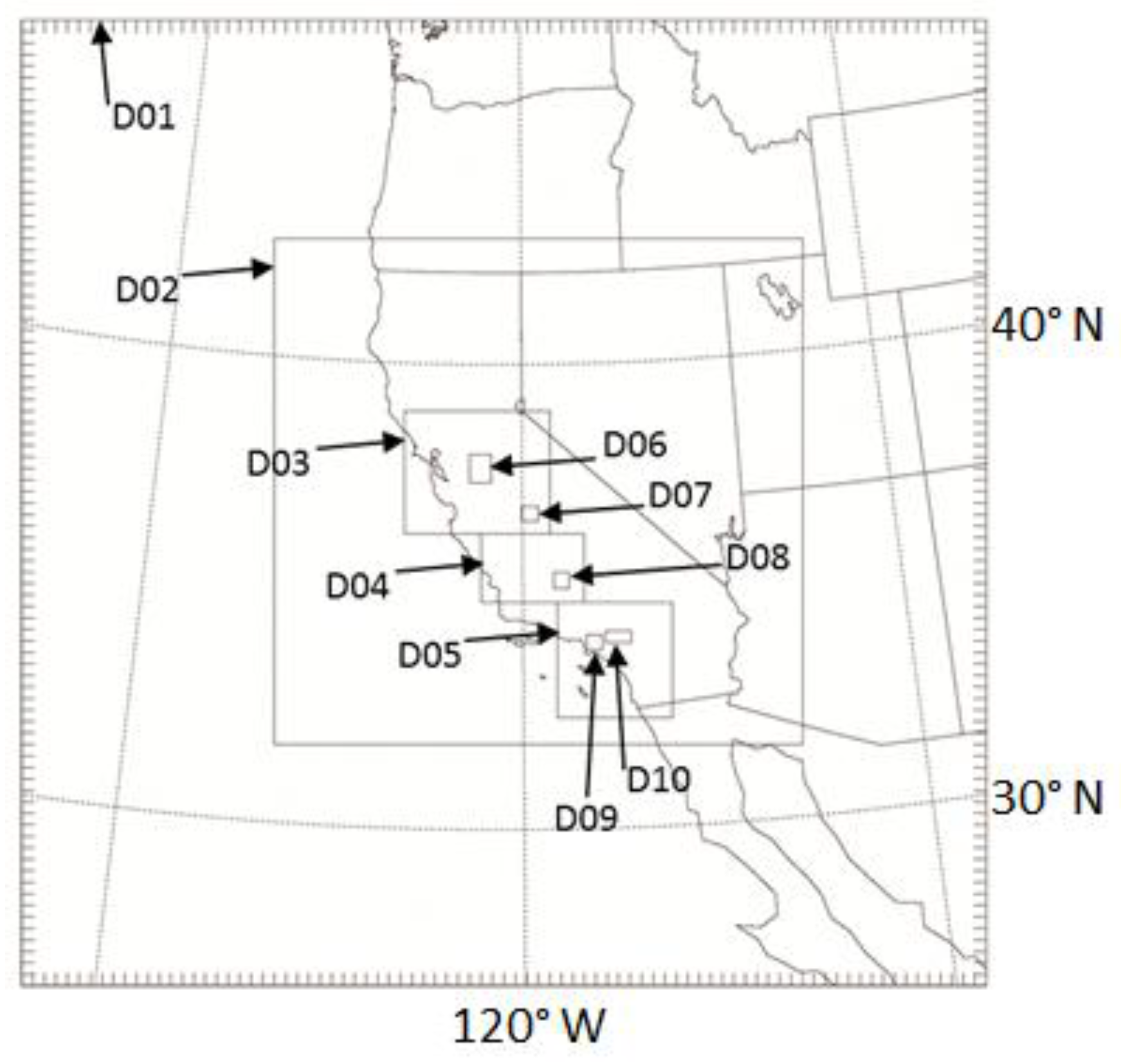
The modeling periods presented in this paper encompass the months of June, July, and August (JJA) 2013 and JJA 2006, the latter of which was employed to capture the impacts of the California heat wave of 15 July through 1st August of that year [32,33]. Figure 1 depicts the nested-grids WRF configuration used in this study. The 3- and 1-km grids were positioned in relation to the CalEnviroScreen top 20%, 10%, and 5% score areas [21], so as to focus on the regions with an increased health risk and population vulnerability. Top scores in CalEnvioScreen indicate the worst conditions in terms of public health. Thus, for example, the top 5% score is worse than 10% and so on.
2.5. Model Input
Four-dimensional NCEP-NCAR Reanalysis [34] for the years 2006 and 2013 was used for the model boundary conditions and data assimilation (FDDA). Additional NWS/NOAA datasets were obtained to complement the reanalysis, including the surface temperature, sea-surface temperature, soil moisture, and upper-air meteorology. Fine-resolution mesonet observations (e.g., NOAA/MADIS) from the areas of interest were also used in carrying out a quantitative model performance evaluation (MPE).
Land-use/land-cover (LULC): As is often the case, some California urban areas are extremely data-rich, whilst others are relatively more data-sparse. In order to ensure an even and comparable California-wide characterization, two LULC datasets were used: (1) 30-m United States Geological Survey (USGS) Level-II and Level-IV [35] classification representing years up to 2000; and (2) 30-m National Land Cover Data (NLCD) representing year 2011 [36]. While these datasets may be less resolved than other local data when available, their even statewide coverage was one main criterion for selection. A crosswalk between the two datasets was carried out [22] to increase the number of useful LULC categories. NUDAPT/WUDAPT datasets [31] were not used directly in this effort because of their limited spatial coverage, but as templates, along with local climate zones [37] to map morphological characteristics onto LULC classes.
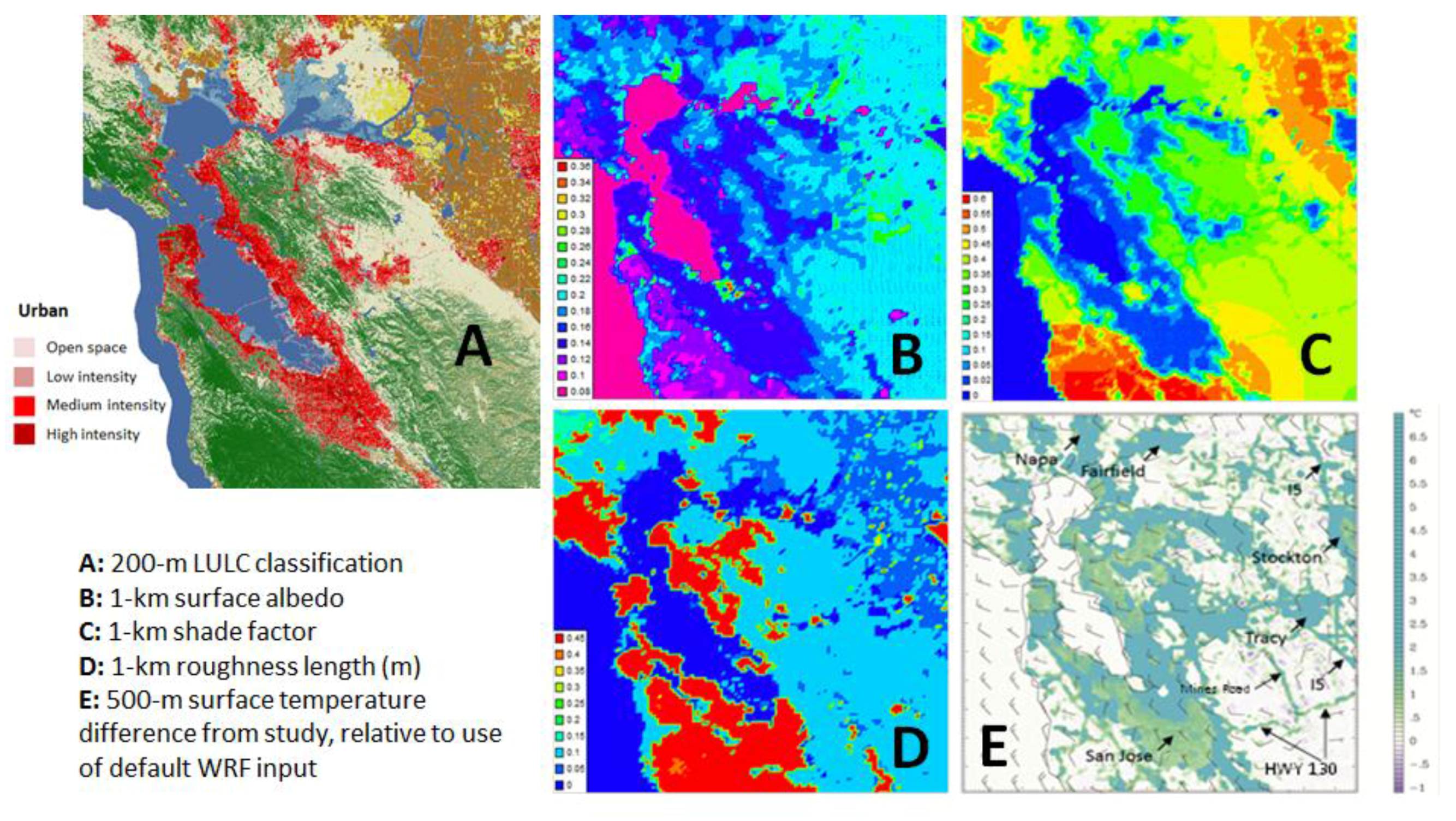
The LULC characterization of each domain provides a basis for the derivation of certain physical parameter inputs to the land-surface models. The approach in this study uses a bottom-up characterization of each model grid cell based on surface physical properties. That is, instead of scaling up the LULC classes and assigning lookup values of physical parameters to the dominant (by majority) LULC in each grid cell, as is done in the default input to WRF, this study scales up the physical properties and parameters (rather than LULC) so that details of physical characteristics are preserved. The simulation improvements gained from this approach can be seen in Figure 2 as an example (San Francisco Bay Area). The methodology is detailed in Taha and Freed, 2015 [22]—here, only some highlights are discussed.
In Figure 2A, an example LULC characterization of the San Francisco Bay Area, via NLCD 2011, is shown. The areas in red are various classes or urban LULC. Figure 2B–D present, respectively, the albedo, canopy shade factor, and roughness length derived based on the LULC characterizations from multiple datasets. In Figure 2E, surface-temperature differences between two cases are shown: (a) simulations pursued with study-specific WRF customizations and input modifications; and (b) WRF simulations with the standard input approach. The study-customized approach preserves the fine-scale urban details of relevance to UHI/UHII calculations. For example, as seen in Figure 2E, the major highways in the area (some of which are labeled on the figure), as well as detailed city boundaries, are clearly reflected in the simulated temperature pattern. Note that the temperature-difference scale in Figure 2E is intentionally selected to show two shades of green: the light green color roughly represents the areas classified as urban in standard WRF processing (temperature difference is between 0 and 1.5 °C). On the other hand, the dark-green color represents additional areas classified as urban in the modified approach (temperature difference of 2–4 °C, or more).
2.6. Model Modifications and Customizations
This study modified the process by which thermo-physical characterizations of the urban surface were carried out at various grid-nest levels for input into the land surface model in WRF (Noah LSM) and to the urban physics parameterizations discussed in Section 2.3. The goal of this modified approach was to preserve the fine-scale urban features and their effects that are important in modeling urban heat. The LULC and surface characterization is carried out independently at each grid level (for each nest). Unlike in standard WRF processing where LULC is scaled up and used in characterizing a grid cell, here the physical properties are scaled up instead, thus better preserving such properties at finer resolutions, including effective albedo, soil moisture, roughness length, canopy cover, shade factor, and urban morphometric and drag-related parameters, as discussed in Section 2.5. The basis for assigning thermo-physical properties at the surface-type level (e.g., roof, wall, street, tree level, etc.) in this project was the California urban-fabric analysis in several studies [9,18,19,38,39,40]. These aspects are discussed in Taha and Freed, 2015 [22] along with the model physics options, configurations, and parameterizations selected in this study, as well as methodologies for the computation of relevant gridded urban surface parameters.
The physical properties at urban points within each grid cell were then meshed with those of their non-urban surroundings, i.e., portions of cells that are non-urban, by weighing the respective physical properties by the fractions urbfra and 1-urbfra, where urbfra is the cell’s urban content. This is an improvement over the way in which urban and non-urban land uses within urban grid cells are characterized by default in urban WRF, where the non-urban part of an urban grid cell is typically reverted to some default category regardless of what existed in that grid cell originally. Furthermore, in implementing these modifications in the land-surface model, a distinction was made, in this study, between “above-canopy” and “below-canopy” vegetation cover [38,40]. In terms of model input parameters, the former is used in shade-factor calculations, whereas the latter is employed for adjusting the soil-moisture content.
Whereas the coarser grids were run with two-way feedback and analysis nudging FDDA, a nest-down approach was adopted for the finer grids of the configuration shown in Figure 1. In this study, nesting down to the finer domains was updated to directly ingest the output from the urban characterization steps discussed above.
2.7. UHI/UHII Reference Points
The interaction between UHI circulation and the background flow has been examined in several studies [9,41,42]. For an urban area, there is generally a certain wind-speed threshold that determines the relative dominance and impacts of background versus UHI-induced flows. This wind-speed threshold has been shown to depend on the city size, among other factors [43,44]. In this study, the dominance of background versus UHI circulation is determined hourly from the modeled fields by comparing the flow directions within and outside of each urban area.
Thus, unlike in simpler approaches where the UHI is computed relative to fixed reference point(s), this modeling study computes the UHI at each census tract relative to several time-varying (hourly) wind-dependent upwind reference points. That is, the UHI at each census tract is quantified dynamically based on the varying wind direction, such that the reference points are always upwind of the urban area. The dynamical calculations of the UHI/UHII and the criteria for selecting the reference points are discussed in Taha and Freed, 2015 [22].
Note that the combined effects of (1) time-varying reference points in calculating the UHI and (2) the inclusion of only time intervals when urban areas are warmer than non-urban reference points (see the “min” operator in Equation (1)) can result in spatial patterns of the UHI and UHII that are counter-intuitive, especially in climate archipelagos, as will be discussed in Section 3.1.
2.8. Model Performance Evaluation
As alluded to in Section 2.3, a rigorous model performance evaluation (MPE) was carried out in this study [22] and the performance was found to be satisfactory. The MPE was conducted using observational data from 151 NOAA meteorological monitors covering the fine-resolution California sub-domains (Figure 1) for periods JJA 2006 and 2013. The performance was compared against recommended benchmarks for temperature, wind speed, wind direction, and humidity, through metrics such as the forecast skill, mean bias, mean absolute error, root mean square error (including both systematic and unsystematic), index of agreement, and related variables [45]. For example, for D02, the mean wind speed bias is 0.08 m s−1, root mean square error 1.73 m s−1, and index of agreement 0.78. For wind direction, the bias is 0.92° and absolute error 35°. The temperature bias is 0.7 K, absolute error 2 K, and index of agreement 0.93. Finally, for humidity, the bias is −0.89 g kg−1, absolute error 1.47 g kg−1, and index of agreement 0.65. All of these values are well within or close to the recommended benchmarks for each variable. In addition to the statistical MPE of near-surface meteorology, a subjective evaluation of the upper-air model performance at 850, 700, and 500 hPa was undertaken to assess the model’s ability to reproduce observed synoptic-scale features.
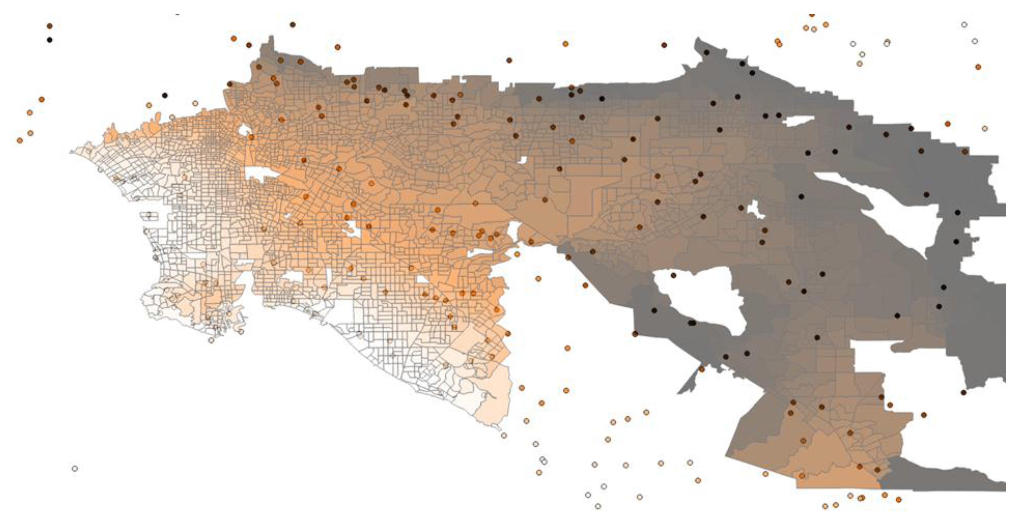
Furthermore, observations from ~1200 mesonet stations in Californian urban areas (NOAA/MADIS) were also used for a more localized MPE in the study’s domains. These observations were used in evaluating the model’s ability to reproduce fine-scale observed temperature patterns and UHI. The example in Figure 3 (for the Los Angeles region) shows that the model can capture the observed UHI, temperature gradients and spatial patterns, and the archipelago effect. In this figure, observations and simulations for the month of June 2013 are shown.
3. Results and Discussion
3.1. UHII Calculations
The UHII, as defined in Equation (1), was computed for every census tract in 40 Californian urban areas and for each hour of JJA 2013 and 2006. Among several metrics examined in the study, the cumulative totals were converted to degree-hour per day (DH/day) averages, as in Table 1. The range of DH/day (column 3) reflects the variability of the UHII within each area. Column 2 identifies regions as either an “urban island” or collection of islands (UI) resulting in single-core or multi-core UHIs, or as an “urban-climate archipelago” (UA) (see discussion in Section 3.2). Column 4 represents the temperature difference between census tracts with higher UHIIs and those with lower UHIIs within each region. This represents an all-hours averaged UHI; however, in the datasets generated in this study [22], the temperature difference at each census tract is also provided individually, not just as the maximum region-wide value, as in column 4. Of note, in calculating the temperature difference in column 4 the non-urban reference points were not used. Rather, this difference is calculated between the census tracts with the highest UHII and urban areas with the lowest UHII.
It is important to note that the UHII range (column 3) was computed independently for each area and not based on common UHI reference points across the regions. In other words, the absolute temperatures cannot be inter-compared across different areas in column 1. The UHII and temperature differences appear to be large in some instances (particularly UA regions) because they also include urban-climate archipelago effects (superimposed signals). This will be discussed further below.
In analyzing the spatial characteristics of the UHII in the 40 urban areas modeled in this study, it is possible to discern four types of spatial patterns:
- Small areas: where urban areas are relatively small and, thus, UHIs are small and localized.
- Single cores: these are relatively larger urban areas where the UHI can develop fully and the downwind transport of heat can occur. There is one core, i.e., one main area where the UHI maximum can be defined and thus a single-core UHII can be identified.
- Multiple cores: in this case, several UHI cores develop, although each core is still well defined.
- Climate archipelagos: In this situation, urban land use covers a large geographical area often demarcated by coastlines or topography (in California). Thus, unlike single- or multi-core urban areas, where there is a clear beginning and end to urban land use, urban-climate archipelagos consist of sustained built-up cover, with minimal interruption. The only discontinuities in the urban expanse usually occur because of topography. Examples include San Francisco Bay Area and the Los Angeles basin.
Examples of these different UHI and UHII patterns (i–iv) for 40 urban areas, along with the maps and related datasets that were produced in this study can be found at https://calepa.ca.gov/wp-content/uploads/sites/34/2016/10/UrbanHeat-Report-Report.pdf and https://www.calepa.ca.gov/climate/urban-heat-island-index-for-california/urban-heat-island-interactive-maps/.
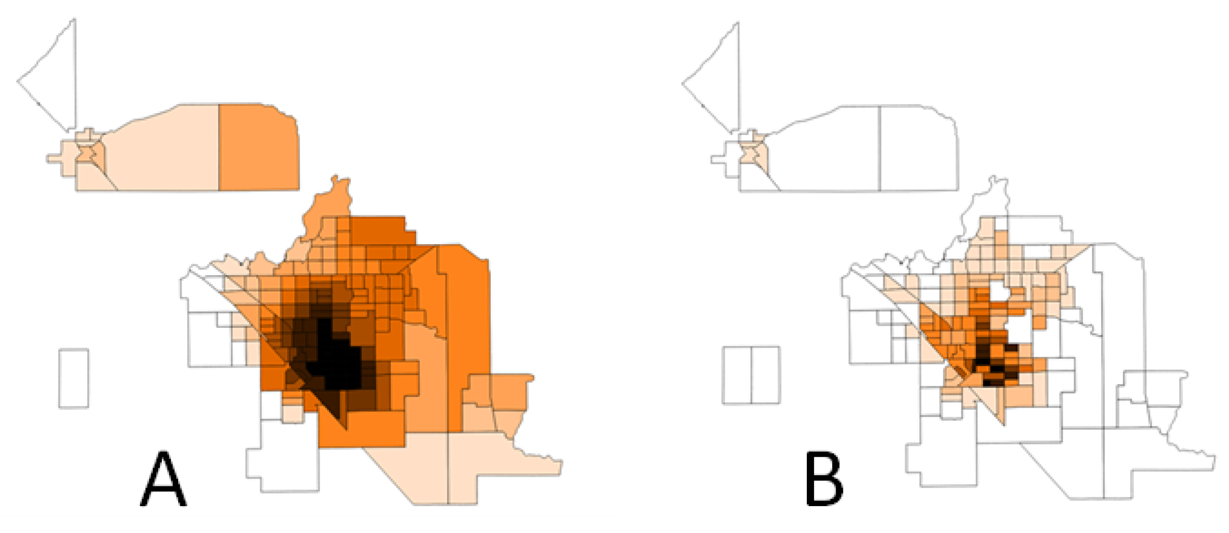
In the following discussion, an example of a single-core UHI (Fresno) and a climate archipelago (Los Angeles region) are presented (from 40 urban areas modeled in this study). These are shown in Figure 4 and Figure 5, respectively, where Figure 4A is the Fresno UHII computed as degree hours per day (DH/day) and Figure 4B is the UHII weighted by population density. Similarly, Figure 5A shows the Los Angeles area UHII (DH/day), including the climate-archipelago effect, and Figure 5B is the UHII weighted by population density at each census tract (the western half is shown and will be discussed further in Figure 6). Population density is used in this discussion as an indirect proxy to urban density. Population weighting is done by multiplying each census tract’s UHII by the ratio of its population density to that of the most populous tract in the area (highest density). Thus, the census tract with the highest population density has a weight of 1 for its UHII.
As discussed in Section 2.2, the UHI and UHII are based on 2-m air temperature, not skin-surface temperature (the latter typically results in patterns of hot and cold spots that are more familiar and similar to satellite thermal imagery). Further, the results presented here are for resolutions of 1–3 km. Therefore, the UHII calculations account for the effects of heat transport and mixing. Note that finer-scale modeling, e.g., at 500 m, shows more localized and more detailed temperature patterns, but these are not relevant to the Level-1 and Level-2 UHII characterizations presented here (and defined in Section 2.2).
Figure 4A and Figure 5A show a Level-1 UHII, whereas Figure 4B and Figure 5B show a partial Level-2 product. It should be emphasized here that the type of information provided by Level-2 UHII, such as presented in Figure 4B and Figure 5B, does not represent real-world temperature conditions like Level-1 UHII; they are only a useful tool to aid in the allocation of resources and in planning. As can be seen in these figures, the effects of the climate archipelago are evident. In the Fresno area, the population-weighted UHII spatial pattern is relatively similar to that of the UHII Level-1 (compare Figure 4A and Figure 4B). That is because the region is relatively uniform geographically and, thus, the distribution of urban heat is relatively proportional to that of the population. However, in the Los Angeles region, the population-weighted UHII pattern differs from the Level-1 pattern (compare Figure 5A and Figure 5B), because of the climate-archipelago effect and on-shore warming of the air. In this case, heat transport results in the highest temperatures in areas that are not necessarily the highest in population density.
In the Los Angeles region, the Level-2 population-weighted UHII (Figure 5B) may look more familiar and intuitive than Level-1 (Figure 5A) as the latter shows heat transport downwind throughout the climate archipelago, away from the coastline and towards the foothills and inland basin (east), and thus makes the localized variations in the UHI less noticeable and the pattern less intuitive. Among the observations that can be made with regard to Level-2 UHII in the Los Angeles region (i.e., Figure 5B relative to A) are: (1) Downtown Los Angeles (white oval) can be seen as a hotter area than its surroundings; (2) the hot areas in the north are displaced southward and away from the foothills (top part of the figure); and (3) the hotter areas in the eastern basin are more confined (not shown).
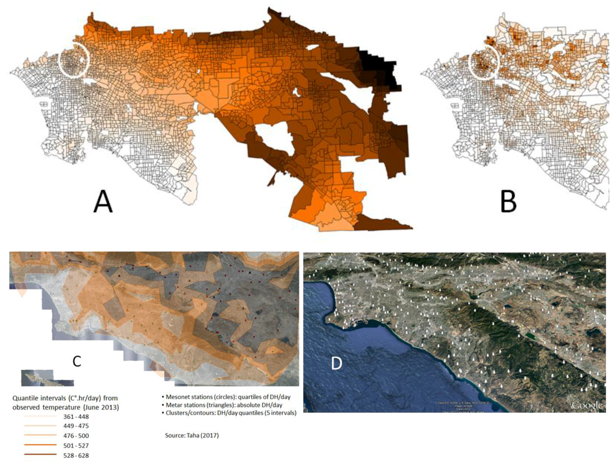
However, the UHII pattern in Figure 5A correctly reflects the actual conditions, that is, the model results are supported by observations. For example, the DH/day clustering (Figure 5C) based on the observed mesonet temperature from June 2013 clearly shows a spatial pattern and magnitudes that are similar to those from the model in Figure 5A (the clustering is done by grouping together weather stations (Figure 5D) that have similar DH/day values within given quantile intervals). Note that Figure 5A shows the UHII, i.e., differences relative to reference points, whereas Figure 5C shows the absolute DH/day at each station (not differences).
In a climate archipelago, the range of UHII is usually large and such a region, when examined at a coarse scale, appears as if uniform in UHII values over large swaths (see Figure 6 for the west Los Angeles basin discussed earlier as an example). In reality, however, the model captures localized variations (fine-scale signals) in temperatures and locally-generated UHIs at fine scales, e.g., the census tract level, throughout such a region, in addition to the dominant on-shore warming and archipelago signals, e.g., as seen in Figure 6. These superimposed signals are discussed further in Section 3.2.
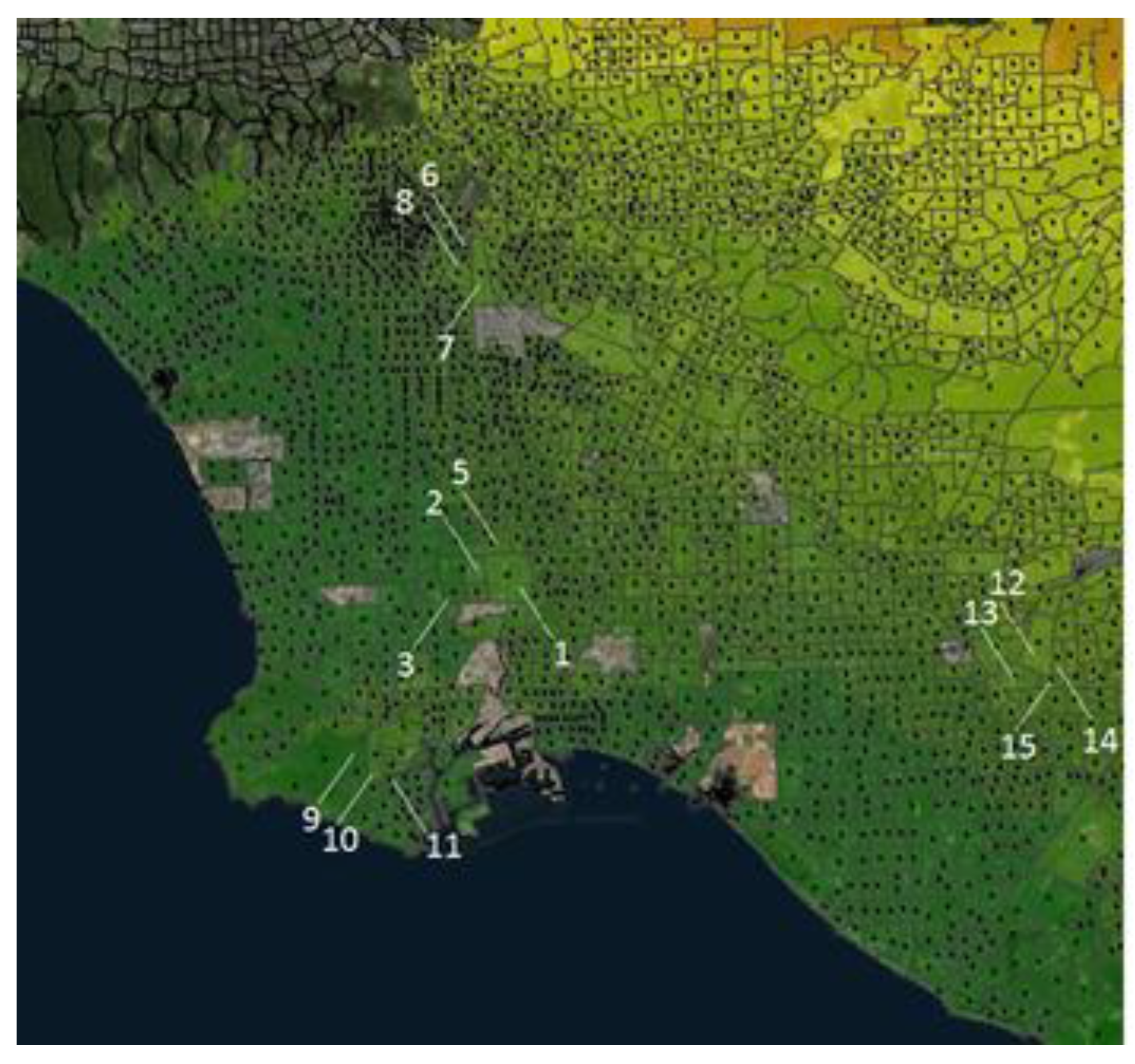
An additional analysis of the Los Angeles climate archipelago is provided here as an example. Census tracts numbered 1–5 in Figure 6 are in the Compton area, tracts numbered 6–8 are in Downtown Los Angeles, tracts 9–11 are in the San Pedro area, and tracts 12–15 are in the Anaheim-Orange area. These clusters of census tracts are also listed in Table 2 and the purpose of discussing them here is to show examples of micro-scale variations (locally-generated UHI and correlation with LULC) that are captured by the model but are embedded within the dominant signal of the climate archipelago and on-shore warming.
In the Compton area, the largest UHII is found at point 1 and the smallest at points 2 and 3. The corresponding average UHIs are 0.77, 0.54, and 0.52 °C, respectively. This represents a localized temperature difference (a locally-generated UHI) of 0.25 °C across a distance of less than 1 km. Tract 1 (with highest UHII) represents industrial-commercial land use, whereas tracts 2 and 3 (lowest UHII) represent residential land use with higher vegetation cover than in tract 1.
In Downtown Los Angeles, Financial-District census tract 6 (high-rise area of downtown) has the largest UHII among the three tracts considered. The locally-generated UHI in the high-rise area is 0.33 °C relative to tract 8 (South Park, a commercial area), which is less than 1 km to the south. The high-rise area is also similar to or slightly warmer than tract 7 (Arts District), despite the latter being (1) downwind of downtown and (2) in an industrial-commercial area.
In the San Pedro area, census tract 10 has a larger UHII than tracts to the west of it (tract 9), as well as to the east of it (tract 11). Both tracts 9 and 10 are residential; however, tract 9 has a lower density development than tract 10 and has significantly higher vegetation cover. Tract 10 is a high-density development with lower vegetation cover. As a result, tract 10 has a larger UHII than tract 9. Tract 11 is near golf courses and is cooler than tract 10. Just a few hundred meters south of tract 11, in a golf-course area, the UHII is 12.75 DH/day and is 0.5 °C cooler than tract 10.
It can also be observed that the Compton area is “counter-gradient” relative to San Pedro. In other words, whereas Compton is expected to be warmer than San Pedro, due to being further inland from the coast, it is actually cooler (thus counter gradient). It is also notable that relative to the west basin’s UHI reference points, the downtown area (tract 6), while relatively more inland, has an average UHI of 1.68 °C, whereas tract 10 has an average UHI of 1.04 °C despite being closer to the coast. This highlights the influence of land-use and land-cover properties, as well as the ability of the model to detect these fine-scale effects that are embedded within the larger-scale signals (Figure 6).
In the Anaheim-Orange area, the largest UHIIs among the four tracts examined are 46.06 DH/day in tract 12 and 45.74 DH/day in tract 14. Relative to the lowest UHII of 37.86 at tract 13, this represents a localized average temperature difference of 0.34 °C across a distance of less than 1 km. Tract 12 is industrial-commercial with lower vegetation cover than the surrounding tracts and, thus, has the highest UHII. Tract 13 is residential, with significantly larger vegetation cover and the lowest UHII in this sample area. Tract 14 is also residential and is vegetated but is downwind of tract 12, hence the larger UHII, but still slightly smaller than in tract 12. Finally, tract 15 is mixed residential and commercial land with significant vegetation cover and lower UHII.
While a number of urban-climate archipelagos have been identified world-wide [46], including, in California, both the Los Angeles Basin and the San Francisco Bay Area, quantifying their atypical UHIs is not standard procedure and not much prior guidance is available in this respect. Thus, the work performed in this study could be considered as one attempt at characterizing archipelagos in terms of UHI/UHII.
3.2. Climate Archipelagos and Air Temperatures
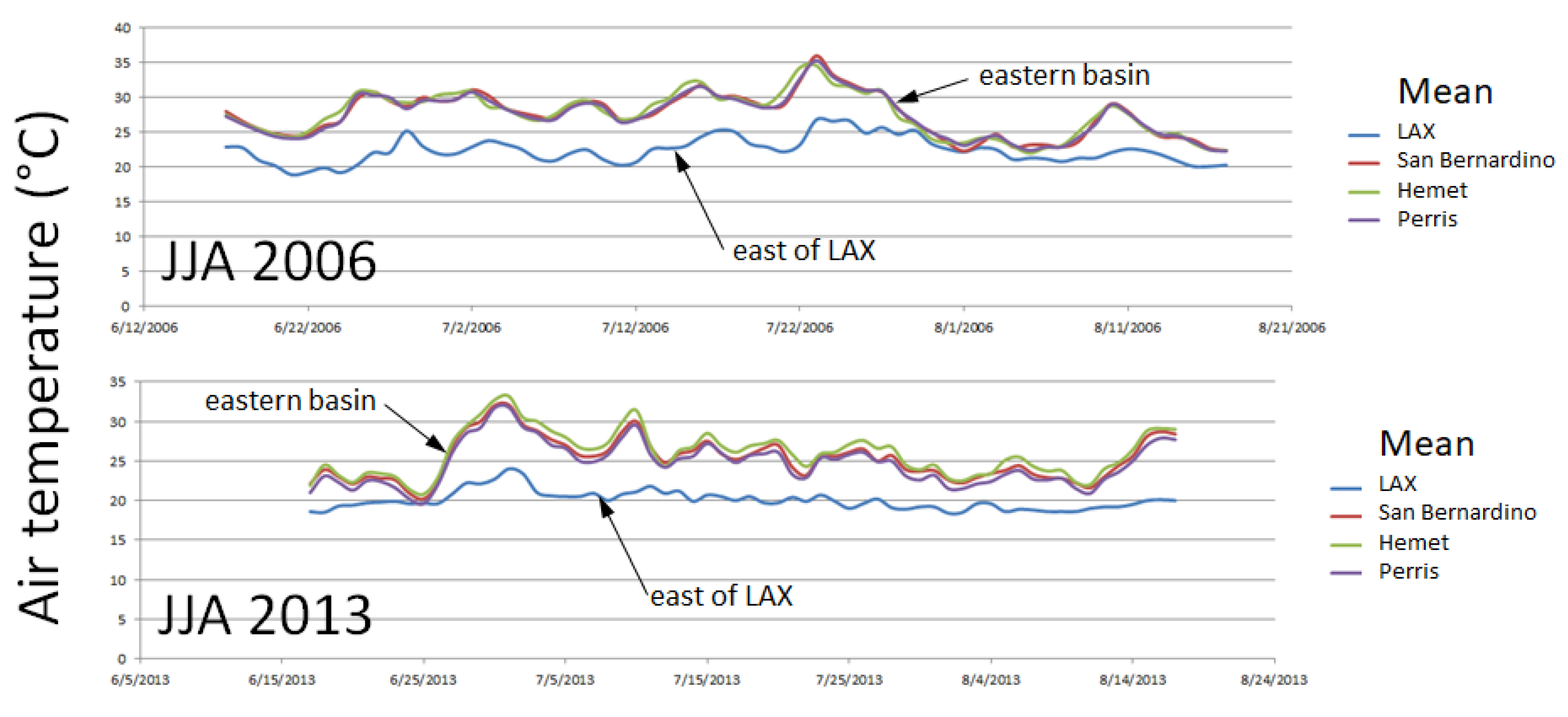
An urban-climate archipelago acts as one large area-source of heat (no distinguishable core) and the highest temperatures are typically found downwind. In the case of the Los Angeles basin, the model results indicate an average air-temperature difference of 6–8 °C between inland areas (e.g., the towns of San Bernardino, Hemet, and Perris) and coastal areas, e.g., areas to the east of Los Angeles International (LAX), as seen in Figure 5A. Observational and analyzed data from PRISM [47] suggest an average temperature difference of 5–7 °C between these regions (Figure 7). The ~1 °C shift between modeled and PRISM UHI can be attributed to the finer resolution of the modeling, as well as the locations of the actual monitors and grids (in PRISM) versus the locations of the centroids (census tracts) used in the simulations. However, the example shows a good agreement between the modeled and analyzed temperature differentials in the archipelago.
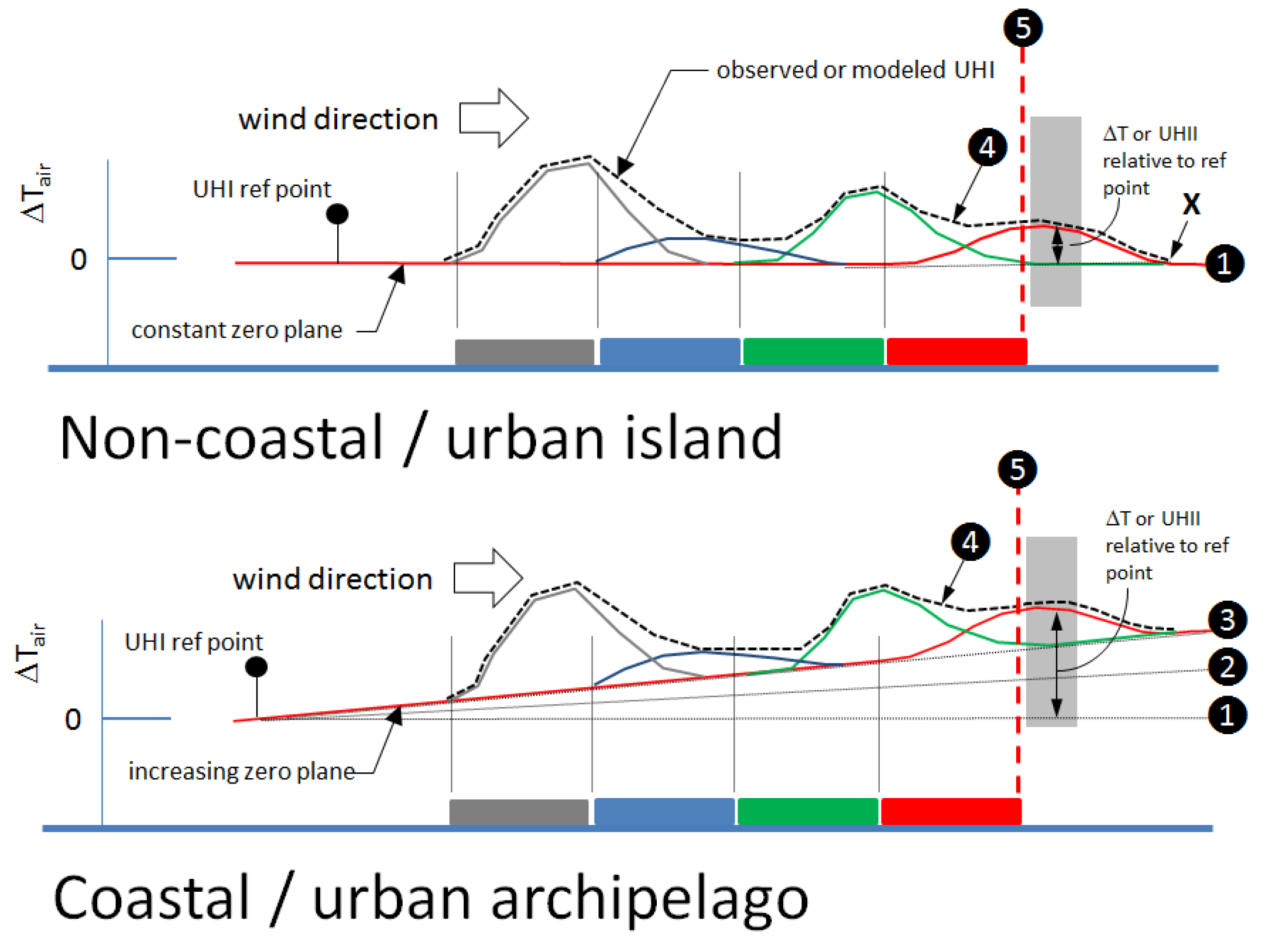
The climate-archipelago and single/multi-core UHII situations can be further explained schematically with the aid of Figure 8. Using a perturbation analogy, the UHI (∆T) at any point can be decomposed into a background component (leading up to that point) and a local component (at the point), such that:
In Figure 8, line 1 in the top graph and line 3 in the bottom graph represent the background UHI component (e.g., resulting from urban-climate archipelago effects and the on-shore heating of air), whereas the multiple colored lines (in both top and bottom graphs) represent the locally-generated UHI, that is, the deviation of the local UHI (as totalized in line 4) from the background. Line 4 represents the sum of the localized UHI and the heat transported from the urban areas upwind of it. The top figure represents a relatively smaller urban area where no archipelago effect exists and, thus, line 1 has a slope of near zero. Relative to the upwind reference temperature (UHI ref point), a “zero plane” is defined (line 1 in top graph, line 3 in bottom graph) which can serve as a reference temperature that does not include the urban-archipelago or on-shore warming effects.
In the case of an urban island (UI), as in the top graph of Figure 8, such as in Fresno (see Figure 4A), the temperature (line 4) returns to about the value of the upwind reference point, i.e., the value at the zero plane (line 1) at some distance downwind of the trailing edge of the urban area (the trailing urban edge is marked with line 5). This tapering-off of the UHI is complete at the point marked with “X” (in the top graph), where conditions are relatively similar to those upwind (i.e., at the UHI ref point) if the urban area is relatively small. At the trailing edge of the urban area (line 5) there is still a UHI, as seen by the continuous red line and the dashed black line (line 4).
In coastal and/or urban-climate archipelago situations (bottom graph of Figure 8), such as Los Angeles Basin (see Figure 5A), the zero plane (line 3) increases in the on-shore direction and the urban area (archipelago) ends at topographical barriers (thus the archipelago ends at line 5). There is no downwind stretch past this trailing edge of the urban area (to the right of line 5) over which the temperature can readjust and return to upwind values. As a result, the total UHI at that point (at line 5 in bottom graph) consists of the following superimposed fields: (a) the onshore warming of air (line 2 minus line 1); (b) upwind urban warming of air by the urban archipelago (line 3 minus line 2) beyond that caused by the local urban land use; and (c) the locally-produced UHI (line 4 minus line 3). This explains why the highest UHII values in archipelagos and coastal areas are found further inland, near the downwind end of the air basin, close to the foothills (e.g., Figure 5A). At these barriers, which also are the trailing edges of the urban archipelagos, the temperature is generally higher than in other parts (the observational data also support these findings). Thus, line 4 and line 3 in the bottom graph of Figure 8 represent what is seen in Figure 6, i.e., variations in localized UHIs superimposed on a dominant west-to-east gradient in temperature.
As a result, areas with similar local UHIs (for example in the regions highlighted with grey vertical shade in Figure 8) will have a larger UHII in archipelago situations (bottom graph) than in urban islands (top graph) because of the superimposed on-shore warming and archipelago effects in the former. Or, conversely, an area with a certain UHII in the archipelago can have a smaller localized UHI than an area of a similar UHII in an urban island situation. Note that this discussion applies only to Level-1 UHII, not Levels 2–4.
The implications are that when computing the average temperature differences (∆T) between the upwind and downwind parts of urban archipelagos/coastal areas (e.g., column 4 in Table 1), larger values are obtained than in urban islands (UI). For example, and as described earlier, the modeled ∆T across the LA basin is 6–8 °C. However, as shown in Figure 8, this ∆T, while correctly characterizing real-world conditions in this area (Figure 5A), is not solely a local UHI effect, but also includes other signals. On the other hand, for example, the average ∆T between the upwind and downwind parts in Fresno (1.9 °C) is mostly comprised of a local UHI effect, since the area is inland (no on-shore warming) and also relatively small, and thus no archipelago effect exists (flat line 1 in top graph of Figure 8). This suggests that in UI areas, the UHII is closer to being a mitigation indicator than in UA regions where it is solely a characterization of urban heat.
The cumulative urban-warming effect of an urban climate archipelago, especially in uninterrupted built-up areas like the Los Angeles basin, is a real part of the UHI and so it is correct to include it in calculating and mapping the UHII for heat-health assessments and evaluations of air quality, as was done in this study (Level-1 modeling), e.g., as shown in Figure 5A. The UHII, in this case, is proportional to what a thermometer would indicate in the field in these areas. However, the on-shore warming and archipelago effects should be subtracted in future efforts (e.g., Levels 3 and 4 modeling, as discussed in Section 2.2) if the goal is to develop localized (census-tract level) UHI mitigation guidelines or localized monitoring of the UHI at fine resolutions.
3.3. UHI Exacerbation during Hot Weather
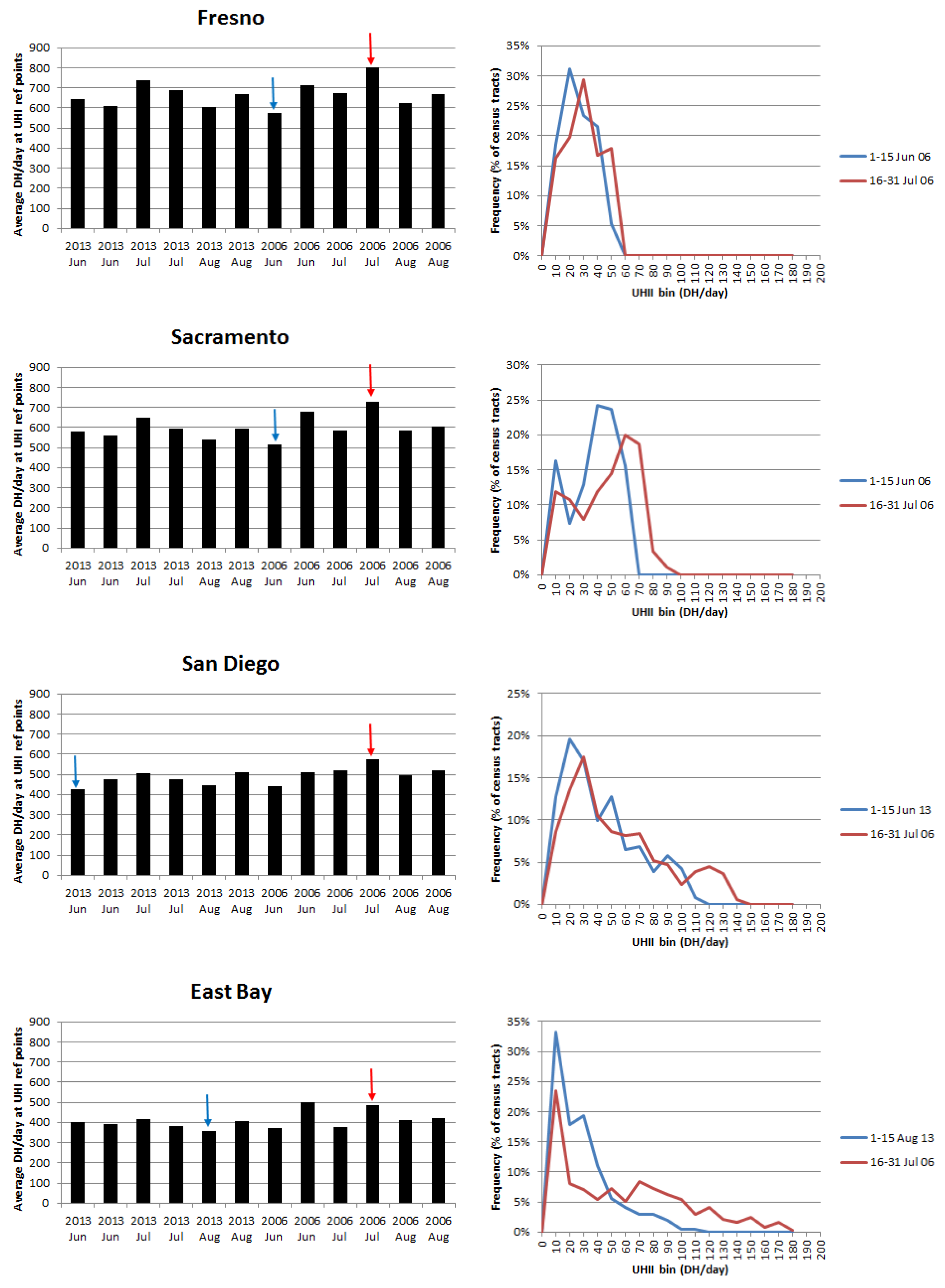
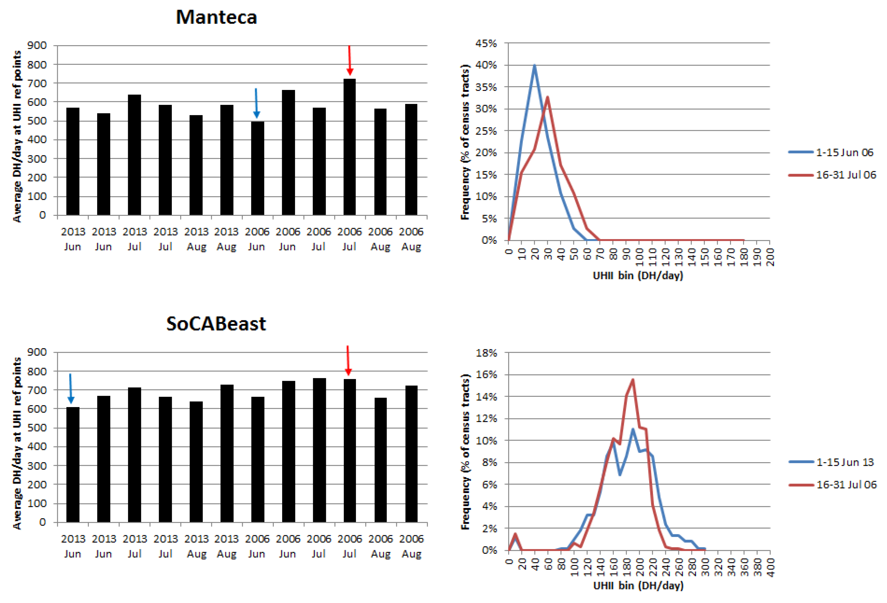
An analysis was carried out in this study to evaluate the UHII pattern in each area during hotter weather. An arbitrary sample of regions is presented in Figure 9. In the left part of each figure, the average UHII (DH/day) for each region’s reference points is shown for the JJA periods in 2013 and 2006 and used here as a cumulative indicator to and in lieu of the instantaneous absolute air temperature. The 2006 heat wave is marked with red arrows.
On the right side of each figure, two frequency distributions are shown: one for the 2006 heat wave (red line, corresponding to red arrow) and another for the period with the lowest average UHII in each region (blue line, corresponding to blue arrow). In the right part of the figures, the horizontal axis represents the UHII (in bins of 10 DH/day) and the vertical axis is the frequency, i.e., the percentage of census tracts within given UHII bins. Of note, each of the cooler and heat-wave periods are two weeks long and the coolest periods differ across the regions (blue arrows).
It can be seen in Figure 9 that the warmer weather shifts the UHII distribution towards larger values compared to the cooler periods. For example in Fresno, about 30% of census tracts in the UHII bin of 20 DH/day are shifted to the 30 DH/day bin. The 50 DH/day bin initially containing 5% of tracts in the cooler weather contains 18% of the tracts during the heat wave.
In Livermore (not shown in Figure 9), the 40 DH/day bin contained 14% of tracts during the cooler period, but 22% during the heat wave. This was shifted from the lower bin of 30 DH/day which contained 24% of tracts in cooler weather but decreased to 17% of tracts during the heat wave. In Sacramento (Figure 9), significant shifts occur such that the bin at 70 DH/day contained 0% of tracts during the cooler period but increased to 19% of tracts during the heat wave. The distribution of tracts in other bins also changed with some increasing and others decreasing.
In San Diego (Figure 9), the shift occurs through a range of bins, but noticeably, the number of tracts in the 20 DH/day bin is reduced and shifted to the higher bins. Those bins of 110–140 DH/day contained 0% census tracts in the cooler period that increased to 4% of the tracts (in each of these bins) during the heat wave. In San Francisco (not shown), the census tracts in bin 10 DH/day were reduced from 72% to 54% and shifted to higher bins, such that the bins 110–180 DH/day, containing 1% of tracts during the cooler periods, increased to 3–5% of the tracts during the heat wave. In Vallejo (not shown), census tracts in bins 40–60 DH/day were shifted to bins 70 and 80 DH/day, and the bins 90–120 DH/day that contained 0% of the tracts in the cooler period increased to 8–18% of the tracts during the heat wave.
In Antioch (not shown), bins were shifted upwards such that bin 50 DH/day, containing 0% of tracts during the cooler weather, contained 14% of tracts during the heat wave. In the East Bay (Figure 9), all bins smaller than 50 DH/day were shifted to bins higher than 50 DH/day. Furthermore, bins 120–170 DH/day containing 0% of tracts during cooler periods increased to contain 2–4% of the tracts in heat-wave conditions. In Fairfield (not shown), most tracts in the 10 DH/day bin were shifted to the 20 DH/day bin during the heat event. In addition, bins 90–140 DH/day with 0% tracts in cooler weather, increased so as to contain 2–6% of the tracts during heat wave conditions. In Manteca (Figure 9), tracts in bins 10 and 20 DH/day were shifted to higher bins, such that bins 30–60 DH/day contained larger numbers of census tracts under the heat wave conditions. Significant changes and shifts in the UHII are also seen in other regions throughout California and are discussed in Taha and Freed, 2015 [22].
In the Los Angeles urban-climate archipelago, the hotter weather also increases the number of census tracts affected by a high UHII, but the pattern is different from those in the regions discussed above. For example, in east Los Angeles basin (Figure 9, SoCABeast), the heat wave causes an increase in the number of census tracts in the mid-range bins of 150–210 DH/day, but a decrease in census tracts at both tail ends of the main distribution (the smaller distribution between 0 and 20 DH/day does not change). The number of census tracts in bins greater than 210 DH/day and in those bins smaller than 120 DH/day is reduced, such that the frequency distribution has a slightly smaller spread. That is, the archipelago now has a slightly more uniform temperature field (a smaller temperature differential across the basin). Revisiting Figure 7, one can see that the observational / analyzed data also suggest a smaller temperature differential around the heat-wave period (late July through early August 2006), thus lending further credibility to the modeled results, i.e., the smaller temperature differentials shown in Figure 9 (SoCABeast).
This reduction in the higher UHII values in the Los Angeles archipelago can be attributed to an effect akin to “reverse coastal cooling”, a term coined by Bornstein and co-workers [48]. This occurs when inland areas, particularly deep basins with large catchment areas, warm up (e.g., during heat waves) and strengthen the sea breeze. The stronger venting, in turn, decreases the temperature differential across the archipelago or basin. A similar effect is also seen in Santa Clara Valley in the San Francisco Bay Area. Prior studies have identified and quantified a reverse coastal cooling effect albeit on longer time scales [48] in both the Los Angeles Basin and the San Francisco Bay Area. Similarly, a more recent study of Texas [49] found that warming caused by climate change has increased venting in the Houston region.
In this UHII study, however, it is not being suggested that the area becomes cooler (the absolute temperatures actually become predominantly higher during the heat wave), but that the temperature becomes slightly more uniform across the archipelago/basin, that is, a smaller temperature differential now exists across the region because of the relatively stronger venting. While this may only be a non-dominant, temporary mechanism, it can still affect the shape of the frequency distributions in these coastal areas.
The results discussed above suggest that the warmer weather can increase the UHI and shifts the UHII to larger values because of (1) reduced winds and mixing under high pressure systems, except in coastal basins to some extent; (2) a lower urban moisture content than in non-urban areas, which under such conditions allows urban areas to warm up more; and (3) reduced cloudiness and increased solar radiation at the surface [8,9,50].
Larger UHIs in warmer weather have also been reported in other regions [8]. For example, Li and Bou-Zeid, 2013 [51] used observational data from Baltimore, MD, to show that heat waves increase the UHI intensity. Their data demonstrate that the 2008 heat wave increased the nighttime UHI from 0.5 to 2.5°C and the daytime UHI from 0.25 to 1.5°C. Li et al., 2015 [52] also use observational data from China to show that heat waves increase the UHI. Thus if warmer weather increases the UHI, then mitigation measures such as cool cities will become more important in the future [53], when heat waves are expected to occur more frequently. On the other hand, some studies suggest that UHIs could decrease with higher background temperatures in the long term [54]. Thus, again, this highlights the region-specific nature of urban climates and heat-island responses to changes in background weather and synoptic conditions.
While the meteorological model performance was thoroughly evaluated (as discussed in Section 2.8) and found to be satisfactory, there is no direct way to compare the model UHII to morbidity/mortality information at the fine resolutions presented in this paper. Such an effort may be undertaken in the future, but at this time, only some coarse-scale and qualitative assessments could be made. It is also important to recognize that the relationship between temperature, apparent temperature, and mortality is not a simple one: it is non-linear in nature and depends on a host of compounding factors, in addition to meteorology. As discussed earlier, the goal of developing the UHII is to provide an additional layer of information in decision-making tools such as CalEnviroScreen. In the following example, the binned UHII is compared to average daily deaths in four counties that were studied by Ostro et al., 2009 [25]. Both the model UHII and mortality data discussed here are for July 2006 which includes the heat wave period in the second half of the month.
Table 3 shows side by side the weighted UHII (wUHII) and mortality in those four counties. Note that the average daily deaths provided here are from all causes, not just heat, but since these occurred during the heat-wave month, it is plausible that a significant component is heat-related. The UHII is weighted by census tracts to make it more comparable to the total average deaths in each county (the number of tracts being a proxy to population). The weighted UHII (wUHII) is:
where B is the total number of UHII bins (in a region) in increments of 10 DH/day, tTRACT is the number of census tracts (in a region) that fall in UHII bin “b”, and dhpd is the number of DH/day in bin “b”. It can be gleaned from Table 3 that the directionality of the wUHII and the average daily deaths are similar. However, no attempt will be made here to develop any correlation on this basis alone.
4. Conclusions and Future Research
Atmospheric modeling was performed in this study for the purpose of characterizing the UHI under present climate conditions and quantifying the UHII for California, including the superimposed effects of onshore warming and urban-climate archipelagos where they occur. The study identifies various patterns of UHI/UHII including single-core, multi-core, and urban-climate archipelago UHIs. The analysis shows that the UHII is shifted to larger values under the conditions of warmer weather. Thus, the potentially more frequent occurrences of heat waves in future climates could enhance UHIs and further exacerbate the health effects of hot weather.
From this perspective, it is important to continue research in (1) evaluating and quantifying the synergies between background weather, urban climates, and heat islands; (2) quantifying the potential exacerbation of UHIs by regional climate change; (3) evaluating the implications in terms of heat- and air-quality health; and (4) assessing the potential of mitigation measures (such as cool cities) in offsetting some or all of these negative effects, and evaluating the added importance of such measures in future years.
Acknowledgments
This paper is based on work that was supported by the California Environmental Protection Agency (Cal/EPA). The statements and conclusions in this paper are those of the author and do not necessarily reflect the views of the Cal/EPA. The mention of commercial products, their source, or their use in connection with material reported herein is not to be construed as actual or implied endorsement of such products. Spatial Informatics Group is acknowledged for GIS work in prior stages of this effort.
Conflicts of Interest
The authors declare no conflict of interest.
References
- Goggins, W.B.; Chan, E.Y.Y.; Ng, E.; Ren, C.; Chen, L. Effect modification of the association between short-term meteorological factors and mortality by urban heat islands in Hong Kong. PLoS ONE 2012, 7, e38551. [Google Scholar] [CrossRef] [PubMed]
- Adachi, S.A.; Kimura, F.; Kusaka, H.; Inoue, T.; Ueda, H. Comparison of the impact of global climate changes and urbanization on summertime future climate in the Tokyo metropolitan area. J. Appl. Meteorol. Climatol. 2012, 51, 1441–1454. [Google Scholar] [CrossRef]
- Tan, J.; Zheng, Y.; Tang, X.; Guo, C.; Li, L.; Song, G.; Zhen, X.; Yuan, D.; Kalkstein, A.J.; Li, F. The urban heat island and its impact on heat waves and human health in Shanghai. Int. J. Biometeorol. 2010, 54, 75–84. [Google Scholar] [CrossRef] [PubMed]
- Taha, H. Potential Impacts of Climate Change on Tropospheric Ozone in California: A Preliminary Assessment of the Los Angeles Basin and the Sacramento Valley; Lawrence Berkeley National Laboratory Report LBNL-46695; Lawrence Berkeley National Laboratory: Berkeley, CA, USA, 2001; Available online: http://escholarship.org/uc/item/5s41x609 (accessed on 3 March 2016).
- Potchter, O.; Ben-Shalom, H.O. Urban warming and global warming: Combined effect on thermal discomfort in the desert city of Beer Sheva, Israel. J. Arid Environ. 2013, 98, 113–122. [Google Scholar] [CrossRef]
- Vanos, J.K.; Cakmak, S.; Kalkstein, L.S.; Yagouti, A. Association of weather and air pollution interactions on daily mortality in 12 Canadian cities. Air Qual. Atmos. Health 2014, 8, 307–320. [Google Scholar] [CrossRef] [PubMed]
- Kalkstein, L.; Sailor, D.; Shickman, K.; Sherdian, S.; Vanos, J. Assessing the Health Impacts of Urban Heat Island Reduction Strategies in the District of Columbia; Report DDOE ID#2013-10-OPS; Global Cool Cities Alliance: Washington, DC, USA, 2013. [Google Scholar]
- Taha, H. Cool cities: Counteracting potential climate change and its health impacts. Curr. Clim. Chang. Rep. 2015, 1, 163–175. [Google Scholar] [CrossRef]
- Taha, H. Meso-urban meteorological and photochemical modeling of heat island mitigation. Atmos. Environ. 2008, 42, 8795–8809. [Google Scholar] [CrossRef]
- Taha, H. Meteorological, emissions, and air-quality modeling of heat-island mitigation: Recent findings for California, USA. Int. J. Low Carbon Technol. 2013, 10, 3–14. [Google Scholar] [CrossRef]
- Taha, H. Meteorological, air-quality, and emission-equivalence impacts of urban heat island control in California. Sustain. Cities Soc. 2015, 19, 207–221. [Google Scholar] [CrossRef]
- Papanastasiou, D.K.; Melas, D.; Kambezidis, H.D. Air quality and thermal comfort levels under extreme hot weather. Atmos. Res. 2015, 251, 4–13. [Google Scholar] [CrossRef]
- Wang, X.; Chen, F.; Wu, Z.; Zhang, M.; Tewari, M.; Guenther, A.; Guenther, A.; Wiedinmyer, C. Impacts of weather conditions modified by urban expansion on surface ozone: Comparison between the Pearl River Delta and Yangtze River Delta regions. Adv. Atmos. Sci. 2009, 26, 962–972. [Google Scholar] [CrossRef]
- Lombardo, M.A. Ilhas de Calor nas Metropoles: O Example de Sao Paulo; Editora Hucitec: Sao Paulo, Brazil, 1985; p. 244. [Google Scholar]
- Rajagopalan, P.; Lim, K.C.; Jamei, E. Urban heat island and wind flow characteristics of a tropical city. Sol. Energy 2014, 107, 159–170. [Google Scholar] [CrossRef]
- Santamouris, M. Cooling the cities—A review of reflective and green roof mitigation technologies to fight heat island and improve comfort in urban environments. Sol. Energy 2014, 103, 682–703. [Google Scholar] [CrossRef]
- Skoulika, F.; Santamouris, M.; Kolokotsa, D.; Boemia, N. On the thermal characteristics and the mitigation potential of a medium size urban park in Athens, Greece. Landsc. Urban Plan. 2013, 123, 73–86. [Google Scholar] [CrossRef]
- Taha, H. Episodic performance and sensitivity of the urbanized MM5 (uMM5) to perturbations in surface properties in Houston TX. Bound.-Layer Meteorol. 2008, 127, 193–218. [Google Scholar] [CrossRef]
- Taha, H. Urban surface modification as a potential ozone air-quality improvement strategy in California: A mesoscale modeling study. Bound.-Layer Meteorol. 2008, 127, 219–239. [Google Scholar] [CrossRef]
- Taha, H. Multi-Episodic and Seasonal Meteorological, Air-Quality, and Emission-Equivalence Impacts of Heat-Island Control and Evaluation of the Potential Atmospheric Effects of Urban Solar Photovoltaic Arrays; PIER Environmental Research Program; California Energy Commission: Sacramento, CA, USA, 2013. Available online: http://www.energy.ca.gov/2013publications/CEC-500-2013-061/CEC-500-2013-061.pdf (accessed on 3 March 2016).
- OEHHA 2014. California Communities Environmental Health Screening Tool; version 2.0 (CalEnviroScreen 2.0) Guidance and Screening Tool; Office of Environmental Health Hazard Assessment Report; Office of Environmental Health Hazard Assessment: Sacramento, CA, USA, 2014; p. 136. Available online: https://oehha.ca.gov/media/CES20FinalReportUpdateOct2014.pdf (accessed on 3 March 2017).
- Taha, H.; Freed, T. Creating and Mapping an Urban Heat Island Index for California; Report prepared by Altostratus Inc., Contract 13-001; California Environmental Protection Agency (Cal/EPA): Sacramento, CA, USA, 2015; Available online: https://calepa.ca.gov/wp-content/uploads/sites/34/2016/10/UrbanHeat-Report-Report.pdf and https://www.calepa.ca.gov/climate/urban-heat-island-index-for-california/urban-heat-island-interactive-maps/; (accessed on 3 March 2017).
- National Oceanic and Atmospheric Administration (NOAA). State Annual and Seasonal Time Series. 2017. Available online: www.ncdc.noaa.gov/temp-and-precip/state-temps/ (accessed on 1 January 2016).
- Knowlton, K.; Rotkin-Ellma, M.; King, G.; Margolis, H.G.; Smith, D.; Solomon, G.; Trent, R.; English, P. The 2006 California heat wave: Impacts on hospitalizations and emergency departments visits. Environ. Health Perspect. 2009, 117, 61. [Google Scholar] [CrossRef] [PubMed]
- Ostro, B.D.; Roth, L.A.; Green, R.S.; Basu, R. Estimating the mortality effect of the July 2006 California heat wave. Environ. Res. 2009, 109, 614–619. [Google Scholar] [CrossRef]
- Powers, G.; Huang, X.Y.; Klemp, B.; Skamarock, C.; Dudhia, J.; Gill, O.; Duda, G.; Barker, D.; Wang, W. A Description of the Advanced Research WRF; NCAR Technical Note NCAR/TN-475+STR; National Center for Atmospheric Research: Boulder, CO, USA, 2008. [Google Scholar]
- Kusaka, H.; Kondo, H.; Kikegawa, Y.; Kimura, F. A simple single-layer urban canopy model for atmospheric models: Comparison with multi-layer and slab models. Bound.-Layer Meteorol. 2001, 101, 329–358. [Google Scholar] [CrossRef]
- Chen, F.; Kusaka, H.; Bornstein, R.; Ching, J.; Grimmond, C.S.B.; Grossman-Clarke, S.; Loridan, T.; Manning, K.; Martilli, A.; Miao, S.; et al. The integrated WRF/urban modeling system: Development, evaluation, and applications to urban environmental problems. Int. J. Climatol. 2010, 31, 273–288. [Google Scholar] [CrossRef]
- Salamanca, F.; Martilli, A.; Tewari, M.; Chen, F. A study of the urban boundary layer using different urban parameterizations and high-resolution urban canopy parameters with WRF. J. Appl. Meteorol. Climatol. 2011, 50, 1107–1128. [Google Scholar] [CrossRef]
- Bougeault, P.; Lacarrere, P. Parameterization of orography-induced turbulence in a mesobeta-scale model. Mon. Weather Rev. 1989, 117, 1872–1890. [Google Scholar] [CrossRef]
- Ching, J.; Brown, M.; Burian, S.; Chen, F.; Cionco, R.; Hanna, A.; Hultgren, T.; McPherson, T.; Sailor, D.; Taha, H.; et al. National urban database and access portal tool, NUDAPT. Bull. Am. Meteorol. Soc. 2009, 90, 1157. [Google Scholar] [CrossRef]
- Trent, R.B. Review of July 2006 Heat Wave Related Fatalities in California; California Department of Health Services: Sacramento, CA, USA, 2007. Available online: http://www.cdph.ca.gov/HealthInfo/injviosaf/Documents/HeatPlanAssessment-EPIC.pdf (accessed on 3 March 2016).
- Gershunov, A.; Cayan, D.R.; Iacobellis, S.F. The great 2006 heat wave over California and Nevada: Signal of an increasing trend. J. Clim. 2009, 22, 6181–6203. [Google Scholar] [CrossRef]
- Kistler, R.; Kalnay, E.; Collins, W.; Saha, S.; White, G.; Woollen, J.; Kalnay, E.; Chelliah, M.; Ebisuzaki, W.; Kanamitsu, M.; et al. The NCEP-NCAR 50-year reanalysis: Monthly means CDROM and documentation. Bull. Am. Meteorol. Soc. 2001, 82, 247–267. [Google Scholar] [CrossRef]
- Anderson, J.R.; Hardy, E.E.; Roach, J.T.; Witmer, R.E. A Land Use and Land Cover Classification System for Use with Remote Sensor Data; USGS Professional Paper 964; U.S. Government Printing Office: Washington, DC, USA, 2001.
- Multi-Resolution Land-Characteristics Consortium (MRLC). National Land Cover Databases. Available online: http://www.mrlc.gov/nlcd2006.php (accessed on 1 January 2016).
- Stewart, I.D.; Oke, T.R. Local climate zones for urban temperature studies. Bull. Am. Meteorol. Soc. 2012, 93, 1879–1900. [Google Scholar] [CrossRef]
- Akbari, H.; Rose, S.; Taha, H. Characterizing the Fabric of the Urban Environment: A Case Study of Sacramento, California; Lawrence Berkeley National Laboratory Report LBNL-44688; Lawrence Berkeley National Laboratory: Berkeley, CA, USA, 1999. [Google Scholar]
- Rose, S.; Akbari, H.; Taha, H. Characterizing the Fabric of the Urban Environment: A Case Study of Greater Houston, Texas; Lawrence Berkeley National Laboratory Report LBNL-51448; Lawrence Berkeley National Laboratory: Berkeley, CA, USA, 2003. [Google Scholar]
- Taha, H. Urban Surface Modification as a Potential Ozone Air-Quality Improvement Strategy in California—Phase 2: Fine-Resolution Meteorological and Photochemical Modeling of Urban Heat Islands; PIER Environmental Research; California Energy Commission: Sacramento, CA, USA, 2007. Available online: http://www.energy.ca.gov/2009publications/CEC-500-2009-071/CEC-500-2009-071.PDF (accessed on 4 April 2015).
- Boucouvala, D.; Bornstein, D. Analysis of transport patterns during an SCOS97 NARSTO episode. Atmos. Environ. 2003, 37, 73–94. [Google Scholar] [CrossRef]
- Kim, Y.-H.; Baik, J.-J. Spatial and temporal structure of the urban heat island in Seoul. J. Appl. Meteorol. 2005, 44, 591–605. [Google Scholar] [CrossRef]
- Oke, T.R.; Hannell, F.G. Urban Climates. WMO Tech. Note 1970, 108, 113–126. [Google Scholar]
- Oke, T.R. City size and the urban heat island. Atmos. Environ. 1973, 7, 769–779. [Google Scholar] [CrossRef]
- Tesche, T.W.; McNally, D.E.; Emery, C.A.; Tai, E. Evaluation of the MM5 Model over the Midwestern U.S. for Three 8-Hour Oxidant Episodes, Prepared for the Kansas City Ozone Technical Workgroup; Alpine Geophysics LLC and Environ Corp.: San Rafael, CA, USA, 2001; p. 23. [Google Scholar]
- Shepherd, J.M.; Bounoua, L.; Mitra, C. Urban Climate Archipelagos: A New Framework for Urban Impacts on Climate; Earthzine: New York, NY, USA, 2013; Available online: http://earthzine.org/2013/11/29/urban-climate-archipelagos-a-new-framework-for-urban-impacts-on-climate/ (accessed on 3 March 2016).
- Daly, C.; Halbleib, M.; Smith, J.I.; Gibson, W.P.; Doggett, M.K.; Taylor, G.H.; Vurtis, J.; Pasteris, P.P. Physiographically sensitive mapping of climatological temperature and precipitation across the conterminous United States. Int. J. Climatol. 2008, 28, 2031–2064. [Google Scholar] [CrossRef]
- Lebassi-Habtezion, B.; Gonzalez, J.; Bornstein, R.D. Modeled large-scale warming impacts on summer California coastal-cooling trends. J. Geophys. Res. 2011, 116, D20. [Google Scholar] [CrossRef]
- Liu, L.; Talbot, R.; Lan, X. Influence of climate change and meteorological factors on Houston’s air pollution: Ozone case study. Atmosphere 2015, 6, 623. [Google Scholar] [CrossRef]
- Taha, H.; Wilkinson, J.; Bornstein, R. Urban Forest for Clean Air Demonstration in the Sacramento Federal Non-Attainment Area: Atmospheric Modeling in Support of a Voluntary Control Strategy; Sacramento Metropolitan Air Quality Management District (SMAQMD): Sacramento, CA, USA, 2011. [Google Scholar]
- Li, D.; Bou-Zeid, E. Synergistic interactions between urban heat islands and heat waves: The impact in cities is larger than the sum of its parts. J. Appl. Meteorol. Climatol. 2013, 52, 2051–2064. [Google Scholar] [CrossRef]
- Li, D.; Sun, T.; Liu, M.; Yang, L.; Wang, L.; Gao, Z. Contrasting responses of urban and rural surface energy budgets to heat waves explain synergies between urban heat islands and heat waves. Environ. Res. Lett. 2015, 10, 054009. [Google Scholar] [CrossRef]
- Georgescu, M.; Morefield, P.E.; Bierwage, B.G.; Weaver, C.P. Urban adaptation can roll back warming of emerging metropolitan regions. Proc. Natl. Acad. Sci. USA 2014, 111, 2909–2914. [Google Scholar] [CrossRef] [PubMed]
- Lemonsu, A.; Kounkou-Arnaud, R.; Desplat, J.; Salagnac, J.-L.; Masson, V. Evolution of the Parisian urban climate under a global changing climate. Clim. Chang. 2013, 116, 679–692. [Google Scholar] [CrossRef]
Figure 1.
Modeling domains configuration: domain D01: 27-km resolution; D02: 9 km; D03–D05: 3 km; D06 through D10: 1 km. Domain D02 is centered on California and domains D03–D10 are positioned over various parts of the state.
Figure 1.
Modeling domains configuration: domain D01: 27-km resolution; D02: 9 km; D03–D05: 3 km; D06 through D10: 1 km. Domain D02 is centered on California and domains D03–D10 are positioned over various parts of the state.

Figure 2.
Example analysis for the San Francisco Bay Area (subdomain of D03). (A) NLCD 2011; (E) WRF-simulated surface temperature difference at 1400 PDT, 15 June 2013.
Figure 2.
Example analysis for the San Francisco Bay Area (subdomain of D03). (A) NLCD 2011; (E) WRF-simulated surface temperature difference at 1400 PDT, 15 June 2013.

Figure 3.
Los Angeles region model UHII (background) and mesonet observation (small circles) at 320 stations in this domain for June 2013. Both model UHII and observations are in DH/day (°C.h/day). Lightest color is 6 °C.hr/day; darkest color is 190 °C.hr/day. Compare the color changes of the small circles (mesonet observations) with those of the background UHII which shows a good agreement between the two.

Figure 4.
Fresno UHII as the difference from reference points. Lightest color is 2 DH/day; darkest color is 45 DH/day (°C.hr/day). (A): UHII; (B) UHII weighted by population density. Fresno is an example of a conventional, single-core UHI, as defined in item ii above. The geographical area shown in this figure is located in domain D07 in Figure 1.

Figure 5.
Los Angeles area UHII as the difference from reference points, showing the climate-archipelago effect. Lightest color is 6 DH/day; darkest color is 190 DH/day (°C.hr/day). (A) UHII; (B) UHII weighted by population density; (C) clustering of observations-based DH/day (absolute) at each monitor for June 2013; (D) locations of 329 monitors in the region (basis for 4C). The Los Angeles area is an example of the urban-climate archipelago as defined in item iv, above, that also includes fine-scale superimposed microclimate signals (see Figure 6). The geographical area shown in this figure is located in domain D05 in Figure 1, and further enhanced by D09 and D10.

Figure 6.
UHII in west Los Angeles Basin. Numbers indicate example census tracts listed in Table 2 and discussed in this section.
Figure 6.
UHII in west Los Angeles Basin. Numbers indicate example census tracts listed in Table 2 and discussed in this section.

Figure 7.
(Top) 2006; (bottom) 2013. Air temperatures at inland and coastal locations in the Los Angeles region based on PRISM data [47]. See text for discussion.
Figure 7.
(Top) 2006; (bottom) 2013. Air temperatures at inland and coastal locations in the Los Angeles region based on PRISM data [47]. See text for discussion.

Figure 8.
Single/multi core UHI versus climate archipelago. The colored blocks represent different urban land uses and land covers and the similarly-colored lines represent the temperature (localized UHI) corresponding to each block. The black dash line represents the sum of the local and downwind-displaced UHI at each point along the wind direction.

Figure 9.
(Left) UHII (DH/day) at UHI reference points of each region (each month is divided into two halves: days 1–15 and 16–30 or 31); (Right) frequency distribution of census tracts in UHII bins for the selected periods.
Figure 9.
(Left) UHII (DH/day) at UHI reference points of each region (each month is divided into two halves: days 1–15 and 16–30 or 31); (Right) frequency distribution of census tracts in UHII bins for the selected periods.


Table 1.
UHII range for a sample of urban areas in California. The full tabulation for all 40 urban areas is provided in Taha and Freed, 2015 [22].
Table 1.
UHII range for a sample of urban areas in California. The full tabulation for all 40 urban areas is provided in Taha and Freed, 2015 [22].
| 1 | 2 | 3 | 4 |
|---|---|---|---|
| Region | Type | DH/Day Range (°C.hr/day) | Largest ∆T (°C) |
| Davis | UI | 5–35 | 1.3 |
| Fairfield | UI | 1–113 | 4.6 |
| Napa | UI | 1–69 | 2.8 |
| Sacramento | UI | 4–76 | 3.0 |
| San Rafael | UI | 1–43 | 1.7 |
| Santa Rosa | UI | 1–59 | 2.4 |
| Fresno | UI | 1–46 | 1.9 |
| Merced | UI | 6–45 | 1.7 |
| Modesto | UI | 1–45 | 1.8 |
| Morgan Hill | UI | 6–41 | 1.5 |
| Livermore | UI | 0–39 | 1.6 |
| San Francisco | UA | 0–122 | 5.0 |
| San Jose | UA | 2–49 | 2.0 |
| Vallejo | UI | 1–83 | 3.4 |
| Walnut Creek | UI | 1–96 | 3.9 |
| Antioch | UI | 1–46 | 1.9 |
| Bakersfield | UI | 0–34 | 1.4 |
| East Bay | UA | 0–121 | 5.0 |
| Lancaster | UI | 3–26 | 0.9 |
| Mission Viejo | UI | 0–109 | 4.6 |
| Oceanside | UA | 0–125 | 5.2 |
| San Diego | UA | 1–125 | 5.1 |
| San Fernando | UA | 1–42 | 1.7 |
| San Luis Obispo | UI | 9–58 | 2.0 |
| Santa Clarita | UI | 2–25 | 1.0 |
| Santa Cruz | UI | 2–42 | 1.6 |
| Simi Valley | UI | 0–59 | 2.4 |
| Los Angeles West | UA | 0–182 | 7.5 |
Table 2.
Random samples (microclimate variations) in west Los Angeles Basin. (see Figure 6 for tract locations).
Table 2.
Random samples (microclimate variations) in west Los Angeles Basin. (see Figure 6 for tract locations).
| Compton | Downtown Los Angeles | San Pedro | Anaheim–Orange | ||||||||
|---|---|---|---|---|---|---|---|---|---|---|---|
| Tract | UHII | UHI | Tract | UHII | UHI | Tract | UHII | UHI | Tract | UHII | UHI |
| 1 | 18.50 | 0.77 | 6 | 40.46 | 1.68 | 9 | 11.44 | 0.47 | 12 | 46.06 | 1.91 |
| 2 | 13.14 | 0.54 | 7 | 39.80 | 1.65 | 10 | 25.08 | 1.04 | 13 | 37.86 | 1.57 |
| 3 | 12.48 | 0.52 | 8 | 32.63 | 1.35 | 11 | 19.13 | 0.79 | 14 | 45.74 | 1.90 |
| 4 | 15.00 | 0.62 | 15 | 40.95 | 1.70 | ||||||
| 5 | 17.38 | 0.72 | |||||||||
UHII and UHI in the table are averages over the entire modeled periods. Units are °C.hr/day for the UHII and °C for UHI.
Table 3.
Weighted UHII (wUHII) and actual mortality in four counties during July 2006.
| County/Urban Area | wUHII | Average Daily Deaths * |
|---|---|---|
| Fresno County/Fresno | 4410 | 17.5 |
| Kern County/Bakersfield | 2180 | 13.0 |
| Los Angeles County/East basin | 105,000 | 162.5 |
| Sacramento County/Sacramento | 14,300 | 24.6 |
* Ostro et al., 2009 [25].
© 2017 by the author. Licensee MDPI, Basel, Switzerland. This article is an open access article distributed under the terms and conditions of the Creative Commons Attribution (CC BY) license (http://creativecommons.org/licenses/by/4.0/).
Share and Cite
MDPI and ACS Style
Taha, H. Characterization of Urban Heat and Exacerbation: Development of a Heat Island Index for California. Climate 2017, 5, 59. https://0-doi-org.brum.beds.ac.uk/10.3390/cli5030059
AMA Style
Taha H. Characterization of Urban Heat and Exacerbation: Development of a Heat Island Index for California. Climate. 2017; 5(3):59. https://0-doi-org.brum.beds.ac.uk/10.3390/cli5030059
Chicago/Turabian StyleTaha, Haider. 2017. "Characterization of Urban Heat and Exacerbation: Development of a Heat Island Index for California" Climate 5, no. 3: 59. https://0-doi-org.brum.beds.ac.uk/10.3390/cli5030059
Note that from the first issue of 2016, this journal uses article numbers instead of page numbers. See further details here.