The Indian Ocean Dipole: A Missing Link between El Niño Modokiand Tropical Cyclone Intensity in the North Indian Ocean

Abstract

This study is set out to understand the impact of El Niño Modoki and the Tropical Cyclone Potential Intensity (TCPI) in the North Indian Ocean. We also hypothesized and tested if the Indian Ocean Dipole (IOD) reveals a likely connection between the two phenomena. An advanced mathematical tool namely the Empirical Mode Decomposition (EMD) is employed for the analysis. A major advantage of using EMD is its adaptability approach to deal with the non-linear and non-stationary signals which are similar to the signals used in this study and are also common in both atmospheric and oceanic sciences. This study has identified IOD as a likely missing link to explain the connection between El Niño Modoki and TCPI. This lays the groundwork for future research into this connection and its possible applications in meteorology.

1. Introduction

Tropical Cyclones (TCs) are a prominent element of the climate system and play a key role in driving various climatic phenomena. Most of the studies related to TC activity have mainly focused on TC frequency [1,2] and forecasting their track which is primarily determined by atmospheric flows. However, TC Intensity (TCI) has begun receiving significant attention comparatively recently. This study explores the abovementioned aspect of TCs.

There is a growing body of literature that recognizes an increase in the TCI in the warming world [3,4,5,6]. HiFLOR, High-Resolution Forecast Oriented Low Ocean Resolution, model for 70-year run experiments demonstrated an increase in the TC frequency, intensity, and TC intensity distribution percentage by21st century [4]. A study performed using UK-Met Office climate model showed an increase in the TC intensification and a shift in the intensification distribution towards higher latitudes [7]. Future projections depending upon theory and high-resolution dynamical models suggest a rise in TC intensity [4] and the shift towards stronger storms with an intensity rise of 2–11% by 2100 and a fall in the TC frequency by 6–34% [5].

El Niño-Southern Oscillation and El Niño Modoki are both ocean-atmospheric flux exchange processes in the Pacific Ocean. However, the effects of El Niño Modoki on our climate are different from that of El Niño. A study documented the stability of El Niño-Southern Oscillation and its tropical pacific teleconnections over the last millennium. Modeled El Niño-Southern Oscillation characteristics vary on decadal to centennial scales. This results from internal variability and external forcing. Similar to the eastern Pacific counterparts, central Pacific Ocean temperature anomalies have shown to give rise to the extra-tropical atmospheric teleconnections [7].

El Niño-Southern Oscillation events are known to suppress the TC activity in the tropical Pacific Northwest [8,9,10]. However, the impact of El Niño Modoki on TCs is still unclear. It is known that El Niño Modoki serves as an important factor in the prediction of a range of extreme events, including hurricane activity in the multiple ocean basins [11].

Hurricane activity is strongly influenced during the El Niño season [12]. El Niño is also known to change the TC genesis location [13]. El Niño Modoki, on the other hand, has known effects on global temperature and precipitation [14]. Its impact on TC intensification, in general, is a less studied aspect. What is even rarer is the research on the impact of El Niño Modoki on TC Intensification over the North Indian Ocean. Thus, the present research explores, for the first time, the influence of El Niño Modoki on TC intensification in the North Indian Ocean. El Nino Modoki is an air-sea interaction phenomenon. It is characterized by the anomalously warm central equatorial Pacific. This warmer region adjoins the colder Sea Surface Temperature (SST) regions [15]. It is known that El Niño Modoki may have larger tropical-extra tropical interaction than El Niño over the decadal time scales [16,17,18,19], making it a vital topic of research. El Niño Modoki is different from conventional El Niño in terms of the locations of warming. El Niño Modoki incurs anomalously high temperature in the eastern equatorial Pacific and shows strong warming in the central tropical Pacific and cooling in the eastern and western tropical Pacific. Such anomalous zonal ocean temperature gradients lead to two walker circulations over the tropical Pacific with a wetter central Pacific. Relatively higher rainfall is observed over the Indian subcontinent during El Niño Modoki season than over the dry El Niño periods [14].

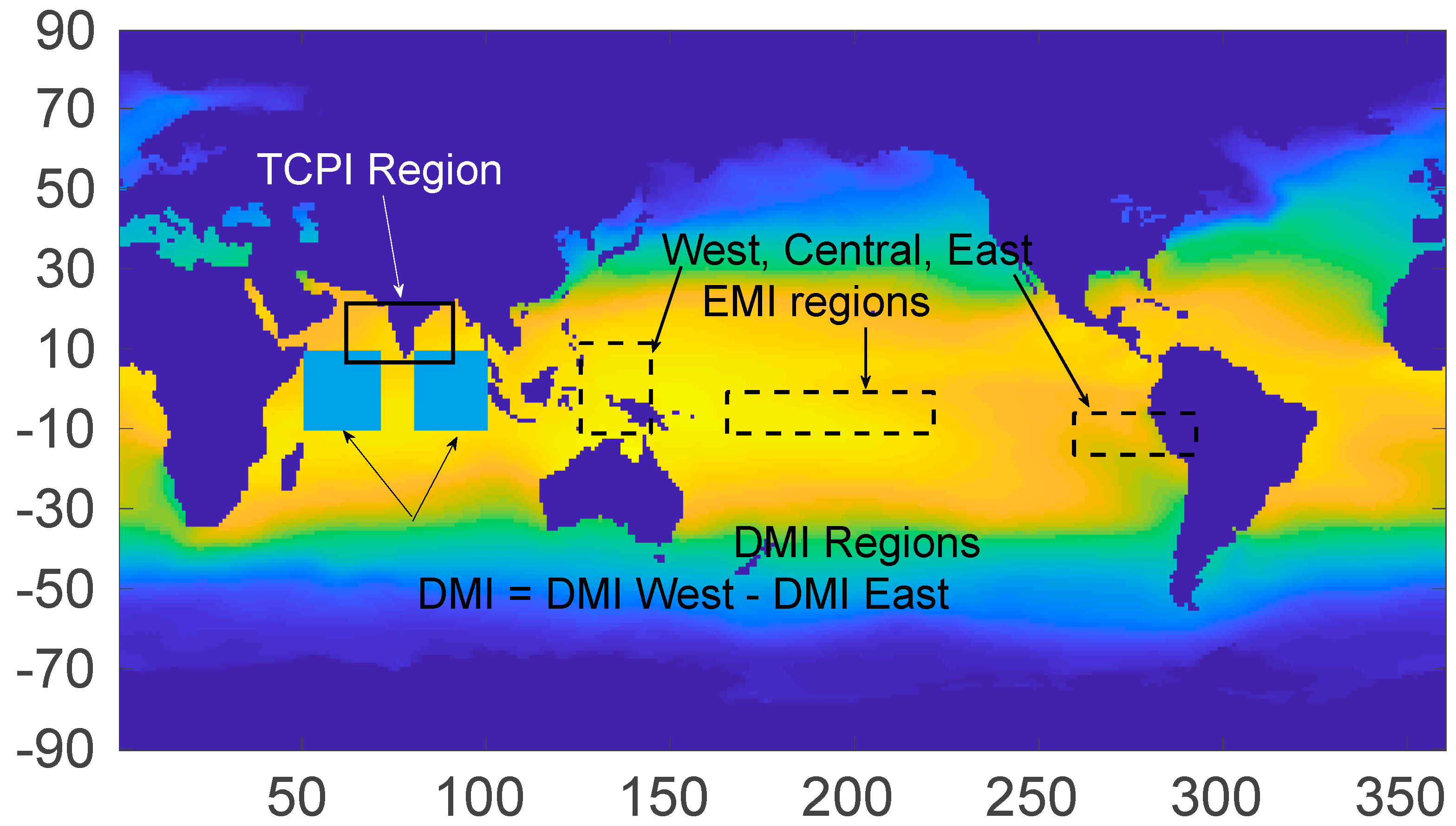
The difference in the SST between the western pole in the Arabian Sea and the eastern pole in the Bay of Bengal is termed as Dipole Mode Index (DMI). The DMI is a representative of the Indian Ocean Dipole (IOD) [20]. The western pole bounds the region 50° E-70° E and 10° S-10° N, and the eastern pole bounds the region 90° E-110° E and 10° S-0° [20].

Positive IOD is known to be positively connected to El Niño [21]. When the SST in the flanks surrounding central Pacific is cooler, El Niño Modoki is said to occur [14]. There is thus a possibility that when El Niño is negative, and so is IOD, the El Niño Modoki is likely to be positive.

This study aims to investigate the likely connection between the El Niño Modoki and the TCPI in the North Indian Ocean. Another purpose of the study is to investigate the missing link between these causal relationships. We also intend to discern how the DMI is connected to the El Niño Modoki in the Pacific and the TCPI in the Indian Ocean. The study primarily focuses on decadal patterns in the TC intensity.

The remaining part of the paper proceeds as follows:

• Section 2 discusses the datasets used (Section 2.1) and the methods (Section 2.2) employed in this study.
• Section 3 explains the observed results obtained from Empirical Mode Decomposition (EMD) (Section 3.1 and Section 3.2).
• Section 4 discusses the results with a possible explanation. This section also outlines the major conclusions of our investigation.

Recommendations for the future work are stated at the end of Section 4.

2. Data and Methods

2.1. Data

The data used in this study include:

• Gridded monthly SST, Atmospheric Temperature (AT) profile, Relative Humidity (RH) profile, Sea Level Pressure (SLP) reanalysis dataset at 1°X1° from National Oceanic and Atmospheric Administration (NCEP-NCAR-R1) [22].
• The results are verified using three independent datasets as follows:
  • Dataset 1: SST monthly dataset on a 2°X2° grid. The advantage of using this dataset is that it has improved spatial and temporal variability. This enhancement is done by (i) decreasing spatial filtering while training the reconstruction empirical orthogonal teleconnections, (ii) limiting high latitude damping in empirical orthogonal teleconnections, (iii) using unadjusted first guess instead of adjusted first guess [23,24]. (ftp://ftp.cdc.noaa.gov/Datasets/noaa.ersst.v5/sst.mnmean.nc)
  • Dataset 2: The globally extended monthly ocean temperature derived from a more extensive ICOADS release-2.5. This dataset offers better data due to bias adjustments, infiltrating procedures, and quality control. This is highly suitable for studies of climate variability and change. (https://climatedataguide.ucar.edu/climate-data/sst-data-noaa-extended-reconstruction-ssts-version-4)
  • Dataset 3: A global monthly SST analysis derived from the International Comprehensive Ocean-Atmosphere Data Set (ICOADS). The missing data is filled using statistical methods [25,26]. The data were interpolated in time and space by the providers. The data is taken from NOAA_ERSST_V3b data provided by the NOAA/OAR/ESRL PSD, Boulder, CO, USA, from their Web site at https://www.esrl.noaa.gov/psd/. The El Niño Modoki Index used here is defined as [14],

    $$EMI = \left[SSTA\right]Central – 0.5 \left[SSTA\right]East – 0.5\left[SSTA\right]West$$

    where, SSTA represents the area averaged SST over central (165°E−140°W, 10°S−10°N), Eastern (110°−70°W,15°S−5N), and Western (125°–145° E, 10°S−20°N). EMI refers to the El Niño Modoki Index. These regions are illustrated in Figure 1. (http://www.jamstec.go.jp/frsgc/research/d1/iod/modoki_home.html.en)
• Index (DMI). The DMI is computed using the three SST datasets defined above. The DMI is expressed as the difference between the SST gradient between the western equatorial Ocean (50°E–70°E and 10°S–10°N) and the southeastern equatorial Indian Ocean (90°E–110°E and 10°S–0°N) [20] (Figure 1).
• TCPI: Defined as per potential maximum wind speeds, it is computed using SST (all three datasets as above), atmospheric temperature, relative humidity, and sea level pressure datasets. The TCPI is evaluated using a method developed and explained by Bister and Emanuel [27].

2.2. Methods

The set of time series considered here could hold a multiple of periodic components. Thus a method that does not hold a priori hypothesis would prove to be most appropriate for analyses. EMD is such a power analysis tool without such consideration and is thus employed here.

The EMD method resulted in the constituent Intrinsic Mode Functions (IMFs). The physically significant IMFs (for instance, IMF 3) of each considered signal is used for further analysis.

Empirical Mode Decomposition (EMD)

Traditional time series methods like Fourier Transform, Wavelet transform offers an excellent approach to deal with climatic signals. However, these methods cannot efficiently deal with non-linear and non-stationary signals. Even though wavelet analysis is developed to deal with non-stationary signals, it fails to distinctly define local frequency changes. These traditional methods rely on a pre-assumed signal, mother wavelet in wavelet transform and sinusoidal signal in Fourier transform. EMD, on the other hand, does not make an assumption about linearity or stationarity. IMFs are generally simpler in interpretation and are relevant to physical phenomena being examined [28,29].

The method breaks down the considered signal within the time domain. The method decomposes the signal into its constituent IMFs by a method called shifting process. IMFs are defined by the following two main criteria,

• Single extreme zero crossings
• Zero mean values.

Consider a signal, X (t). On applying the cubic spline interpolation on the signal, an upper and a lower envelope of X (t) are generated. Let, m₁ be the mean of these envelopes. The first component say, $h_1$, is then given by the Equation (1),

$$h_{ 1}=X\left(t\right)- m_1$$

(1)

This is the first shifting process.

The second shifting process is repeated ‘k’ times (equation (2)) until $h_{1k}$ follows the IMF defining criterion where,

$$h_{ 1k}= h_{1\left(k-1\right)}- m_{1k}$$

(2)

The resultant h_1k is designated as, C₁. The component, C₁ denotes the first IMF of the signal (the Equation (3)) which is the shortest period component of the data. This is removed from the signal as,

$$X\left(t\right)- C_{1 }= r_1$$

(3)

Until we get a trend, this process continues. Selecting the physically meaningful modes:

EMD is a numerical method and is thus prone to numerical errors. These numerical errors may occur during the decomposition process. Therefore, the relevant and significant IMFs are sought before putting the modes for further usage. A highly suggested threshold method [30] is widely used before assigning statistical significance to the IMFs. The basis of the method lies in the fact that by definition, IMFs are supposed to be almost orthogonal components of the signal [30]. Thus, an acceptable IMF should have a relatively good correlation with the original signal. The IMFs with the correlation coefficient equal to or higher than the threshold value would be significant for further analysis. The threshold, λ, is defined as,

$$\lambda =\max \left(CCi\right)/N$$

(4)

where CC_i is the correlation coefficient of the ith mode and N represents the total number of IMFs. Max (CC_i) denotes the maximum correlation coefficient observed. The selection criterion for IMFs is as follows,

If CC_i>=λ, retain the ith IMF else, reject and eliminate it.

We employed Equation (4) on TCPI, DMI and EMI’s IMFs to retain the physically meaningful modes. The significant modes are kept and others are rejected. Only the retained modes are studied here but all the modes are shown and discussed.

TC Potential Intensity (TCPI) Computation:

TCPI is computed using a model developed by Emanuel [31]. The TC Potential Intensity (TCPI) represents the maximum sustained wind speeds at 10 m above the surface. TCPI is a better indicator of the threat of the storm than the frequency or intensity alone [32].

Considering a highly idealized axi-symmetric, steady-state TC, a model was developed [31] based on the following two primary assumptions. First, the flow above a well-mixed surface boundary layer is inviscid and secondly, it is thermodynamically reversible. These assumptions assured the safe usage of hydrostatic and gradient wind balance. Cd represents the surface drag coefficient which quantifies the resistance of an object in a fluid environment. According to Emanuel (1995)’s theory [33], a TC can maintain its kinetic energy if the energy supplied by oceanic heat sources is at a rate exceeding dissipation. Thus for a mature TC, Ce/Cd ranges as, 1.2 <Ce/Cd <1.5. At extreme winds, greater than 50 m/s, the drag coefficient found in most models causes kinetic energy to be destroyed. If Cd is set to 0, no system scale intensification occur [34]. The density of surface air fluctuates by 15% approximately and the drag coefficient Cd increases with cyclone’s wind speeds by a factor of 2. However, the Drag Coefficient settle around wind speeds of 30 ms⁻¹ [35].

The TCPI associated with TCs is quantitatively represented in the Equation (5),

$$TCPI=\sqrt[2]{\in \frac{C_k}{C_D}\left(k^{*}-k_B\right)}$$

(5)

where TCPI is represented at the radius of maximum winds.

3. Results

3.1. EMD Analysis

The first step of the study employs the EMD method. This mathematical tool breaks down a signal into its components called, IMFs. The resultant IMFs illustrates different causation parts of the composite signal. In the first sub-section, we discuss this intrinsic function for the TCPI in the North Indian Ocean. The second sub-section discusses the similar decomposition for El Niño Modoki, and the third sub-section the decomposition of DMI (or IOD).

3.1.1. EMD Analysis of TCPI

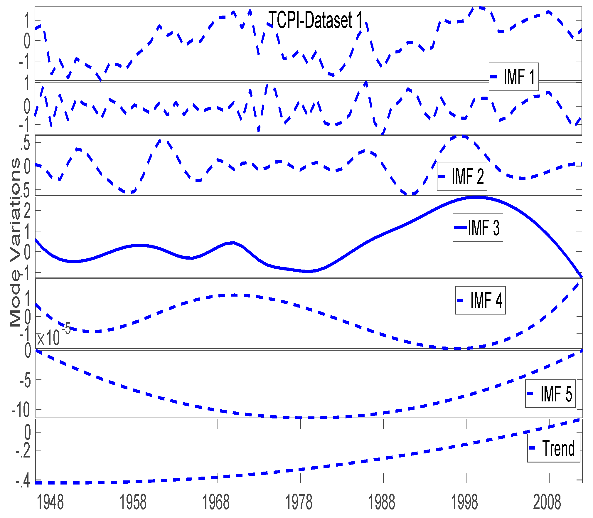
• EMD analysis of TCPI using Dataset-1

The EMD of TCPI in the North Indian Ocean as derived using Dataset-1 is shown in Figure 2. The top panel of the image represents the total composite signal. This signal is broken down into different causation parts called, IMFs. The third component (IMF 3) of the signal is used in the further analyses. We also notice monotonically increasing TCPI post-1958 (Figure 2, Panel 7)

Using Equation (4) on the correlation coefficients from

Table 1. Correlation Coefficient (CC) values of the TCPI modes and the signal derived from Dataset-1.

Signal-Mode Number	CC
Signal, IMF-1	0.4725
Signal, IMF-2	0.3382
Signal, IMF-3	0.4992
Signal, IMF-4	0.0753
Signal, IMF-5	0.0882
Signal, IMF-6 (Trend)	0.4853

, $\lambda$ = max (CC)/n, where, $\lambda$ = 0.50/6 = 0.08

Since the CC of all the modes (except IMF-4) is greater than $\lambda$, the modes shown in Figure 2 are significant of consideration. The highlighted mode, IMF-3 with highest CC is considered for further study.

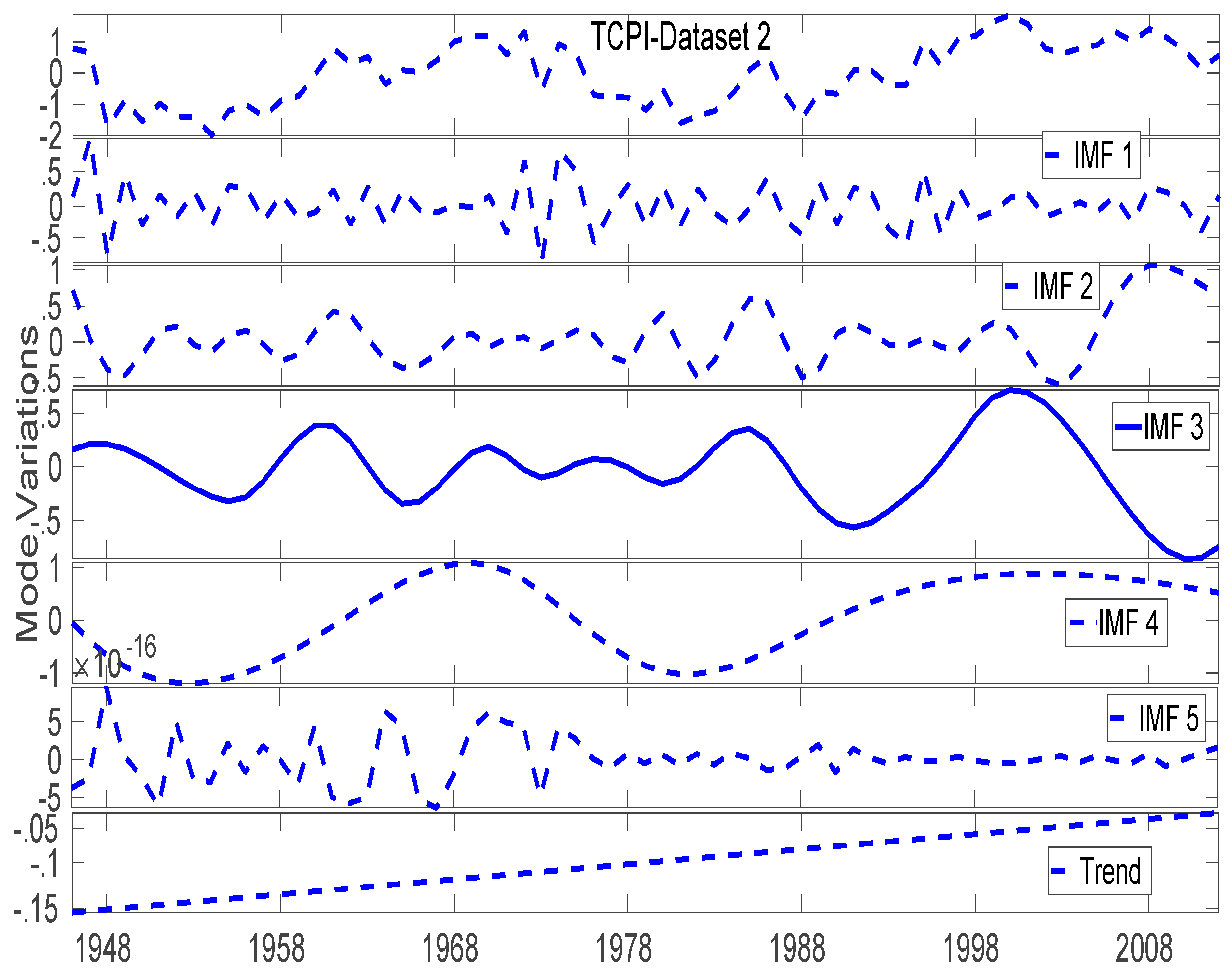
• EMD analysis of TCPI using Dataset-2:

Figure 3 illustrates the components of TCPI in the North Indian Ocean, derived using Dataset-2. The horizontal axis illustrates the time in years and the vertical axis represents the variation in the amplitude. The top panel of the image delineates the TCPI signal and its constituent modes are represented in the following panels. The significant intrinsic function, IMF3, is considered for further analysis.

The threshold value, $\lambda$= 0.50/6 = 0.08. Thus, we retained all the modes except the fifth one and consider the third mode (

Table 2. Correlation Coefficient (CC) values of the TCPI modes and the signal derived from Dataset-2.

Signal-Mode Number	CC
Signal, IMF-1	0.3582
Signal, IMF-2	0.4054
Signal, IMF-3	0.1858
Signal, IMF-4	0.8298
Signal, IMF-5	0.0692
Signal, IMF-6 (Trend)	0.5029

) for further analysis.

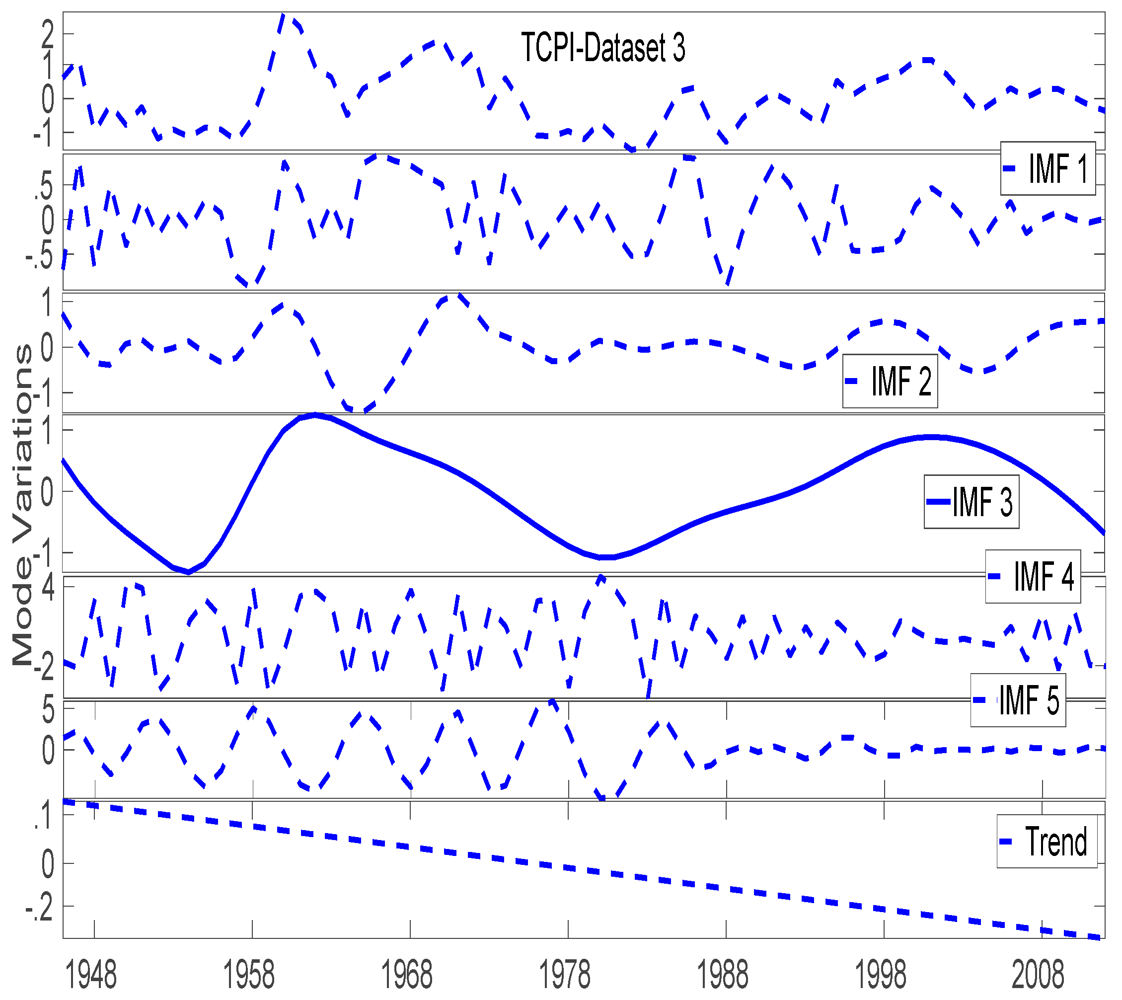
• EMD analysis of TCPI using Dataset-3:

Figure 4 illustrates the components of TCPI in the North Indian Ocean, derived using Dataset-3. The time in years is on the horizontal axis. The vertical axis represents the variation in the amplitude of the modes. The top panel of the image delineates the TCPI signal and its constituent modes are represented in the following panels. The significant intrinsic function, IMF3, is considered for further analysis in the later figures.

The threshold in this case is, $\lambda$ = 0.74/6 = 0.12. Thus, we can retain only the significant modes, IMF-1, 2, and 3.We further explore the mode (IMF-3,

Table 3. Correlation Coefficient (CC) values of the TCPI modes and the signal derived from Dataset-3.

Signal-Mode Number	CC
Signal, IMF-1	0.5319
Signal, IMF-2	0.3904
Signal, IMF-3	0.7451
Signal, IMF-4	0.0622
Signal, IMF-5	0.0698
Signal, IMF-6 (Trend)	0.0277

) with hthe ighest CC value in the next step.

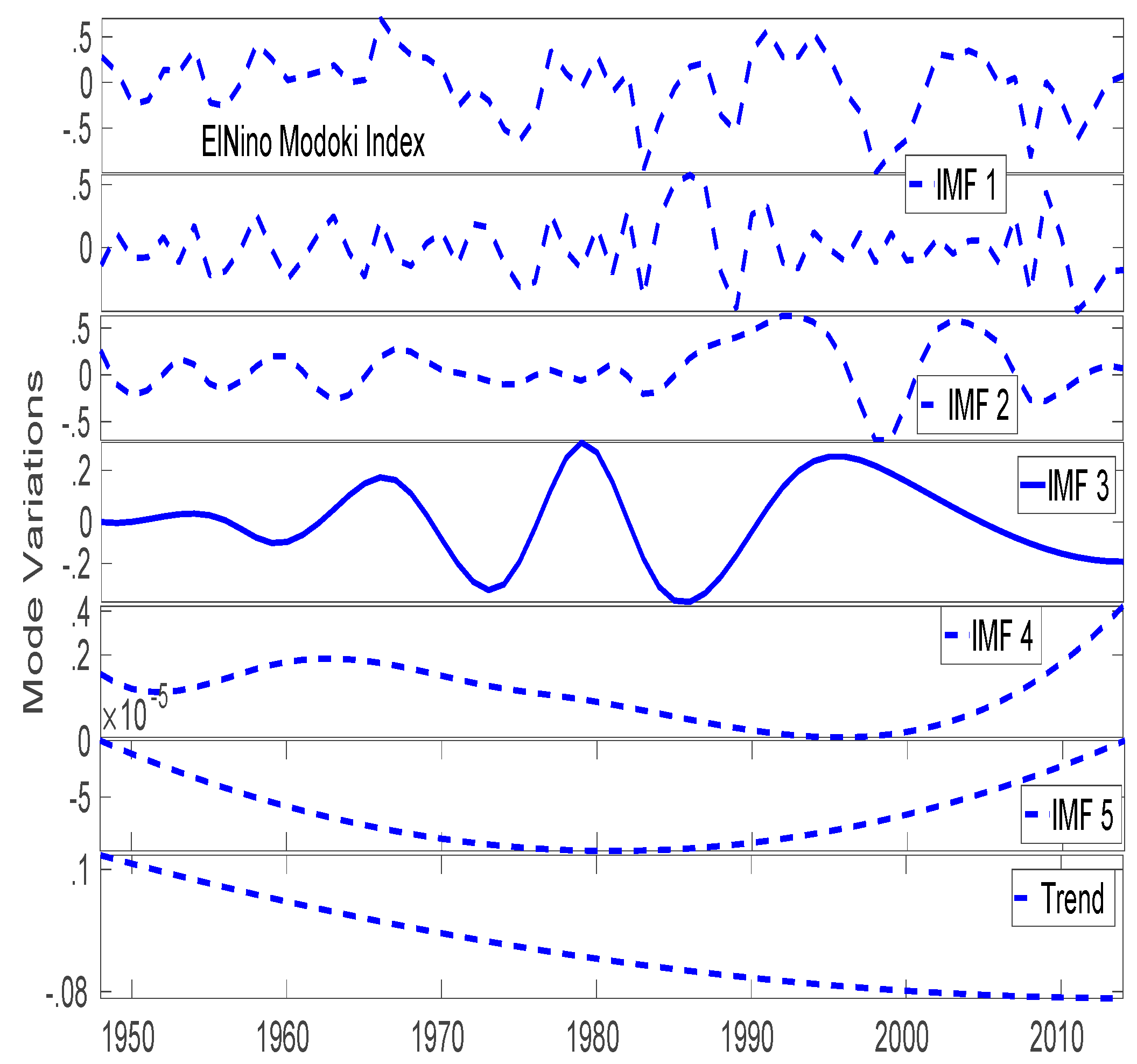
3.1.2. EMD Analysis of El Niño Modoki:

The causation modes of the El Niño Modoki are shown in Figure 5. El Niño Modoki signal is exhibited in the first panel of the figure and its trend in the last one. In between these, we see the composing modes of the primary El Niño Modoki signal. The signal shows a decreasing trend. The third mode, IMF3, is considered for further analysis.

The threshold in this case is, $\lambda$ = 0.66/6 = 0.11. Thus, we can retain only the significant modes, IMF-1, 2, 3 and 6. We further explore the mode (IMF-3,

Table 4. Correlation Coefficient (CC) values of the El Niño Modoki index and its modes.

Signal-Mode Number	CC
Signal, IMF-1	0.5010
Signal, IMF-2	0.6623
Signal, IMF-3	0.2448
Signal, IMF-4	0.0863
Signal, IMF-5	0.0074
Signal, IMF-6 (Trend)	0.2065

) in later figures.

3.1.3. EMD Analysis of DMI

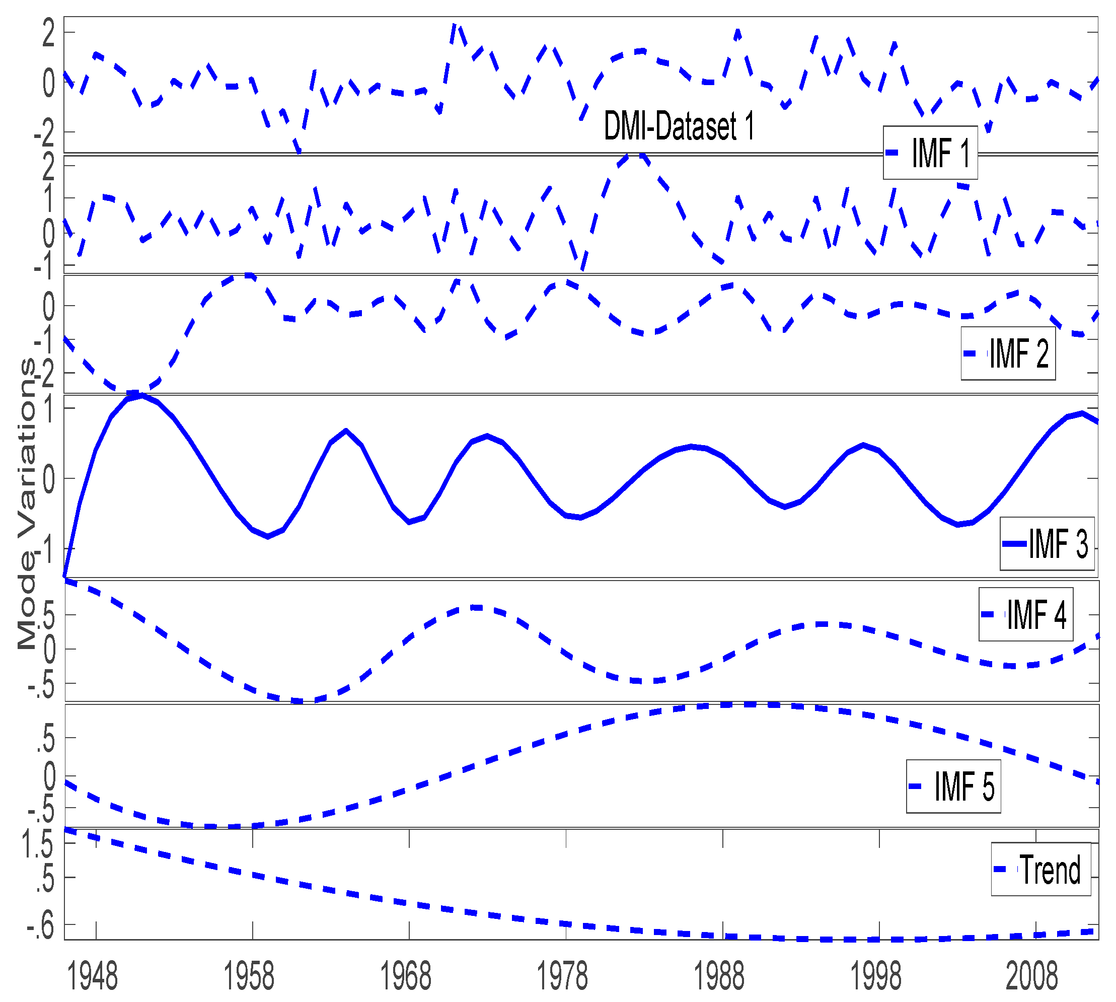
• EMD analysis of DMI using Dataset-1:

The variations in the DMI signal can be seen in the first panel of Figure 6. The trend of the DMI signal appears after the intrinsic modes of the signal. The significant third mode (panel 4) of the figure has been considered for further analysis as shown in a later figure.

Using the correlation coefficients from

Table 5. Correlation Coefficient (CC) values of the DMI modes and the signal derived from Dataset-1.

Signal-Mode Number	CC
Signal, IMF-1	0.6952
Signal, IMF-2	0.0932
Signal, IMF-3	0.1922
Signal, IMF-4	0.2649
Signal, IMF-5	0.2873
Signal, IMF-6 (Trend)	−0.1133

, the threshold, in this case, is $\lambda$ = 0.695/6 = 0.12. Thus, we can retain only the significant modes, IMF-1, 3, 4 and 5. We further explore the mode (IMF-3).

• EMD analysis of DMI using Dataset-2:

Figure 7 represents the primary DMI signal (Panel 1) and its corresponding intrinsic modes in panels 2 through 7. The DMI employed here is derived using sea surface temperature in the Dataset-2. The significant third mode of the signal has been employed for the analysis and is shown in a later figure.

Considering the correlation coefficients in

Table 6. Correlation Coefficient (CC) values of the DMI modes and the signal derived from Dataset-2.

Signal-Mode Number	CC
Signal, IMF-1	0.6921
Signal, IMF-2	0.2627
Signal, IMF-3	0.1661
Signal, IMF-4	0.2483
Signal, IMF-5	0.2759
Signal, IMF-6 (Trend)	0.0303

, the threshold, in this case, is $\lambda$ = 0.695/6 = 0.12. Thus, we can retain only the significant modes, IMF-1, 2, 3, 4 and 5. We further explore the mode (IMF-3).

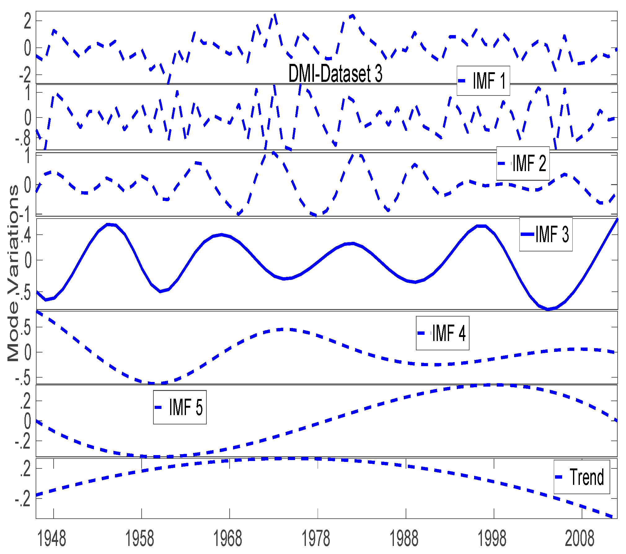
• EMD analysis of DMI using Dataset-3:

Figure 8 represents the primary DMI signal (Panel 1) and its corresponding intrinsic modes in panels 2 through 7. The DMI employed here is derived using sea surface temperature in the Dataset-3. The significant third mode of the signal has been employed for the analysis as shown in a figure later on.

The DMI signal is shown in the first panel and its trend in the seventh panel. The intrinsic modes of the signal are presented in between these two panels. The retained mode considered for further analysis is shown with a bold line.

The threshold in this case is, $\lambda$ = 0.72/6 = 0.13 (

Table 7. Correlation Coefficient (CC) values of the DMI modes and the signal derived from Dataset-3.

Signal-Mode Number	CC
Signal, IMF-1	0.7190
Signal, IMF-2	0.4684
Signal, IMF-3	0.2175
Signal, IMF-4	0.2271
Signal, IMF-5	0.1278
Signal, IMF-6 (Trend)	0.2225

). Thus, we can retain only the significant modes, IMF-1, 2,3, 4 and 6 and we further explore the mode (IMF-3).3.2.

3.2. Mode Comparison

Changes in the TCPI, DMI and El Niño Modoki signal have been compared here using the third modes of the signals.

We hypothesized that there are more chances of having a low TC activity during the El Niño Modoki period than during the normal season. The IOD acts as a mechanism to explain this observation.

During the El Niño Modoki period, the Walker circulation breaks into two sub circulations. A part of which descends over the east of the North Indian Ocean, near the Philippines. This hinders the disturbance formation in the Bay of Bengal and subsequently the tropical cyclone activity over the region. An anomalously colder region over the West of central Pacific (towards North Indian Ocean) could propagate into the Bay of Bengal. Negative IOD indicates lower sea surface temperature over the Bay of Bengal than over the Arabian Sea. Less than normal disturbance propagation and lower sea surface temperature, both of which are the primary ingredients of tropical cyclone genesis, means a dip in the TCPI. Thus, a peak in the El Niño Modoki mode (EMI) would manifest as a dip in the IOD and also the TCPI.

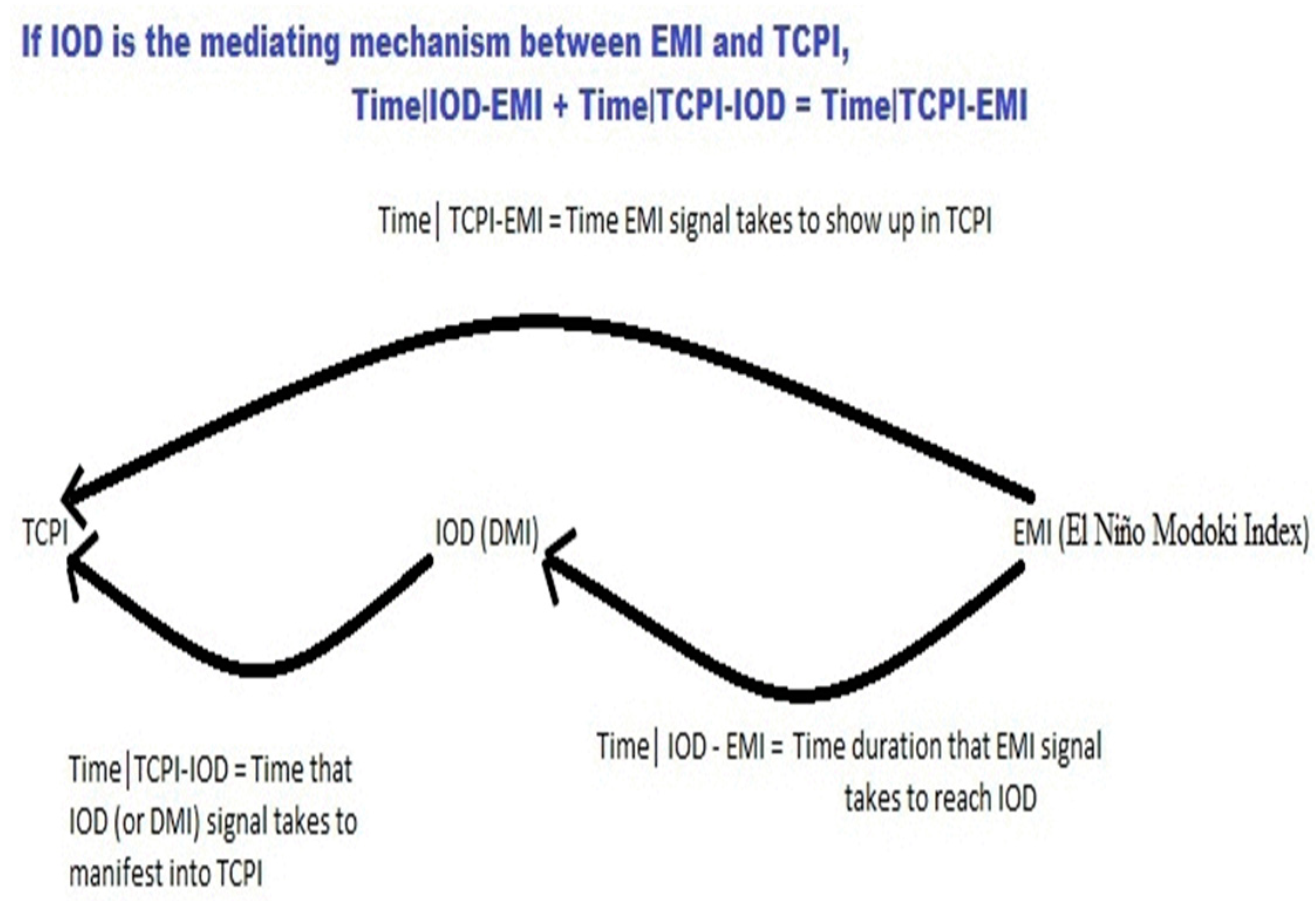
IOD as a mediating mechanism between TCPI and EMI:

Secondly, if IOD acts as a mediating mechanism between the TCPI and EMI, the total time EMI takes to propagate its effect on TCPI (Figure 9) should be equal to the sum of the time interval between IOD & EMI, and that between TCPI and IOD.

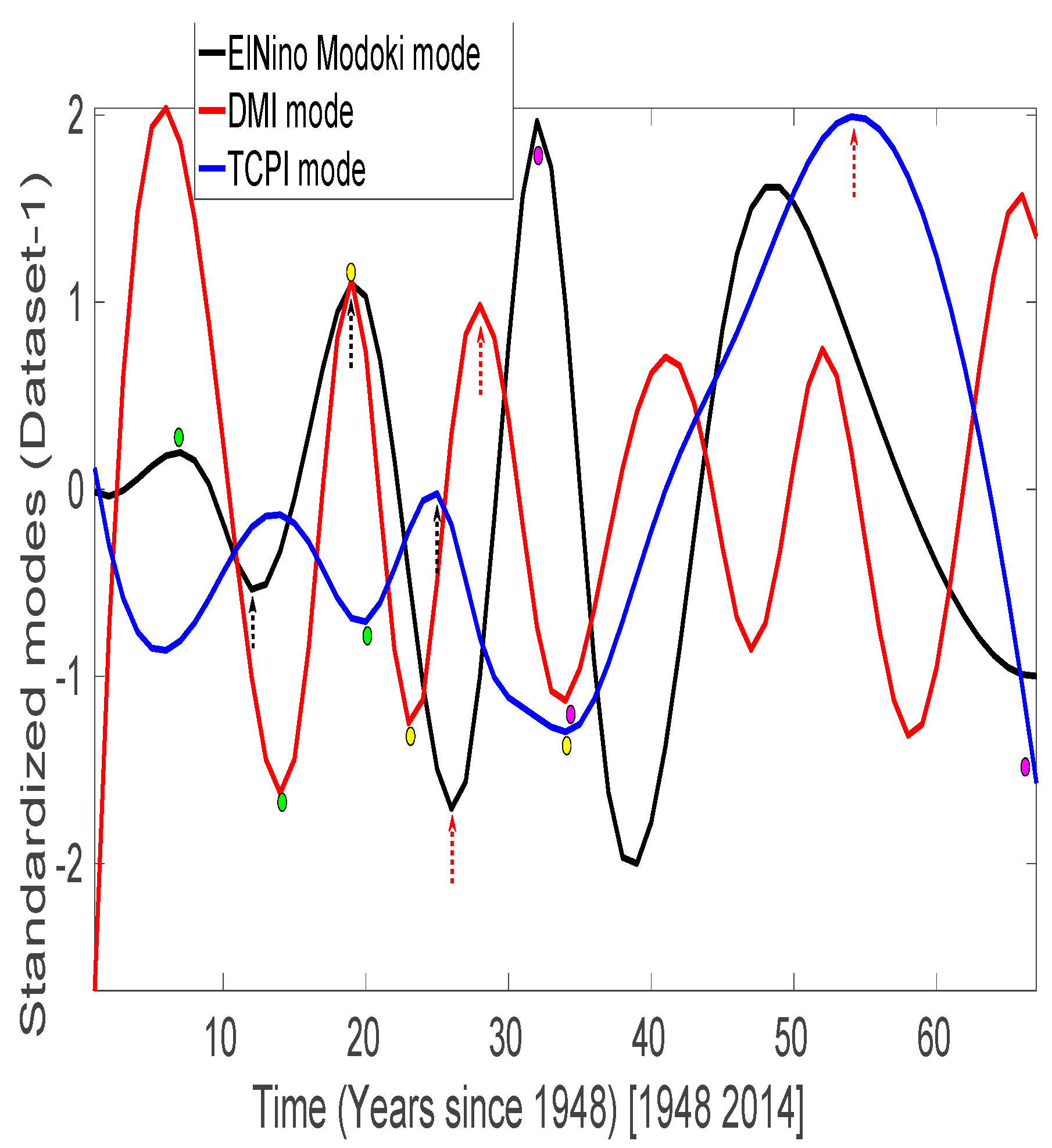
3.2.1. Mode Comparison between TCPI, DMI and El Niño Modoki: Dataset-1

The third modes of the TCPI, DMI and El Niño Modoki signals (EMI) derived using Dataset-1 are used here for a comparative study. It is apparent from Figure 10, Figure 11 and Figure 12 that the peak (trough) in the El Niño Modoki leads the dip (crest) in the DMI signal in the North Indian Ocean which is, in turn, leads the dip (trough) in the TCPI signal in the North Indian Ocean.

The X-axis in the Figure 10, Figure 11 and Figure 12 represents time, in years, since 1948 and Y-axis shows the variations in the third modes (IMF 3) of all the three variables, TCPI, DMI, and EMI.

What can be clearly seen in

Table 8. Peaks in the EMI (Figure 10) and the corresponding valleys in the DMI followed by a dip in the TCPI.

EMI Maxima	7	19	32
DMI minima	14	23	34
TCPI minima	20	34	67+
Interval DMI-EMI:	7	4	2
Interval TCPI-DMI:	6	11	NA
Interval TCPI-EMI:	13	15	NA

(and corresponding Figure 10) is that a peak in the El Niño Modoki mode (7, 19) leads the dip in DMI signal (14, 23). This dip in the DMI then leads the TCPI minima (20, 34). Thus, the corresponding yearly time interval between the EMI and DMI being 7 and4 respectively while that between TCPI and DMI is 6 and 11. If IOD is the link between EMI and TCPI, the total time between EMI and TCPI thus should be 13 (7+6) and 15 (4+11). The last row of Table 8 indicates the total time duration between EMI and TCPI of 13 and 15 years respectively and corroborates with our hypothesis.

Similarly,

Table 9. Minima in the EMI (Figure 10) and the corresponding local maxima in the DMI followed by a dip in the TCPI.

EMI minima	12	26
DMI maxima	19	28
TCPI maxima	25	54
Interval DMI-EMI:	7	2
Interval TCPI-DMI:	6	26
Interval TCPI-EMI:	13	28

shows that a dip in the EMI (12, 26) and the corresponding peaks in the DMI (19, 28) are followed by peaks in TCPI (25, 54). The time interval between EMI and DMI (7,2) and that between DMI and TCPI (6,26) sum up to the total time between EMI and TCPI (7+6,2+26). This is the same as the time intervals between EMI dips and the corresponding TCPI peaks (13, 28), last row of Table 9 which again justifies our hypothesis.

Associated peaks and valleys in the modes are shown with similar markings, coloured dots or arrows.

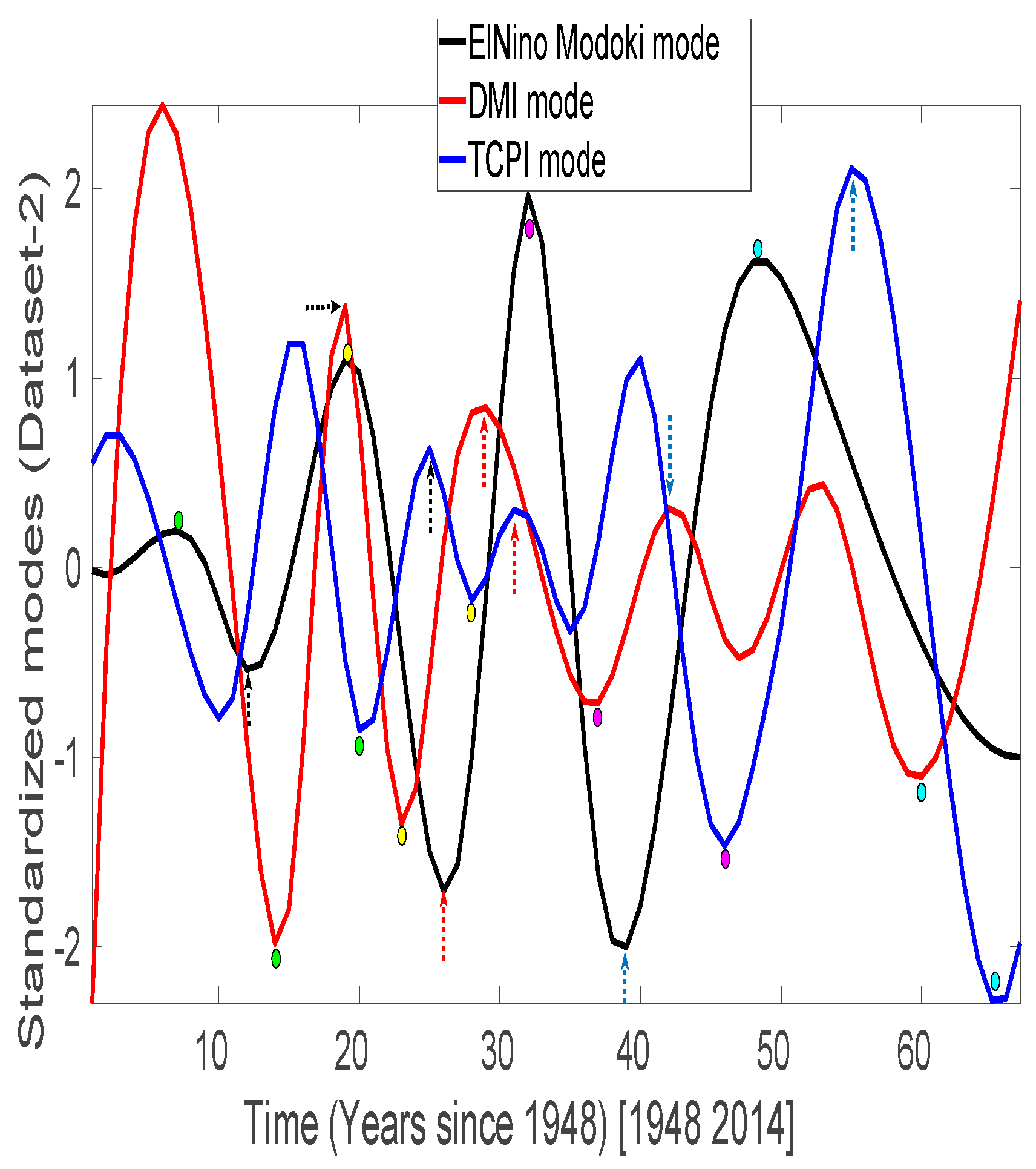
3.2.2. Mode Comparison between TCPI, DMI and El Niño Modoki: Dataset-2

Figure 11 presents a comparison between the TCPI, DMI and El Niño Modoki modes. The TCPI and DMI modes used here are derived using Dataset-2. As in the previously discussed figure, we notice El Niño Modoki as one of the contributors to the TCPI fluctuations in the North Indian Ocean. DMI, shown in red, links the two modes.

What stands out in

Table 10. Peaks in the EMI (Figure 11) and the corresponding valleys in the DMI followed by a dip in the TCPI.

EMI maxima	7	19	32	48
DMI minima	14	23	37	60
TCPI minima	20	28	46	65
Interval DMI-EMI:	7	4	5	12
Interval TCPI-DMI:	6	5	9	5
Interval TCPI-EMI:	13	9	14	17

(and the related Figure 11) is that a peak in the El Niño Modoki mode (7, 19, 32, and 48) leads the dip in DMI signal (14, 23, 37, and 60). This dip in the DMI then leads the TCPI minima (20, 28, 46 and 65). Thus, the corresponding time interval between the EMI and DMI being 7, 4, 5 and 12 while that between TCPI and DMI is 6, 5, 9 and 5. If IOD is the link between EMI and TCPI, the total time between EMI and TCPI thus should be 13 (7+6), 9 (4+5), 14(5+9) and 17(12+5). The last row of Table 10 indicates the total time duration between EMI and TCPI which is 13, 9, 14 and 17.

Table 11. Minima in the EMI (Figure 11) and the corresponding local maxima in the DMI followed by a dip in the TCPI.

EMI minima	12	26	39
DMI maxima	19	29	42
TCPI maxima	25	31	55
Interval DMI-EMI:	7	3	3
Interval TCPI-DMI:	6	2	13
Interval TCPI-EMI:	13	5	16

shows that a dip in the EMI (12, 26, and 39) and the corresponding peaks in the DMI (19, 29, and 42) are followed by peaks in TCPI (25, 31, and 55). The time interval between EMI and DMI (7, 3, 3) and that between DMI and TCPI (6, 2, 13) sum up to the total time between EMI and TCPI (7+6, 3+2, 3+13). This is the same as the time intervals between EMI dips and the corresponding TCPI peaks (13, 5, and 16), the last row of Table 11.

However, it should be noted that a dip in the El Niño Modoki in 1968 leads the peaks in DMI and again, El Niño Modoki seems to oppose the TCPI and IOD signals.

Corresponding peaks and troughs in the modes are shown with similar markings, coloured dots or arrows.

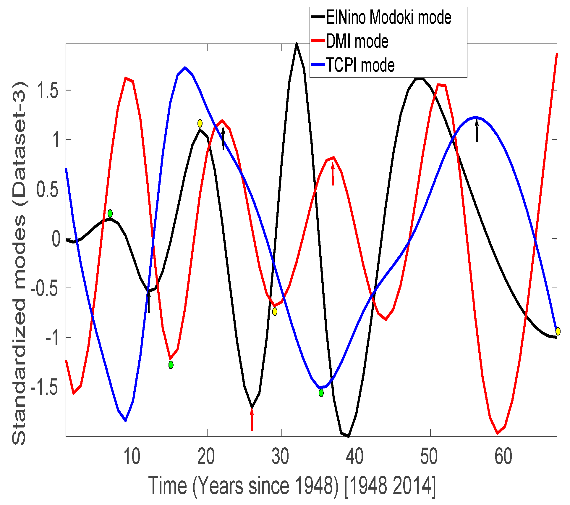
3.2.3. Mode Comparison between TCPI, DMI and El Niño Modoki: Dataset-3

A connection between the TCPI, DMI and El Niño Modoki modes are shown in Figure 12. TCPI and DMI modes are derived using Dataset-3. Again, we see DMI as a mediating agent between the El Niño Modoki and TCPI phenomena, similar to as seen in Figure 10 and Figure 11).

What is interesting in

Table 12. Peaks in the EMI (Figure 12) and the corresponding valleys in the DMI followed by a dip in the TCPI.

EMI maxima	7	19
DMI minima	13	29
TCPI minima	35	67+
Interval DMI-EMI:	6	10
Interval TCPI-DMI:	22	NA
Interval TCPI-EMI:	28	NA

(and the related Figure 12) is that a peak in the El Niño Modoki mode (7) leads the dip in DMI signal (13). This dip in the DMI then leads the TCPI minima (35). Thus, the corresponding time interval between the EMI and DMI being 6 while that between TCPI and DMI is 22. If IOD is the link between EMI and TCPI, the total time between EMI and TCPI thus should be 28 (6+22). The last row of Table 12 indicates the total time duration between EMI and TCPI which is, 28, supporting our assumption.

Table 13. Minima in the EMI (Figure 12) and the corresponding local maxima in the DMI followed by a dip in the TCPI.

EMI minima	12
DMI maxima	22
TCPI maxima	56
Interval DMI-EMI:	10
Interval TCPI-DMI:	34
Interval TCPI-EMI:	44

shows that a dip in the EMI (12) and the corresponding peaks in the DMI (22) is followed by peaks in TCPI (56). The time interval between EMI and DMI (10) and that between DMI and TCPI (34) sum up to the total time between EMI and TCPI (10+34). This is the same as the time interval between EMI dips and the corresponding TCPI peaks (44), the last row of Table 13.

Associated crests and troughs in the modes are shown with similar markings, coloured dots or arrows.

From Figure 10, Figure 11 and Figure 12, and values in Table 8, Table 9, Table 10, Table 11, Table 12 and Table 13, it could conceivably be hypothesized that IOD acts as a commuting mechanism between El Niño Modoki and TCPI in the North Indian Ocean.

The most interesting aspect to emerge from this section is the relation between the El Niño Modoki, DMI and TCPI. DMI here demonstrates as an energy exchange mechanism between the El Niño Modoki and the TCPI. Based on this, we may infer that one of the new phenomena of interest to the climate community, El Niño Modoki, influence the regional TCPI in the North Indian Ocean with IOD acting as a connecting mechanism.

A possible explanation of this connection could be that the El Niño period is characterized by an anomalously cooler temperature in the western Pacific, towards the Indian Ocean (Bay of Bengal). The Arabian Sea during this season sees comparatively more or stronger TCs due to the available disturbance from the ascending circulation in the west of Arabian Sea. This is the time when the Arabian Sea sees a higher temperature than the Bay of Bengal and IOD is usually positive. However, Bay of Bengalis relatively warmer than the Arabian Sea during El Niño Modoki season and produce a comparable or higher number or intensity of TCs. This is because, during the El Niño Modoki period, the SST towards the West Pacific is comparatively warmer than during the El Niño period. The comparatively higher temperature in the Bay of Bengal indicates a negative IOD. The Walker circulation descending over the Philippines and Indonesia limit the disturbance propagation towards the Bay of Bengal.

A negative IOD, associated with, lowering of the TCs over the Arabian Sea and less than adequate temperature over the Bay of Bengal combined with the lack of disturbance propagation subsequently lowers the annual depression formation and the TCPI in the NIO.

For IOD to act as an intermediate mechanism between the TCPI and EMI, the total time that EMI takes to propagate its effect on TCPI (Figure 9) should be equal to the sum of the time intervals between IOD & EMI, and that between TCPI & IOD.

4. Discussion and Conclusions

El Niño Modoki and TCPI relation explained with IOD (or DMI) as a missing link.

Result presented here is in line with a familiar work on TC formation in the Indian Ocean during El Niño Modoki events [21]. The research work explained the impact of El Niño Modoki events on TC genesis in the Indian Ocean using IOD data in the same location. Our work extends this knowledge with rigorous analysis of the impact of El Niño Modoki on the TCPI in the Indian Ocean. The causal link to this connection was found to be via the dipole index (IOD or DMI).

Since the datasets considered here are highly non-stationary in nature, we are not associating periodicities using simple methods. More sophisticated methods like wavelets would be required here to handle such signals.

Also, El Niño Modoki does not strictly follow a periodic occurrence resulting in irregular oscillatory associations with IOD and TCPI. Thus, we cannot associate the exact time intervals of the mediation here but what can be inferred from the results is that IOD presents itself as a commuting mechanism between the El Niño Modoki and TCPI.

5. Future Work

A natural progression of this work is to analyze and find the cause of the observed relationship between the El Niño Modoki, IOD and TCPI.

Despite these promising results, an accurate energetic based mechanism to quantitatively explain the cause and effect relationship between the TCPI and El Niño Modoki via IOD is indispensable.

Further research could usefully explore this relation using a longer dataset.

References

- Landsea, C.W.; Nicholls, N.; Gray, W.M.; Avila, L.A. Downward trends in the frequency of intense Atlantic hurricanes during the past five decades. Geophys. Res. Lett. 1996, 3, 1697–1700. [Google Scholar] [CrossRef]
- Chan, J.C.L.; Shi, J.-E. Long-term trends and interannual variability in tropical cyclone activity over the western North Pacific. Geophys. Res. Lett. 1996, 23, 2765–2767. [Google Scholar] [CrossRef]
- Emanuel, K. Increasing destructiveness of tropical cyclones over the past 30 years. Nature 2005, 436. [Google Scholar] [CrossRef] [PubMed]
- Bhatia, K. Projected response of tropical cyclone intensity and intensification in global climate model. AMS J. Clim. 2018. [Google Scholar] [CrossRef]
- Knutson, T.R.; McBride, J.L.; Chan, J.; Emanuel, K.; Holland, G.; Landsea, C.; Held, I.; Kossin, P.; Srivastava, K.; Sugi, M. Tropical cyclones and climate change. Nat. Geosci. 2010, 3, 157–163. [Google Scholar] [CrossRef] [Green Version]
- Lewis, S.C.; LeGrande, A.N. Stability of ENSO and its tropical Pacific teleconnections over the last millennium. Clim. Past 2015, 11, 1347–1360. [Google Scholar] [CrossRef]
- Arora, K.; Dash, P. Towards dependence of tropical cyclone intensity on sea surface temperature and its response in a warming world. Climate 2016, 4, 30. [Google Scholar] [CrossRef]
- Chan, J.C.L. Tropical cyclone activity in the northwest Pacific in relation to the El Nino/Southern Oscillation phenomenon. Mon. Weather Rev. 1985, 113, 599–606. [Google Scholar] [CrossRef]
- Wang, B.; Chan, J.C.L. How strong ENSO events affect tropical storm activity over the western North Pacific. J. Clim. 2002, 15, 1643–1658. [Google Scholar] [CrossRef]
- Chu, P.-S.; Murnane, R.J.; Liu, K.B. (Eds.) ENSO and Tropical Cyclone Activity. In Hurricanes and Typhoons: Past, Present, and Future; Columbia University Press: New York, NY, USA, 2004; pp. 297–332. [Google Scholar]
- Camargo, S.J.; Emanuel, K.A.; Sobel, A.H. Use of a genesis potential index to diagnose ENSO effects on tropical cyclone genesis. J. Clim. 2007, 20, 4819–4843. [Google Scholar] [CrossRef]
- Landsea, C.W.; Pielke, R.A., Jr.; Mestas-Nuñez, A.M.; Knaff, J.A. Atlantic basin hurricanes: Indices of climatic changes. Clim. Chang. 1999, 42, 89–129. [Google Scholar] [CrossRef]
- Elsner, J.B.; Kara, A.B. Hurricanes of the North Atlantic: Climate and Society; Oxford University Press: New York, NY, USA, 1999; 488p. [Google Scholar]
- Ashok, K.; Behera, S.K.; Rao, S.A.; Weng, H. El-Niño Modoki and its possible teleconnections. J. Geophys. Res. 2007, 112, C11007. [Google Scholar] [CrossRef]
- Weng, H.; Ashok, K.; Behera, S.K.; Rao, S.A.; Yamagata, T. Impacts of recent El Niño Modoki on dry/wet conditions in the Pacific rim during boreal summer. Clim. Dyn. 2007, 29, 113–129. [Google Scholar] [CrossRef] [Green Version]
- Cayan, D.R.; Dettinger, M.D.; Diaz, H.F.; Graham, N.E. Decadal variability Decadal variability of precipitation over western North America. J. Clim. 1998, 11, 3148–3166. [Google Scholar] [CrossRef]
- Barlow, M.; Nigam, S.; Berbery, E.H. ENSO, Pacific decadal variability, and U. S. summertime precipitation, drought, and stream flow. J. Clim. 2001, 14, 2105–2128. [Google Scholar] [CrossRef]
- Hu, Q.; Feng, S. Variations of teleconnection of ENSO and interannual variation in summer rainfall in the central United States. J. Clim. 2001, 14, 2469–2480. [Google Scholar] [CrossRef]
- Seager, R.; Kushnir, Y.; Herweijer, C.; Niak, N.; Velez, J. Modeling of tropical forcing of persistent droughts and pluvials over western North America: 1856–2000. J. Clim. 2005, 18, 4065–4088. [Google Scholar] [CrossRef]
- Saji, N.H.; Goswami, B.N.; Vinayachandran, P.N.; Yamagata, T. A dipole mode in the tropical Indian Ocean. Nature 1999, 401, 360–363. [Google Scholar] [CrossRef] [PubMed]
- Sumesh, K.G.; Kumar, M.R.R. Tropical cyclones over north Indian Ocean during El-Niño Modoki years. Nat. Hazards 2013, 68, 1057–1074. [Google Scholar] [CrossRef]
- Kalnay, E.; Kanamitsu, M.; Kistler, R.; Collins, W.; Deaven, D.; Gandin, L.; Iredell, M.; Saha, S.; White, G.; Woollen, J.; et al. The NCEP/NCAR 40 year reanalysis project. Bull. Am. Meteorol. Soc. 1996. [Google Scholar] [CrossRef]
- Huang, B.; Banzon, V.F.; Freeman, E.; Lawrimore, J.; Liu, W.; Peterson, T.C.; Smith, T.M.; Thorne, P.W.; Woodruff, S.D.; Zhang, H.-M. Extended Reconstructed Sea Surface Temperature version 4 (ERSST.v4): Part I. Upgrades and intercomparisons. J. Clim. 2014, 28, 911–930. [Google Scholar] [CrossRef]
- Liu, W.; Huang, B.; Thorne, P.W. Extended Reconstructed Sea Surface Temperature version 4 (ERSST.v4): Part II. Parametric and structural uncertainty estimations. J. Clim. 2014, 28, 931–951. [Google Scholar] [CrossRef]
- Smith, T.M.; Reynolds, R.W.; Peterson, T.C.; Lawrimore, J. Improvements NOAAs Historical Merged Land–Ocean Temp Analysis (1880–2006). J. Clim. 2008, 21, 2283–2296. [Google Scholar] [CrossRef]
- Xue, Y.; Smith, T.M.; Reynolds, R.W. Interdecadal Changes of 30-Yr SST Normals during 1871–2000. J. Clim. 2003, 16, 1601–1612. [Google Scholar] [CrossRef]
- Bister, M.; Emanuel, K.A. Dissipative heating and hurricane intensity. Meteorol. Atmos. Phys. 1998, 55, 233–240. [Google Scholar] [CrossRef]
- Huang, N.E.; Shen, Z.; Long, S.R.; Wu, M.C.; Shih, H.H.; Zheng, Q.; Yen, N.-C.; Tung, C.C.; Liu, H.H. The empirical mode decomposition and the Hilbert spectrum for nonlinear and non-stationary time series analysis. Proc. R. Soc. Lond. 1998, 454, 903–993. [Google Scholar] [CrossRef]
- Huang, N.E.; Shen, Z.; Long, S.R. A new view of nonlinear water waves-The Hilbert spectrum. Annu. Rev. Fluid Mech. 1999, 31, 417–457. [Google Scholar] [CrossRef]
- Peng, Z.K.; Tse Peter, W.; Chu, F.L. A comparison study of improved Hilbert Huang transform and wavelet transform: Application to fault diagnostics for rolling bearing. Mech. Syst. 2005, 19, 974–988. [Google Scholar] [CrossRef]
- Emanuel, K.A. An air-sea interaction theory for tropical cyclones, Part 1. J. Atmos. Sci. 1986, 42, 1062–1071. [Google Scholar] [CrossRef]
- Emanuel, K.; Ravela, S.; Vivant, E.; Risi, C. A combined statistical-deterministic approach of hurricane risk assessment. Unpublished manuscript. 2005. [Google Scholar]
- Emanuel, K.A. The behavior of a simple hurricane model using a convective scheme based on sub-cloud layer entropy equilibrium. J. Atmos. 1995, 52, 3960–3968. [Google Scholar] [CrossRef]
- Montgomery, M.T.; Smith, R.K.; Nguyen, S.V. Sensitivity of tropical-cyclone modelsto the surface drag coefficient. RMetS 2010, 136, 1945–1953. [Google Scholar]
- Powell, M.D.; Vickery, P.J.; Reinhold, T.A. Reduced drag coefficient for high wind speeds in tropical cyclones. Nature 2003, 422, 279–283. [Google Scholar] [CrossRef] [PubMed]
Figure 1.
The spatial domains where TCPI, DMI and El Niño Modoki datasets are considered. TCPI is in the North Indian Ocean, DMI regions are south of the TCPI region. The image has SST values over the sea surface and the land is masked in the algorithm. DMI is computed as the difference between the western and the eastern regions, as shown. The El Niño Modoki regions are illustrated with dashed lines.
Figure 2.
EMD analysis of the TCPI signal in the North Indian Ocean. TCPI derived using Dataset-1. The signal is shown in the first panel. The following panels illustrate its intrinsic modes. The trend of the signal shows a rise from 1958 onwards (Panel-7).
Figure 3.
The EMD analysis of the TCPI signal in the North Indian Ocean. TCPI used here is derived using Dataset-2. The derived signal is shown in the first panel and its increasing trend in the seventh panel.
Figure 4.
The EMD analysis of the TCPI signal in the North Indian Ocean. TCPI used here is derived using Dataset-3. The derived signal is shown in the first panel and its trend in the seventh panel. The third mode (IMF 3) retained for further analysis is shown in bold.
Figure 5.
EMD analysis of the El Niño Modoki index. The El Niño Modoki index is shown in the first panel and its trend in the seventh panel. The causation modes of the signals are presented in between these two panels. The retained mode is shown with a bold line (IMF 3).
Figure 6.
An EMD analysis of the DMI signal in the North Indian Ocean. The signal here is derived using the Dataset-1. The DMI signal is shown in the first panel and its monotonically increasing trend in the seventh panel. The causation modes of the signals are presented in between these two panels.
Figure 7.
The EMD of the DMI signal in the North Indian Ocean is illustrated in the adjoining figure. The signal here is derived using the Dataset-2. The DMI signal is shown in the first panel and its trend in the seventh panel. The intrinsic modes of the signal are presented in between these two panels. The retained mode considered for further analysis is shown in a bold line (IMF 3).
Figure 8.
The EMD of the DMI signal in the North Indian Ocean is illustrated in the adjoining figure. The signal here is derived using the Dataset-3.
Figure 9.
IOD as a mediating mechanism between the El Niño Modoki and tropical cyclones over the North Indian Ocean.