Retrospective Analysis of Summer Temperature Anomalies with the Use of Precipitation and Evapotranspiration Rates

Abstract

Drought and extreme temperatures forecasting is important for water management and the prevention of health risks, especially in a period of observed climatic change. A large precipitation deficit together with increased evapotranspiration rates in the preceding days contribute to exceptionally high temperature anomalies in the summer above the average local maximum temperature for each month. Using a retrospective approach, this study investigated droughts and extreme temperatures in the greater area of Nicosia, Cyprus and suggests a different approach in determining the lag period of summer temperature anomalies and precipitation. In addition, dry conditions defined with the use of the Standardized Precipitation-Evapotranspiration Index (SPEI) were associated with positive temperature anomalies at a percentage up to 33.7%. The compound effect of precipitation levels and evapotranspiration rates of the preceding days for the period 1988–2017 to summer temperature anomalies was demonstrated with significantly statistical R squared values up to 0.57. Furthermore, the cooling effect of precipitation was higher and prolonged longer in rural and suburban than urban areas, a fact that is directly related to the evaporation potential of the area in concern. Our work demonstrates the compound effect of precipitation levels and evapotranspiration rates of the preceding days to summer temperature anomalies.

1. Introduction

Weather regimes drive climate change and influence temperature variation [1] and may persist from a few days to a few weeks. Weather regimes in Cyprus depend on mid-latitude flow dynamics, yet they are regulated by several external factors, such as dry soils [2,3] and sea-surface temperature anomalies [4,5] that subsequently affect the development and the duration of heat waves. The feasibility of prediction of extreme temperatures in the summer using numerical models largely rests on the variability of soil moisture, sea surface temperature, and heat fluxes [6]. Variations of surface temperature after a precipitation event in the summer suggest that, due to the wet ground, more energy is likely to go into evaporation at the expense of sensible heating [7,8]. Precipitation is also associated with clouds blocking the sun and provides less energy by further reducing the temperature [7,9].

Hirschi et al. [10] divided the European domain into two sectors based on the soil moisture variations: southeast Europe with transitional soil-moisture-limited evapotranspiration regime and central European characterized by a wet soil-moisture regime (energy-limited evapotranspiration regime) [10]. A strong relationship between soil-moisture deficit and summer hot extremes in southeast Europe was noted. Droughts and heatwaves have been shown to intensify and propagate via land–atmosphere feedbacks [3]. Fischer et al. [2] argued that a large precipitation deficit together with early vegetation green-up and strong positive radiative anomalies in the months preceding the extreme summer event contributed to an early and rapid loss of soil moisture [2], resulting in low latent cooling and increased temperatures. Soil moisture deficits induce higher temperatures of about 5–6 °C over the initially drier region [11]. Several studies have suggested that the variations of summer climate are regulated by the soil moisture-atmosphere interactions [12,13,14], because soil moisture acts as a storage component for precipitation and affects plant transpiration and photosynthesis with subsequent impacts on water, energy, and biogeochemical cycles [15]. Drivers of evapotranspiration vary with climate regimes, particularly in the transitional Mediterranean climate where soil moisture is limited. Regions may switch between energy-limited and soil moisture-limited evapotranspiration regimes through the year due to land cover [15]. McHugh et al. [16] studied soil moisture in semi-arid regions and showed that atmospheric moisture may significantly contribute to variations in soil water content. The study additionally showed that maximum respiration rates could arise in the early morning [16] when soils are warm enough to stimulate microbial activity and carbon cycling, and they still contain moisture trapped through water vapor adsorption [17]. In semi-arid climates, such as Cyprus, depletion of soil moisture occurs in the early summer (May–June), but other sources of soil moisture may be fog deposition, dew formation, and water vapor adsorption [17,18].

Liu et al. [19] articulated that soil moisture memory is approximately 2–3 months in mid-latitudes and that dry initial soil moisture anomalies lead to a decrease of precipitation and an increase of surface temperature in the subsequent months, resulting in an increase of droughts and hot and cold extremes [19]. Several drought indices have been adopted that investigate droughts using precipitation data or estimation of evaporative losses, which seriously alter the natural water availability [20]. In the case of limited precipitation, moisture stays only in the upper layers, whereas in abundance of rainfall, moisture reaches the lower layers and recharges the bedrock fractures. Increased atmospheric evaporative demand due to warming, solar radiation, humidity, and wind speed lead to further drying of the areas where precipitation reduces, resulting in droughts [20] as the drying of the surface is enhanced with water scarcity. Eliades et al. [21] studied the transpiration of Pinus bruita trees in the mountainous area of Cyprus for the years 2015 to 2017 and evidenced that high levels of rain and soil moisture in the preceding fall months can recharge the bedrock fractures, leading to higher transpiration in the early summer [21]. However, this mechanism also depends on leaf area and rooting depth. Enhancement of air moisture in the early summer may also be dependent on transpiration and the vegetation type. Extremely high temperatures and extended drought also affect the physiological processes in plants by regulating the stomatal openings, increasing the rate of photorespiration in leaves and irreversibly damaging leaves, leading to plant death [22].

Temperature anomalies are mostly affected by external climatic conditions, such as precipitation frequency, amount of precipitation, and synoptic weather conditions. The adaptation strategies should therefore aim to modify the vulnerability component by changing the adaptive capacity of a region to withstand extremely high or low temperatures. Vulnerability may change based on human capacity, social and cultural habits, governance of a region, and physical and biological parameters [23]. However, social vulnerability differs for heatwaves and drought for people who live in poorly constructed homes, older people, and those who work in hot conditions. Management options may accelerate adaptation to climatic variability because the response of each area to environmental conditions at any moment in time depends on the current state of the system and not on its past history of exposure to events.

In this study, the relationship between ambient air temperature anomalies in Cyprus and the preceding deficit in precipitation from the previous months was investigated via a retrospective approach and a solid statistical methodology for the period 1988–2017 (inclusive). This study used the cross-correlation analysis to determine the lag period of summer temperature anomalies and precipitation. The role of land albedo with soil moisture is important, thus we compared the lag period of three different areas under the same climatic conditions with contrasting land cover. Even though the land albedo was not quantified, the different characteristics of the urban and the rural layouts were obvious through the satellite images and the noteworthy results of the analysis. Moreover, this study examined the effect of summer precipitation and related relative risk factors for higher temperatures under drought conditions in each area; the analysis was comparatively applied in urban, suburban, or rural areas in order to identify how the built environment affects urban temperatures. Drought was defined with the use of the Standardized Precipitation-Evapotranspiration Index (SPEI) multi-scalar drought index that represents both the supply and the demand sides of the surface moisture balances by investigating the evapotranspiration rate of the preceding months for three nearby stations with different land-use in a semi-arid Mediterranean country. Results demonstrate the feasibility of the development of an operational early warning system and adaptation measures in southern Europe considering the vulnerability of the area to droughts.

2. Study Area and Datasets

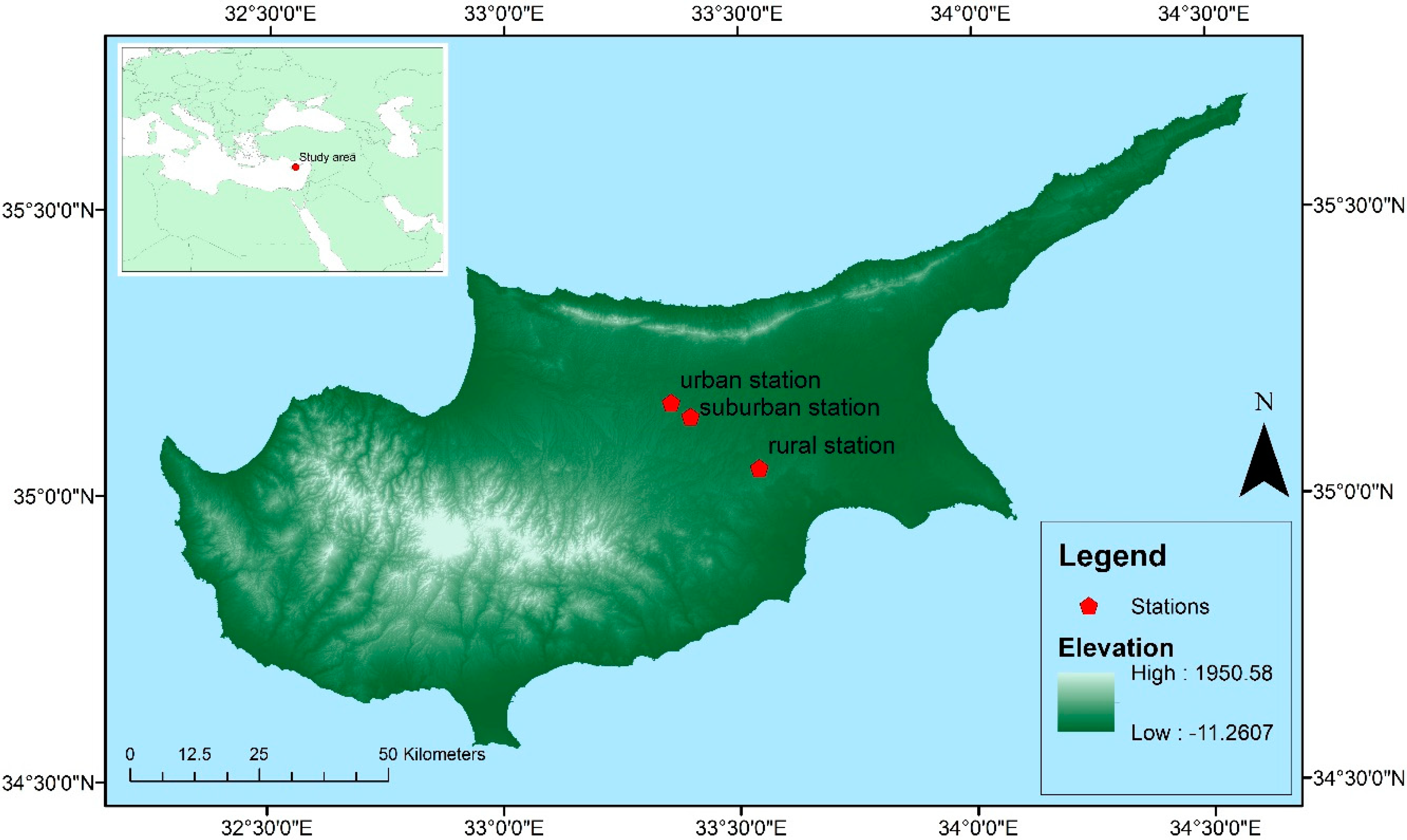
Cyprus (Figure 1) is an island in the eastern basin of the Mediterranean Sea with an area of 9251 km². Cyprus has a hot summer Mediterranean climate and a hot semi-arid climate (in the northeastern part of island) according to Köppen climate classification signs Csa (Mediterranean hot summer climates) and BSh (Hot semi-arid climates) [24], with warm to hot dry summers and wet winters. The hot, dry summer lasting from May to September is affected by the low barometric centered in Southwest Asia, which contributes to the persistence of high temperatures and low precipitation levels.

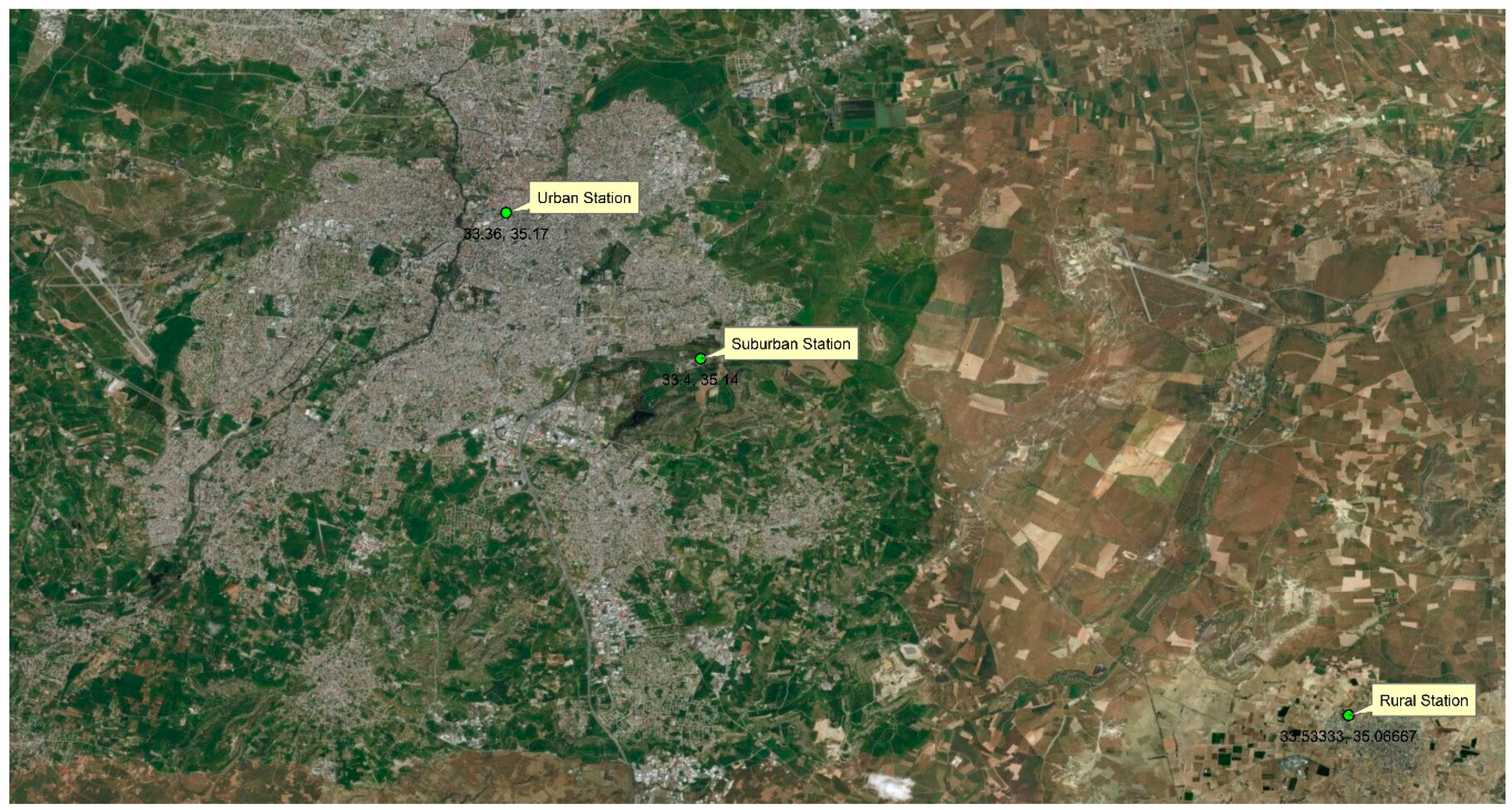
Three meteorological stations were investigated: an urban station (35.17° N, 33.36° E) in the city center, a suburban station (35.15° N, 33.40° E), and a rural station (35.05° N, 33.54° E) at a distance of 21.3 km from the urban station (Figure 1). The urban, the suburban, and the rural stations are located at altitudes 160, 162, and 175 m above mean sea level, respectively (Figure 2). The maximum height of buildings is 24 m (six floors) at the urban area, 17 m (four floors) at the suburban area, and 8.3 m (two floors) at the rural area [25].

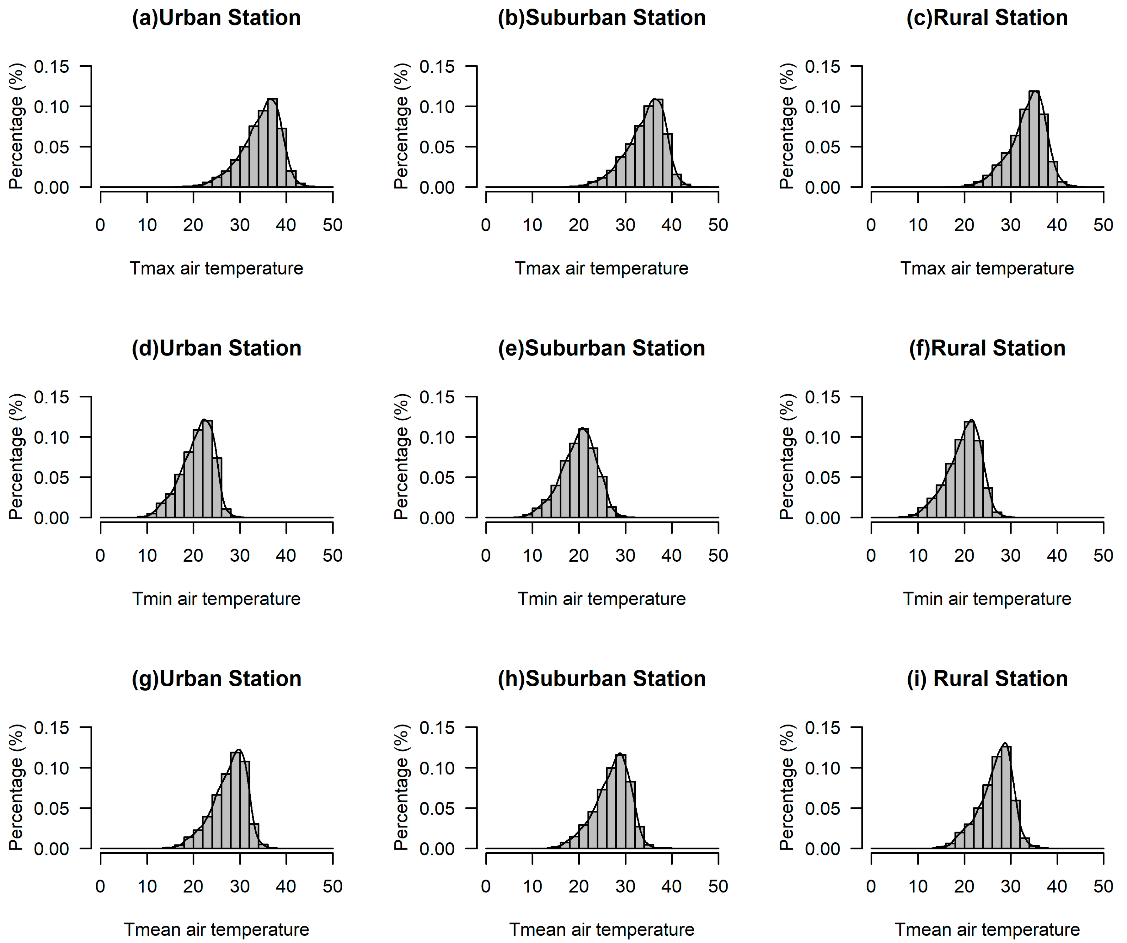
The daily ambient air temperature (mean, maximum, and minimum) as well as the daily accumulated precipitation were obtained from the Meteorological Service of Cyprus for the period 1988–2017 (inclusive) [26]. Only the months April to September were chosen from the continuous dataset for further investigation. No outliers or missing data existed in the final dataset, ensuring normality and homogeneity of variance throughout the series. The mean ambient air temperatures for the months May to September were 27.6 °C, 27.1 °C, and 26.7 °C for the urban, the suburban, and the rural areas, respectively.

3. Methodology

3.1. Ambient Air Temperatures and Total Precipitation in the Urban, Suburban and Rural Areas

For the investigated years (1988–2017), a linear trend analysis was used to estimate the statistical significance of the slope (b) of trend lines and reveal specific patterns of the local climate of the monthly values of temperatures and precipitation for months April to September for the three stations. The t-test analysis was used to allow for comparisons with other studies that investigate increasing and decreasing trends of temperature, precipitation, and climatic abnormalities [27,28,29,30]. According to the t-test analysis (

Table 1. t-test (t_b values) for testing the significance of the slope of trend lines.

	Urban	Suburban	Rural
Tmax (°C)	0.745	1.344	1.452
Tmin (°C)	5.576	8.813	8.284
Tmean (°C)	3.006	5.134	4.428
Total precipitation (mm)	−1.712	1.158	0.112

) for the regression lines, the maximum air temperatures showed a steady profile throughout the years (values less than 2.048 for α = 0.05 and 28d.f), but the minimum and the mean temperatures showed a statistically increasing trend (values over than 2.048 for a = 0.05 and 28d.f).

The following table (

Table 2. Average monthly maximum (Tmax), minimum (Tmin), and mean (Tmean) air temperatures (and daily absolute maximum and minimum ambient air temperatures) and total precipitation using data from years 1988–2017 for urban, suburban, and rural stations.

		May	June	July	August	September
Tmax (°C)	Urban	29.9 [17.5–41.1]	34.4 [17.7–44.9]	37.4 [25.4–44.8]	37.2 [27.9–44.5]	33.6 [23.9–41.9]
	Suburban	29.5 [18.1–41.5]	34.2 [23.7–45.4]	37.2 [29.7–43.6]	37.1 [30.2–46.2]	33.5 [24.4–41.1]
	Rural	29.1 [18.0–41.0]	33.4 [23.3–42.5]	36.2 [29.7–44.5]	36.1 [30.0–43.0]	33.0 [25–42.2]
Tmin (°C)	Urban	16.2 [9.2–23.2]	20.5 [12.3–29.1]	23.5 [17.0–29.4]	23.4 [18.8–29.7]	20.2 [13.8–27.0]
	Suburban	15.3 [7.4–23.7]	19.8 [10.2–28.7]	22.6 [15.5–30.2]	22.6 [16.3–30.1]	19.4 [13.0–26.9]
	Rural	15.2 [6.8–24.4]	19.5 [12.0–29.5]	22.5 [16.0–29.8]	22.6 [16.5–29.1]	19.6 [13.1–27.4]
Tmean (°C)	Urban	23.0 [14.5–31.0]	27.5 [16.6–35.6]	30.4 [24.1–36.1]	30.3 [24.5–36.2]	26.9 [19.8–34.0]
	Suburban	22.4 [14.3–31.0]	27.0 [17.0–35.7]	29.9 [23.0–36.3]	29.8 [24.4–38.2]	26.4 [19.5–33.6]
	Rural	22.1 [14.3–32.0]	26.4 [19.0–35.8]	29.4 [23.5–36.6]	29.3 [24.8–35.9]	26.3 [19.6–34.8]
Total Precipitation (mm)	Urban	18.9	7.0	3.7	2.4	4.5
	Suburban	24.8	13.8	4.6	1.6	11.5
	Rural	26.8	14.0	2.7	1.4	10.1

) presents mean monthly maximum, minimum, and mean air temperatures and the total monthly precipitation for the three investigated areas (urban, suburban, and rural) for months May to September. The highest average monthly temperatures developed in July, followed by August for all areas. Precipitation was the lowest in August with values close to zero. Moreover, the histograms (Figure 3a–i) show the distribution of these reference values.

Figure 3 shows the percentage distribution of daily mean, maximum, and minimum temperatures for the three investigated areas. According to the percentage values of Figure 3, the maximum daily values of months May until September were observed at the urban and the suburban stations with values of 36–38 °C appearing more frequently (highest percentage), whereas at the rural station, values of 34–36 °C appeared more frequently (Figure 3). The minimum daily temperatures appeared slightly increased at the urban station with values between 22–24 °C, whereas at the other two stations, they were lower and fairly equal (Table 2) with values 20–22 °C (Figure 3). The mean daily temperatures of May until September ranged mainly between 28–30 °C for all stations, but a closer investigation showed a steady decrease of 0.5 °C during the thirty investigated years.

The mean monthly total precipitation was usually lower at the urban station during the months May, June, and September, whereas for the months July and August, due to the extremely low precipitation levels (Table 2), a significant variation between the three stations could not be corroborated.

3.2. Temperature Anomalies

The term temperature anomaly (Tanomaly) means a deviation from a long-term average, with positive/negative Tanomaly values indicating that the observed temperature was warmer/cooler than the reference value. Reference values were computed on local scales over a defined time period, establishing a baseline from which the anomalies were calculated. This resulted in normalization of the data in order for them to be compared and combined to a more accurate temperature pattern with respect to normal climatic values of a specific region. The average maximum temperatures of each month (Tmax of Table 2) were considered as the baseline values from which anomalies were calculated and were used for the calculation of temperature anomalies.

3.3. Standardized Precipitation and Evapotranspiration Index (SPEI)

Droughts are identified by their effect at different levels, such as duration, intensity, magnitude, spatial extent, and onset, but there is not a physical variable to quantify them. Over the years, several drought indices have been developed with the most wide usage of the Palmer Drought Severity Index (PDSI) [31,32] and the Standardized Precipitation Index (SPI) [33,34]. PDSI is based on a simplified water balance equation that incorporates prior precipitation, moisture supply, runoff, and evaporation demand at the surface level [32], whereas SPI is based on precipitation anomalies and has the advantage of analyzing different temporal scales [33].

In this study, we utilized the Standardized Precipitation and Evapotranspiration Index (SPEI), which is a commonly used index that combines the sensitivity of PDSI with changes in evaporation demand and the multi-temporal nature of the SPI [35]. Several studies showed that SPEI more accurately captures the impacts of droughts on hydrological, agricultural, and ecological variables compared to SPI or PDSI. The SPEI allows comparison of drought severity through time and space since it can be calculated over a wide range of climates and is statistically robust with clear and comprehensible calculation procedure [35,36,37].

The following table (

Table 3. Categorization according to the Standardized Precipitation-Evapotranspiration Index (SPEI) values.

SPEI Values	Categories
Over 2	Extreme Wet
1.5 to 2	Severe Wet
1 to 1.5	Moderate Wet
−1 to 1	Normal climate
−1.5 to −1	Moderate Dry
−2 to −1.5	Severe Dry
Less than −2	Extreme Dry

) shows the categorization of the area according to SPEI values. The SPEI allows the comparison of drought severity through time and intensity and can identify the onset and the end of drought episodes. For the calculation of SPEI, the preceding month’s precipitation is required for the water balance equation. SPEI was calculated on a daily basis in order to relate drought episodes to soil water content and river discharge in headwater areas. Larger time scales are used to monitor drought conditions in different hydrological subsystems, such as reservoir and groundwater storages [38].

The SPEI index was calculated based on precipitation and potential evapotranspiration (PE), which was evaluated according to the SPEI package [36] in RStudio by implementing the Hargreaves equation and the log-logistic distribution of the water surplus or deficit. The Hargreaves equation [39] was preferred over other equations of potential evapotranspiration (Penman or Thornthwaite) due to its simplicity and accuracy, as it gives an estimate of the potential evapotranspiration based mainly on temperature adjusted for the sunshine hours per day and is given by:

$$PE=0.0023·\left(Tmean+17.8\right)·{\left(Tmax-Tmin\right)}^{0.5}·R_a$$

(1)

where Tmean, Tmax, and Tmin are mean, maximum, and minimum daily temperatures (Celsius), respectively, and Ra is the extra-terrestrial radiation (MJm⁻²day⁻¹), which is calculated as:

$${\mathrm{R}}_{\mathsf{\alpha }}=\frac{1440}{\mathsf{\pi }}·0.082·(1+0.033·\cos \left(\frac{2\mathsf{\pi }·\mathrm{Julian}\mathrm{day}}{\mathrm{Number}\mathrm{of}\mathrm{days}\mathrm{in}\mathrm{year}\left(366\mathrm{in}\mathrm{leap}\mathrm{year}\right)}\right))$$

(2)

A simple measure of the water surplus or deficit for each analyzed day (Di) is then calculated as the difference between the precipitation (PR) and the PE of each day.

$$D_i=P{R}_i-P{E}_i$$

(3)

Vicente-Serrano et al. [35] further explored this water surplus or deficit at different time scales, adjusted it to a log-logistic probability distribution [F(D)], and proposed the climatic drought index SPEI [35].

According to Vicente-Serrano et al. [35], the standardized values of the log-logistic probability distribution [F(D)] and the soil water balance (W) values could be used for the SPEI calculation by following the classical approximation of Abramowitz and Stegun [40] and resulted in the following equation:

$$SPEI=W-\frac{C_0+C_{1}W+C_2{W}^2}{1+d_{1}W+d_2{W}^2+d_3{W}^3}$$

(4)

where the constants are C₀ = 2.515517, C₁ = 0.802853, C₂ = 0.010328, d₁ = 1.432788, d₂ = 0.189269, and d₃ = 0.001308. The average value of the SPEI is 0, and the standard deviation is 1. For this study, daily SPEI index was evaluated using the data of the investigated time period (years 1988–2017) for the three stations.

3.4. Retrospective Approach with Cross Correlation

Soil moisture is increased with precipitation, and this consequently modifies the total energy used by latent heat flux. Therefore, more energy is available for sensible heating, resulting in the increase of ambient air temperature [15]. The effects of precipitation may prolong for a number of days and may vary according to the investigated area. The lag period of the precipitation effect on lowering daily temperatures was found using the cross correlation function (CCF analysis), which computes the correlation between two variables, x and y. If ⊗ denotes correlation, then the cross-correlation function is defined as [41]:

$${\mathrm{R}}_{\mathrm{xy}}\left(\mathrm{t}\right)=\mathrm{x}\left(\mathrm{t}\right)\otimes \mathrm{y}\left(\mathrm{t}\right)={\int }_{-\infty }^{\infty }\mathrm{x}\left(\mathrm{h}\right)\mathrm{y}\left(\mathrm{t}+\mathrm{h}\right)\mathrm{dh}$$

(5)

where y(t) are the precipitation levels shifted to the left by h-lag time, and x(t) is the temperature anomalies deviating from the average maximum temperatures of each month (Tmax of Table 2). The lag period used in our study was h = 0, 1, 2, …, 30 days, thus we also had to employ daily precipitation levels in the month of April.

The cross-correlation analysis was also followed for correlating the temperature anomalies [x(t) component] with the SPEI [y(t) component]. The same lag period h = 0, 1, 2, …, 30 days was used. The variances of the cross-correlation coefficient under the null hypothesis of zero correlation for both cross-correlation analyses were approximately 0.0002.

4. Results

4.1. Temperature Anomalies and Lag Period

In Section 3.1, the average maximum temperatures of each month were found (Tmax of Table 2) and were later used for the calculation of the temperature anomalies for the months May to September. These anomalies were divided into positive (above the average) or negative (below the average) values with the majority of them varying between −2 °C and 2 °C (as shown in Figure 4). Specifically, for months May to September and years 1988–2017 (inclusive), around 52.6%, 53.6%, and 56.7% of the temperature anomalies in the urban, the suburban, and the rural stations, respectively, varied between −2 °C and 2 °C. The most positive anomalies were found at the suburban station, and the most negative anomalies were found at the rural station. Moreover, about 2.6–3% of the temperature extremes exceeded the average monthly maximum temperature by 6 °C at all stations.

Figure 5 illustrates the results of the cross correlation analysis (Section 3.4) for the temperature anomalies happening after a precipitation event for the three investigated areas. The blue dashed lines in Figure 5 represent the significance limit at α = 0.05 of R_xy(t) (Equation (5)) in order to determine the statistical significance of a null-hypothesis. The variance of the cross-correlation coefficient under the null hypothesis of zero correlation for this study was approximately 0.0002, thus the approximate critical values (at the 5% level) were ±0.029 (to three decimal places). On a rainy day, day 0, an immediate drop of temperature appeared, which prolonged for six, seven, and nine days at the urban, the suburban, and the rural stations, respectively. The rural station was influenced by precipitation, resulting in a delayed increase of temperature after a rainfall event, which explained the higher percentage of negative anomalies as well as the relatively steady temperature profile without any extremities. Negative temperature anomalies prolonged for up to nine days at the rural station, signifying the importance of soil moisture for preventing extremely high temperatures in the summer. On the contrary, the urban station seemed the most susceptible to extremely high temperatures above the average maximum temperatures of each month (Tmax of Table 2), with the most days over 4 °C above the average maximum temperatures of each month. In urban areas, the urban environment resulted in high water runoff through the concrete structures and rapid evaporation of the overlay water, leading to a small decrease of temperature that only lasted for five to six days. He et al. [42] also indicated stronger impacts on diurnal temperature range extremes from short-term rather than long-term precipitation deficits and that low soil moisture due to precipitation deficits increase air temperatures through higher sensible heat flux [42].

The cross-correlation analysis of SPEI with temperature anomalies revealed the stronger relationship and the importance of this index. The correlation coefficient increased from −0.2 for precipitation to −0.5 for SPEI, a percentage increase of 150%. Temperature anomalies and SPEI had a negative correlation and evolved concurrently, i.e., when one parameter increased, the other decreased, and vice versa. In the case of SPEI with regards to temperature anomalies, the lag period was significantly longer: 15, 11, and 16 days at the urban, the suburban, and the rural stations, respectively.

Figure 6 shows the time-series variation of daily temperature anomalies with respect to the daily accumulated precipitation. Negative temperature anomalies were clearly observed for a rainy day, as well as for the days following a precipitation event, suggesting local climatic variations strongly controlled by the evapotranspiration of small soil moisture after the precipitation event. From Figure 6, it was also noted that there was no significant trend towards increasing or decreasing temperature anomalies in Cyprus within the last 30 years during the summer period. In contrast, temperatures showed some changes over time, with average and minimum temperatures increasing, and this was accompanied by a significant decrease in the daily temperature range (DTR) [9].

Precipitation is directly linked to regional evapotranspiration, but this is trivial in cases of intense precipitation or areas under extreme drought. In the investigated areas of this study, moderate drought conditions dominated, thus it was expected that, after rainfall, the higher soil moisture would increase the evapotranspiration. Positive soil moisture anomaly led to a negative temperature anomaly mediated through a positive anomaly of evapotranspiration. Small soil moisture indicated a small evapotranspiration rate, which, according to Seneviratne et al. [15], is stronger in transitional zones between dry and wet climates. In the case of precipitation, the soil moisture may increase, leading to an evapotranspiration rate increase and a consequent decrease of temperature and negative temperature anomalies. Typically, low evapotranspiration rate is linked to lower energy used by latent heat flux and an increase in sensible heat flux and thus an increase in positive temperature anomalies. Therefore, even a small increase of the evapotranspiration rate after a precipitation event suggested higher energy used by latent heat rather than sensible heat flux, leading to fewer positive temperature anomalies compared to days not following a precipitation event.

4.2. Analysis of SPEI

The SPEI was calculated for years 1988–2017 for the months of May to September based on the temperatures and the precipitation of the preceding days. The regression lines of

Table 4. Monthly mean and standard deviation (sd) values of SPEI and temperature anomalies (T_anomaly) for urban, suburban, and rural station.

Month		Urban	Suburban	Rural
May	Tanomaly (mean ± sd)	−0.002 ± 4.20	0.046 ± 4.01	−0.007 ± 3.82
	SPEI (mean ± sd)	0.25 ± 0.74	0.31 ± 0.69	0.30 ± 0.72
June	Tanomaly (mean ± sd)	0.011 ± 3.27	−0.048 ± 3.19	−0.031 ± 3.04
	SPEI (mean ± sd)	−0.39 ± 0.58	−0.37 ± 0.57	−0.37 ± 0.59
July	Tanomaly (mean ± sd)	−0.045 ± 2.40	−0.034 ± 2.20	0.045 ± 2.17
	SPEI (mean ± sd)	−0.913 ± 0.54	−0.943 ± 0.46	−0.925 ± 0.51
August	Tanomaly (mean ± sd)	0.040 ± 2.08	0.025 ± 2.02	−0.011 ± 1.93
	SPEI (mean ± sd)	−0.93 ± 0.43	−0.989 ± 0.42	−0.931 ± 0.45
September	Tanomaly (mean ± sd)	0.001 ± 2.83	0.021 ± 2.76	0.027 ± 2.49
	SPEI (mean ± sd)	−0.316 ± 0.55	−0.309 ± 0.58	−0.358 ± 0.54

show the existence of a negative relationship between the parameters SPEI and Tanomalies. They could not be used for the estimation of the daily variation of Tanomalies, as there was large variation around the mean values and the respective standard deviations of the two parameters (SPEI and Tanomalies). A statistically significant increasing trend for the time-series of the mean values of mean and minimum ambient air temperatures (Table 1) was previously proven. However, the regression lines of Table 4 reveal the higher decreasing trend of SPEI during the thirty investigated years at the suburban and the rural station, which was probably attributed to by external factors (change of land cover, meteorological conditions, etc.). More frequent temperature anomalies were observed in August for the urban and the suburban stations and in July for the rural station.

According to Figure 7, the urban, the suburban, and the rural stations were mainly characterized by a normal climate (SPEI between −1 to 1) with 73.5%, 73.9%, and 74.2% SPEI values, respectively, for the five months. The highest percentages (77.6 to 86.9%) of normal climatic conditions (SPEI between −1 and 1) were observed in May, June, and September.

As depicted in Figure 7, July and August were the major drought months in the study area with SPEI below −1, contributing to about 35% of the total SPEI values. It is worth noting that, during July and August, no days were observed with wet conditions (SPEI over 1), whereas in May, a small occurrence of wet conditions (SPEI over 1) associated with negative Tanomalies was observed at a percentage of 13.4–14.5% (Figure 7 and

Table 5. Percentage of occurrence of T_anomalies for each station under wet conditions (SPEI > 1), dry conditions (SPEI < −1), and normal climatic conditions (−1 < SPEI < 1).

May
	Urban			Suburban			Rural
	SPEI < −1	SPEI > 1		SPEI < −1	SPEI > 1		SPEI < −1	SPEI > 1
Τanomaly > 0	7.3%	0.5%	Τanomaly > 0	5.3%	0.4%	Τanomaly > 0	5.2%	0.6%
Τanomaly < 0	0.2%	14.3%	Τanomaly < 0	0.1%	13.4%	Τanomaly < 0	0.1%	14.5%
all Τanomaly	−1 < SPEI < 1	77.6%	all Τanomaly	−1 < SPEI < 1	80.8%	all Τanomaly	−1 < SPEI < 1	79.6%
June
	Urban			Suburban			Rural
	SPEI < −1	SPEI > 1		SPEI < −1	SPEI > 1		SPEI < −1	SPEI > 1
Τanomaly > 0	12.6%	0%	Τanomaly > 0	11.2%	0%	Τanomaly > 0	11.2%	0.1%
Τanomaly < 0	2.3%	1.4%	Τanomaly < 0	2.1%	1.0%	Τanomaly < 0	2.2%	1.8%
all Τanomaly	−1 < SPEI < 1	83.8	all Τanomaly	−1 < SPEI < 1	85.7%	all Τanomaly	−1 < SPEI < 1	84.7%
July
	Urban			Suburban			Rural
	SPEI < −1	SPEI > 1		SPEI < −1	SPEI > 1		SPEI < −1	SPEI > 1
Τanomaly > 0	29.5%	0%	Τanomaly > 0	29.7%	0%	Τanomaly > 0	28.7%	0%
Τanomaly < 0	12.4%	0%	Τanomaly < 0	13.3%	0%	Τanomaly < 0	15.5%	0%
all Τanomaly	−1 < SPEI < 1	58.2%	all Τanomaly	−1 < SPEI < 1	57.0%	all Τanomaly	−1 < SPEI < 1	55.8%
August
	Urban			Suburban			Rural
	SPEI < −1	SPEI > 1		SPEI < −1	SPEI > 1		SPEI < −1	SPEI > 1
Τanomaly > 0	32.0%	0%	Τanomaly > 0	33.7%	0%	Τanomaly > 0	27.4%	0%
Τanomaly < 0	12.3%	0%	Τanomaly < 0	15.3%	0%	Τanomaly < 0	15.2%	0%
all Τanomaly	−1 < SPEI < 1	55.7%	all Τanomaly	−1 < SPEI < 1	51.1%	all Τanomaly	−1 < SPEI < 1	57.4%
September
	Urban			Suburban			Rural
	SPEI < −1	SPEI > 1		SPEI < −1	SPEI > 1		SPEI < −1	SPEI > 1
Τanomaly > 0	10.1%	0%	Τanomaly > 0	10.1%	0%	Τanomaly > 0	10.3%	0%
Τanomaly < 0	1.0%	1.0%	Τanomaly < 0	0.7%	1.2%	Τanomaly < 0	1.1%	0.3%
all Τanomaly	−1 < SPEI < 1	87.9%	all Τanomaly	−1 < SPEI < 1	88.0%	all Τanomaly	−1 < SPEI < 1	88.2%

).

Dry conditions with SPEI lower than −1 were associated with positive temperature anomalies (Tanomalies > 0 °C) at percentages from 10.7 to 31.7%. Dry conditions were associated with negative temperature anomalies (Tanomalies < 0 °C) at percentages from 1.4 to 15.4% (Table 5). This frequency was increased in July and August, confirming the overall drought in the area during these two summer months.

In summary, there were no large discrepancies in the monthly SPEI values between the three areas, but more severe and extreme dry conditions (SPEI less than −1.5) occurred at the rural area in July and August.

To quantitatively describe the SPEI, we calculated the percentage of positive and negative temperature anomalies for SPEI lower than −1 (drought conditions) and higher than 1 (wet conditions). The results are shown in Table 5. In May, the percentage of negative temperature anomalies with SPEI > 1 was greater than the percentage of positive anomalies combined with either SPEI < −1 or SPEI > 1, indicating a greater proportion of low temperatures occurred under wet conditions. For the months June to September, the percentage of positive temperature anomalies with SPEI < −1 was greater than the percentage of negative anomalies. Zero positive temperature anomalies were found for SPEI > 1 for months June to September, which indicated that all higher air temperatures occurred during dry conditions. No wet climatic conditions appeared during the summer, mainly due to the lack of precipitation. Positive temperature anomalies reached a peak in August under dry conditions, with occurrences of 32.0%, 33.7%, and 27.4% at the urban, the suburban, and the rural stations, respectively. Most of the temperature anomalies occurred for SPEI values between −1 and 1, with greater values in June and September. Comparison of the percentage values between the three stations revealed that most positive temperature anomalies occurred in the urban and the suburban areas, and most negative temperature anomalies occurred in the rural area.

4.3. Concurrent Drought and Hot Days

In the next stage, we investigated the occurrence of positive temperature anomalies above the average maximum temperatures of each month (Tmax of Table 2) with respect to the SPEI in order to assess whether they appeared more frequently under dry conditions. The regression analysis showed the monthly relation between the two variables—SPEI and temperature anomalies (T anomalies). The results according to Figure 8 and

Table 6. Linear regression analysis of temperature anomalies with respect to SPEI for the three stations and for the months May to September of the years 1988–2017, showing the regression equation (T_anomaly = A + B·(SPEI)), the t-test of the statistical significance of A and B, and the adjusted R² correlation coefficients.

Month	Station	A	B	tA	tB	R2
May	Urban	1.025	−4.127	10.17	−31.70	0.52
	Suburban	1.403	−4.417	14.86	−35.12	0.57
	Rural	1.108	−3.687	11.28	−29.14	0.47
June	Urban	−1.236	−3.220	−11.35	−21.09	0.33
	Suburban	−1.338	−3.535	−13.81	−24.61	0.40
	Rural	−1.139	−3.027	−11.79	−21.77	0.35
July	Urban	−2.338	−2.512	−18.27	−20.80	0.32
	Suburban	−2.572	−2.461	−17.86	−19.62	0.29
	Rural	−1.921	−2.127	−15.17	−17.76	0.25
August	Urban	−2.152	−2.339	−15.17	−17.03	0.24
	Suburban	−2.510	−2.563	−17.28	−18.94	0.28
	Rural	−1.878	−2.006	−14.65	−16.19	0.22
September	Urban	−1.128	−3.577	−14.45	−29.03	0.48
	Suburban	−1.025	−3.395	−13.92	−30.15	0.50
	Rural	−0.997	−2.865	−12.88	−24.06	0.39

and

Table 7. Paired t-test for the statistical significance between A_i.A_j and B_i.B_j (for t values greater than 1.96, the differences were statistically significant for α = 0.05).

	A			B
	Urban/Suburban	Urban/Rural	Suburban/Rural	Urban/Suburban	Urban/Rural	Suburban/Rural
May	1.057	1.160	0.189	1.598	−2.420	−4.087
June	0.833	0.721	−0.096	1.518	−0.935	−2.558
July	−0.821	−1.111	−0.361	0.337	−2.260	−2.506
August	−1.186	0.696	1.840	1.161	−1.801	−3.035
September	0.012	−1.294	−1.282	−1.092	−4.156	−3.236

showed:

■

R² values (Table 6) for SPEI and Tanomaly showed that there was an overall significant linear relationship between the two parameters, which varied from 0.2 to 0.57 (for more than 900 degrees of freedom) for each investigated area. These relatively low R² values are not uncommon in large datasets because the significance of the slope is due to the number of elements in the dataset.

■

Under normal climatic conditions (SPEI varying between −1 to 1) independent from the values of Tanomalies, we observed, for all the months, that the frequency of the pair SPEI/Tanomalies was generally the same at all stations (72.6% for urban, 72.5% for suburban, 73.1% for rural), representing a uniform climatic behavior in the wider range of Nicosia (Table 5).

■

Figure 8 and Table 6 portray the monthly temperature anomalies and their trends for different SPEI. Using a linear regression model, the rate of change was defined by the slope of the regression line and differed in each investigated area and month. The linear regression lines for months July and August were almost identical at all three stations with slopes −2.34 (July) and −2.51 (August) for the urban, −2.46 (July) and −2.56 (August) for the suburban, and −2.87 (July) and −3.03 (August) for the rural station. The linear regression line’s slope for May varied significantly with values −4.13, −4.42, and −3.69 for the urban, the suburban, and the rural stations, respectively, with higher occurrence of severe to moderate wet conditions (SPEI > 1) that were associated with positive as well as negative Tanomalies (Table 6).

■

The negative slope of the linear regression lines was larger in May (varying from −3.69 to −4.14) and smaller in July and August (varying from −2.01 to −2.56) at all three stations, confirming the larger effects of evapotranspiration and precipitation that existed during the months March to April on the values of Tanomalies for the month of May.

■

With the use of t-test analysis, the absolute values of |t_A| and |t_B| were calculated in order to check the statistical significance of A and Β coefficients of the linear regression lines with:

$$T_{anomaly}=A+B·SPEI$$

(6)

According to Table 6, for all cases, the coefficients A and B were found to be statistically significant (bold values) with |t_A| > t_0.05 = 1.96 and |t_B| > t_0.05 = 1.96.

■

Paired samples t-test was employed to compare the mean difference in coefficients A and B between the different pairs of stations. The results are presented in Table 7 for the pairs urban/suburban, urban/rural, and suburban/rural for all months. Statistically significant mean difference was obtained (t > 1.96; α < 0.05) at 95% level of significance. The results showed that the coefficient A was considered statistically equal for all pairs, indicating that the three investigated areas were nearby. The coefficient B defined the slope of the linear regression lines, which was a different trend of variation between the time series and suggested that external factors (land cover, meteorological conditions, etc.) differently affected the three stations during the thirty investigated years. The coefficient B was considered statistically equal (t_i,j < 1,96) in all the investigated months for the pair urban/suburban. For the pair urban/rural for months May, July, and September, the t-test was considered statistically significant. For the pair suburban/rural, the t-test showed that the B coefficients were statistically significant for all the months, which was attributed to a faster development of construction in the suburban area in relation to the urban area when both were compared to the rural area.

■

The regression lines that were determined (Table 6 and Figure 8) only showed the existence of a negative relationship between the parameters SPEI and Tanomaly, but they could not be used for the estimation of the daily value of Tanomaly.

5. Discussion and Conclusions

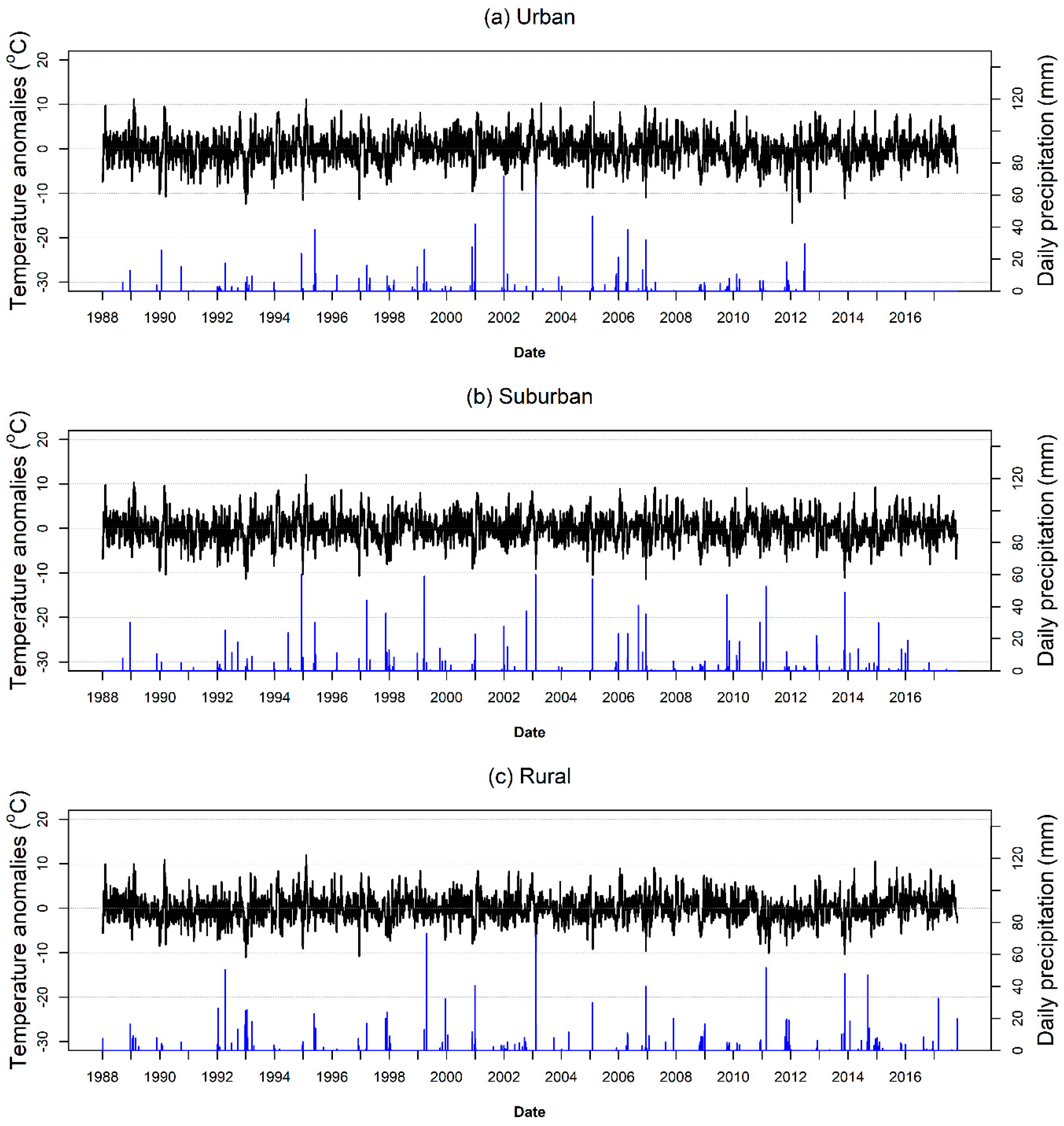
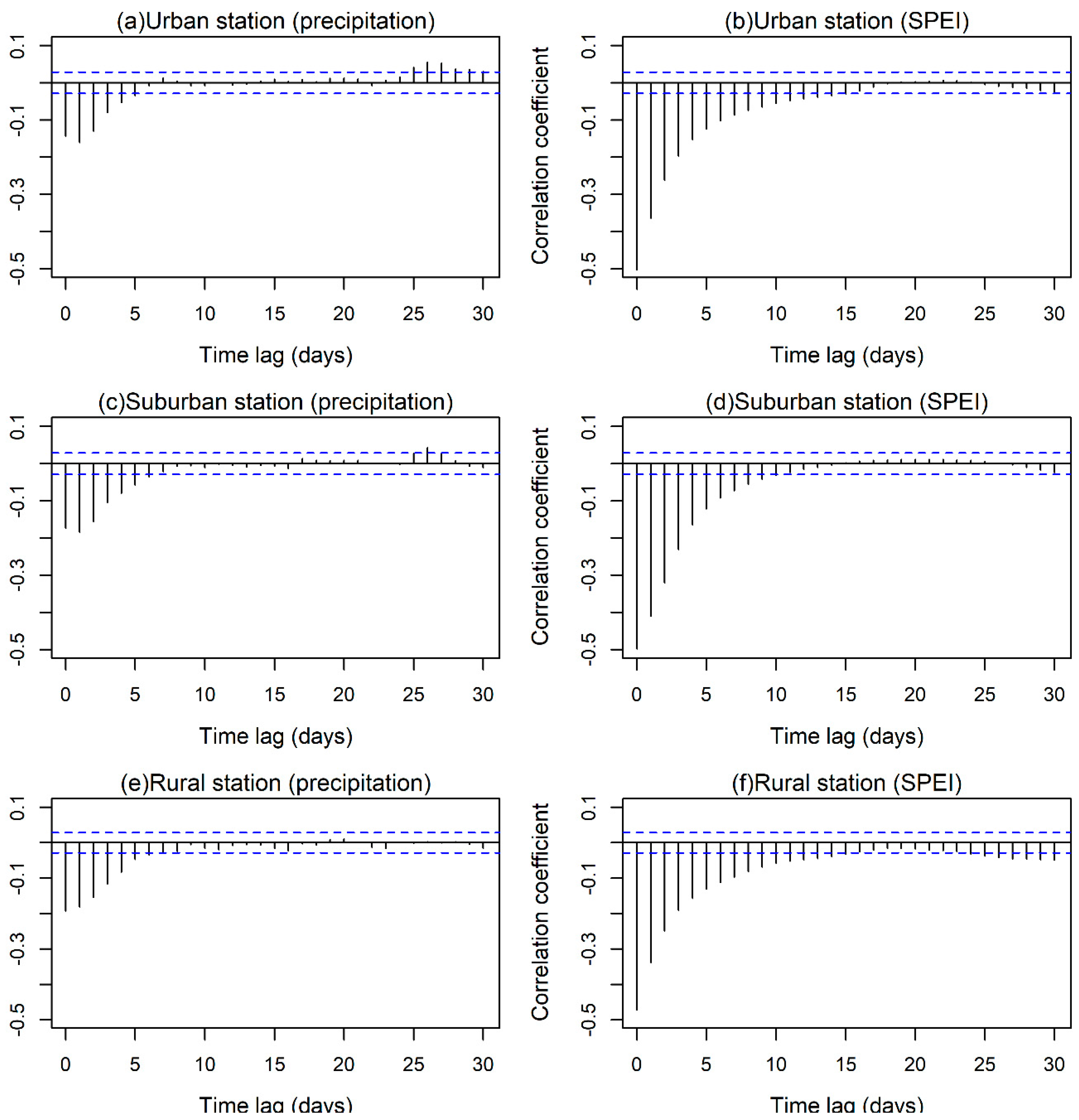
Through linear and cross-correlation statistical analysis, this study examined the compound effect of precipitation levels and evapotranspiration rates of the preceding days to summer temperature anomalies for years 1988–2017. The observations of the time-series figure (Figure 6) and the cross-correlation results showed that the cooling effect of precipitation was higher and lasted more in rural and suburban areas compared to urban areas, a fact directly related to the evaporation potential of the area concerned. We showed that precipitation was the dominant driving force of positive temperature anomalies and that varying evapotranspiration rates contributed to the development of moderate to severe drought in the investigated areas.

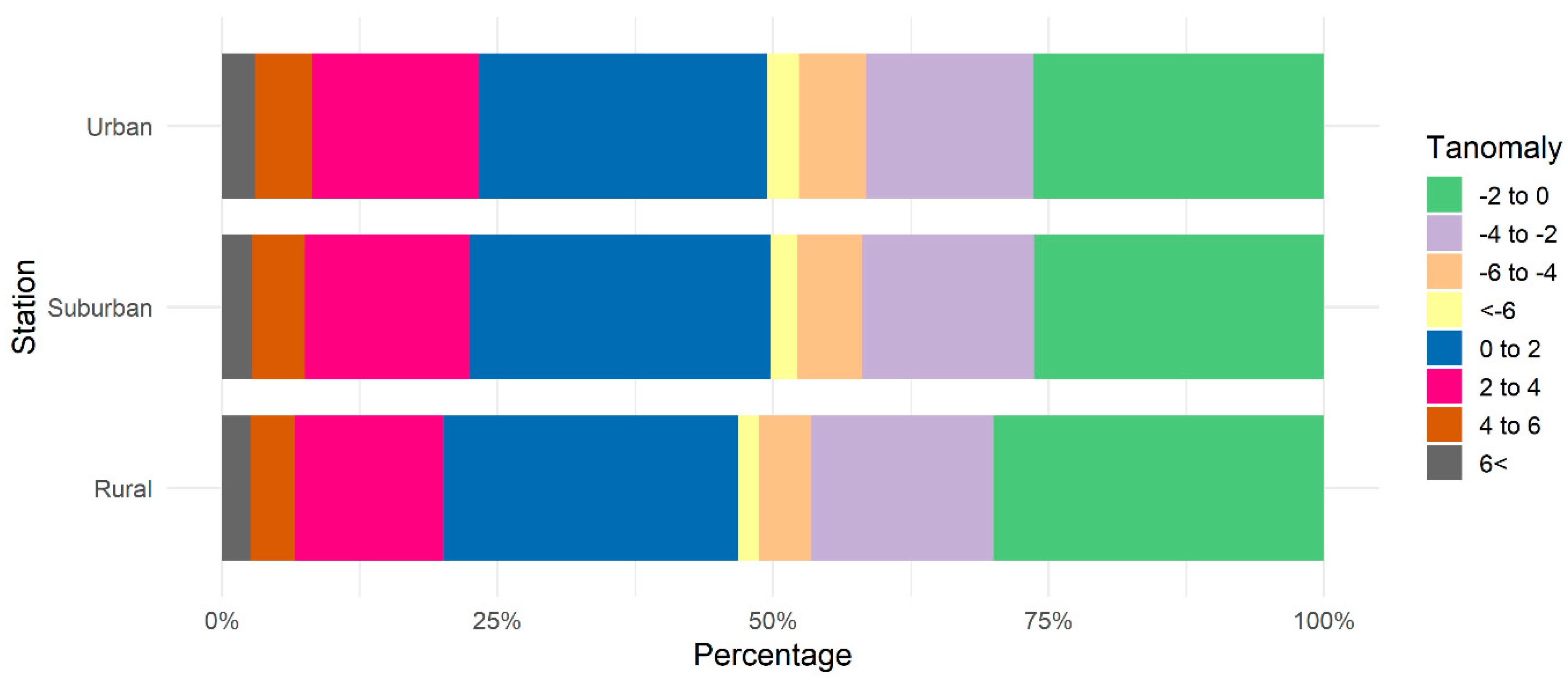
Particularly, the investigation of temperature anomalies showed a higher correlation for the concurrent month’s precipitation compared with precipitation in the preceding months, suggesting that moisture was depleted faster. This showed that there was a lag effect of soil moisture memory of six, six, and nine days in the urban, the suburban, and the rural areas, respectively. In warmer areas (urban and suburban areas), the larger evaporative demand from the atmosphere exacerbated the existing drought conditions and its impacts. Also, the higher urban and suburban temperatures (Table 2) compared to the rural area could significantly reduce the natural storage of water. With view of the precipitation events, the negative temperature anomalies suggested local climatic variations strongly controlled by the evapotranspiration of small soil moisture after the precipitation event. The SPEI was later used that employed both precipitation and evapotranspiration rates to characterize dry or wet conditions. The cross-correlation analysis of SPEI with temperature anomalies revealed the stronger relationship with negative correlation coefficient of −0.5 and highlighted the importance of this index. In the case of SPEI with regards to temperature anomalies, the lag periods according to the cross-correlation analysis were significantly longer: 15, 11, and 16 days at the urban, the suburban, and the rural stations, respectively. The higher surface albedo of the urban infrastructure may have led to additional warming. This does not necessarily translate to drier conditions and longer droughts, but it creates challenges for better water reservoir management.

According to this study, the SPEI has a high correlation with temperature anomalies and may be considered as a key tool for the identification of abnormal weather conditions and extremely high temperatures. 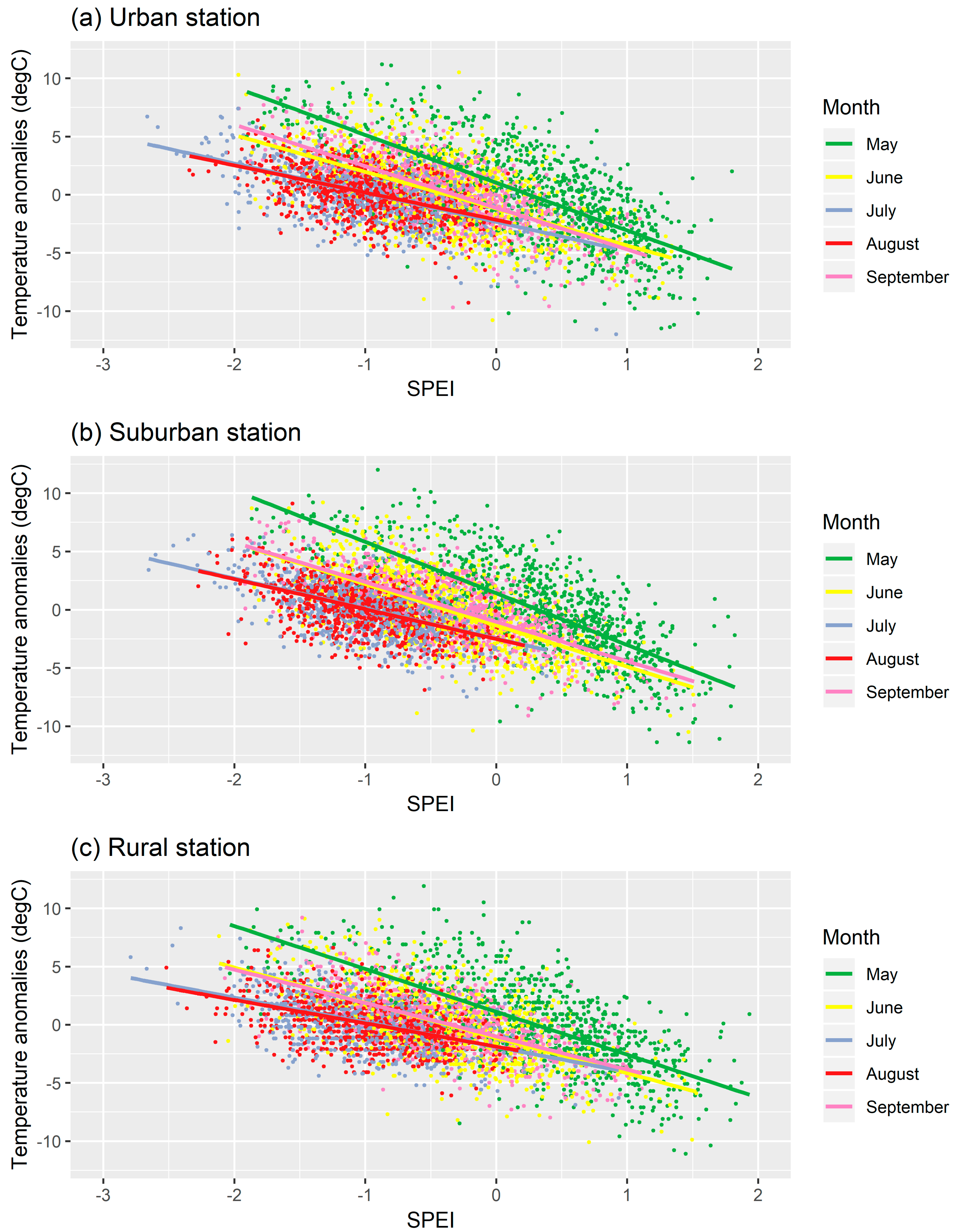Moreover, it confirmed that rainfall events combined with evapotranspiration, which could be effectively represented by SPEI index variation, may be the main regulators of soil moisture rather than the amount of monthly rainfall [43,44]. In the results section, the temperature anomalies were inversely correlated with precipitation anomalies, and the SPEI index and the linear regression coefficients were found. High temperatures during the summer months may be understood by the investigation of the soil moisture to understand the impact of soil storage memory on ambient air temperatures. Further analysis could focus on the division of temperature anomalies based on the amount of rainfall as well as the intervals between rainfall events. We should consider the effects of not only precipitation but also evapotranspiration in future studies to better understand the length of extreme weather conditions.

Further analysis focused on the statistical investigation of the linear regression lines of the SPEI with temperature anomalies for the three stations and for each month. The results of the paired t-test for the statistical significance showed that the coefficients A of Table 7 were considered statistically equal between them for all pairs, indicating that the three investigated areas were nearby. The B coefficients suggested that external factors (land cover, meteorological conditions, etc.) differently affected the three stations during the thirty investigated years. This study focused on the analysis of the effect of precipitation during the summer period on temperatures and particularly the deviation of temperature from the mean monthly value. The spatial investigation revealed a similar climatic profile in all three investigated areas but showed a noteworthy different lag effect of precipitation. Particularly, precipitation in rural areas led to a longer decrease of temperature compared to the urban and the suburban areas because the wet ground favored the increased evapotranspiration and the decrease of sensible heat flux. Later, the investigation of SPEI further supported the above statement, because SPEI was strongly negatively correlated with positive temperature anomalies.

Future work should focus on the effect of the intervals between precipitation events in urban, suburban, and rural areas. In this study, the semi-arid climate in Cyprus and the infrequent precipitation allowed a more comprehensive understanding of the lag effect of precipitation during the dry period (summer) in areas with different land cover. The lag period may vary seasonally; therefore, further investigation during the winter is necessary. The investigation of the transitional phase of dry and wet climates in Cyprus will likely confirm the strong soil-moisture climate coupling, which is the strong dependency of evapotranspiration on soil moisture during the dry periods and the little impact of soil moisture on evapotranspiration during the wet periods.

References

1. Yiou, P.; Vautard, R.; Naveau, P.; Cassou, C. Inconsistency between atmospheric dynamics and temperatures during the exceptional 2006/2007 fall/winter and recent warming in Europe. Geophys. Res. Lett. 2007, 34, 1–7. [Google Scholar] [CrossRef]
2. Fischer, E.M.; Seneviratne, S.I.; Vidale, P.L.; Lüthi, D.; Schär, C. Soil moisture-atmosphere interactions during the 2003 European summer heat wave. J. Clim. 2007, 20, 5081–5099. [Google Scholar] [CrossRef]
3. Miralles, D.G.; Gentine, P.; Seneviratne, S.I.; Teuling, A.J. Land–atmospheric feedbacks during droughts and heatwaves: State of the science and current challenges. Ann. N. Y. Acad. Sci. 2019, 1436, 19–35. [Google Scholar] [CrossRef] [PubMed]
4. Cassou, C.; Terray, L.; Hurrell, J.W.; Deser, C. North Atlantic winter climate regimes: Spatial asymmetry, stationarity with time, and oceanic forcing. J. Clim. 2004. [Google Scholar] [CrossRef]
5. Feudale, L.; Shukla, J. Role of Mediterranean SST in enhancing the European heat wave of summer 2003. Geophys. Res. Lett. 2007. [Google Scholar] [CrossRef]
6. Doblas-Reyes, F.J.; García-Serrano, J.; Lienert, F.; Biescas, A.P.; Rodrigues, L.R.L. Seasonal climate predictability and forecasting: Status and prospects. Wiley Interdiscip. Rev. Clim. Chang. 2013, 4, 245–268. [Google Scholar] [CrossRef]
7. Trenberth, K.E.; Shea, D.J. Relationships between precipitation and surface temperature. Geophys. Res. Lett. 2005. [Google Scholar] [CrossRef]
8. LeMone, M.A.; Grossman, R.L.; Chen, F.; Ikeda, K.; Yates, D. Choosing the Averaging Interval for Comparison of Observed and Modeled Fluxes along Aircraft Transects over a Heterogeneous Surface. J. Hydrometeorol. 2003. [Google Scholar] [CrossRef]
9. Pyrgou, A.; Santamouris, M.; Livada, I. Spatiotemporal Analysis of Diurnal Temperature Range: Effect of Urbanization, Cloud Cover, Solar Radiation, and Precipitation. Climate 2019, 7, 89. [Google Scholar] [CrossRef]
10. Hirschi, M.; Seneviratne, S.I.; Alexandrov, V.; Boberg, F.; Boroneant, C.; Christensen, O.B.; Formayer, H.; Orlowsky, B.; Stepanek, P. Observational evidence for soil-moisture impact on hot extremes in southeastern Europe. Nat. Geosci. 2011, 4, 17–21. [Google Scholar] [CrossRef]
11. Vautard, R.; Yiou, P.; D’Andrea, F.; de Noblet, N.; Viovy, N.; Cassou, C.; Polcher, J.; Ciais, P.; Kageyama, M.; Fan, Y. Summertime European heat and drought waves induced by wintertime Mediterranean rainfall deficit. Geophys. Res. Lett. 2007, 34, 1–5. [Google Scholar] [CrossRef]
12. Seneviratne, S.I.; Lüthi, D.; Litschi, M.; Schär, C. Land-atmosphere coupling and climate change in Europe. Nature 2006, 443, 205–209. [Google Scholar] [CrossRef] [PubMed]
13. Vidale, P.L.; Lüthi, D.; Wegmann, R.; Schär, C. European summer climate variability in a heterogeneous multi-model ensemble. Clim. Chang. 2007, 81, 209–232. [Google Scholar] [CrossRef]
14. Rowell, D.P.; Jones, R.G. Causes and uncertainty of future summer drying over Europe. Clim. Dyn. 2006, 27, 281–299. [Google Scholar] [CrossRef]
15. Seneviratne, S.I.; Corti, T.; Davin, E.L.; Hirschi, M.; Jaeger, E.B.; Lehner, I.; Orlowsky, B.; Teuling, A.J. Investigating soil moisture-climate interactions in a changing climate: A review. Earth-Sci. Rev. 2010, 99, 125–161. [Google Scholar] [CrossRef]
16. McHugh, T.A.; Morrissey, E.M.; Reed, S.C.; Hungate, B.A.; Schwartz, E. Water from air: An overlooked source of moisture in arid and semiarid regions. Sci. Rep. 2015, 5, 13767. [Google Scholar] [CrossRef] [PubMed]
17. Wang, B.; Zha, T.S.; Jia, X.; Wu, B.; Zhang, Y.Q.; Qin, S.G. Soil moisture modifies the response of soil respiration to temperature in a desert shrub ecosystem. Biogeosciences 2014. [Google Scholar] [CrossRef]
18. Agam, N.; Berliner, P.R. Dew formation and water vapor adsorption in semi-arid environments—A review. J. Arid Environ. 2006, 65, 572–590. [Google Scholar] [CrossRef]
19. Liu, D.; Wang, G.; Mei, R.; Yu, Z.; Yu, M. Impact of initial soil moisture anomalies on climate mean and extremes over Asia. J. Geophys. Res. 2014, 119, 529–545. [Google Scholar] [CrossRef]
20. Naumann, G.; Alfieri, L.; Wyser, K.; Mentaschi, L.; Betts, R.A.; Carrao, H.; Spinoni, J.; Vogt, J.; Feyen, L. Global Changes in Drought Conditions Under Different Levels of Warming. Geophys. Res. Lett. 2018, 45, 3285–3296. [Google Scholar] [CrossRef]
21. Eliades, M.; Bruggeman, A.; Djuma, H.; Lubczynski, M. Tree Water Dynamics in a Semi-Arid, Pinus brutia Forest. Water 2018, 10, 1039. [Google Scholar] [CrossRef]
22. Feller, U.; Vaseva, I.I. Extreme climatic events: Impacts of drought and high temperature on physiological processes in agronomically important plants. Front. Environ. Sci. 2014, 2, 39. [Google Scholar] [CrossRef]
23. Pyrgou, A.; Santamouris, M. Increasing Probability of Heat-Related Mortality in a Mediterranean City Due to Urban Warming. Int. J. Environ. Res. Public Health 2018, 15, 1571. [Google Scholar] [CrossRef] [PubMed]
24. Peel, M.C.; Finlayson, B.L.; McMahon, T.A. Updated world map of the Koppen-Geiger climate classification. Hydrol. Earth Syst. Sci. 2007, 11, 1633–1644. [Google Scholar] [CrossRef]
25. Υπουργείο Εσωτερικών, Τ. Π. και O. Ισχύοντα Δημοσιευμένα Σχέδια Aνάπτυξης. Available online: http://www.moi.gov.cy/moi/tph/tph.nsf/page72_gr/page72_gr?OpenForm (accessed on 29 July 2019).
26. Cyprus, R. of Department of Meteorology, Cyprus. Available online: http://www.moa.gov.cy/moa/ms/ms.nsf/DMLannual_en/DMLannual_en?OpenDocument (accessed on 25 April 2019).
27. Begert, M.; Schlegel, T.; Kirchhofer, W. Homogeneous temperature and precipitation series of Switzerland from 1864 to 2000. Int. J. Climatol. 2005, 25, 65–80. [Google Scholar] [CrossRef]
28. Klein Tank, A.M.G.; Wijngaard, J.B.; Können, G.P.; Böhm, R.; Demarée, G.; Gocheva, A.; Mileta, M.; Pashiardis, S.; Hejkrlik, L.; Kern-Hansen, C.; et al. Daily dataset of 20th-century surface air temperature and precipitation series for the European Climate Assessment. Int. J. Climatol. 2002, 22, 1441–1453. [Google Scholar] [CrossRef]
29. Eischeid, J.K.; Pasteris, P.A.; Diaz, H.F.; Plantico, M.S.; Lott, N.J. Creating a Serially Complete, National Daily Time Series of Temperature and Precipitation for the Western United States JON. J. Appl. Meteorol. 2000, 39, 1580–1591. [Google Scholar] [CrossRef]
30. Klein, T.; Konnen, G. Trends in Indices of Daily Temperature and Precipitation Extremes in Europe, 1946–99. J. Clim. 2003, 16, 3665–3680. [Google Scholar] [CrossRef]
31. Wells, N.; Goddard, S.; Hayes, M.J. A self-calibrating Palmer Drought Severity Index. J. Clim. 2004. [Google Scholar] [CrossRef]
32. Alley, W.M. The Palmer Drought Severity Index: Limitations and Assumptions. J. Clim. Appl. Meteorol. 2002. [Google Scholar] [CrossRef]
33. Guttman, N.B. Accepting the standardized precipitation index: A calculation algorithm. J. Am. Water Resour. Assoc. 1999. [Google Scholar] [CrossRef]
34. Hayes, M.J.; Svoboda, M.D.; Wilhite, D.A.; Vanyarkho, O.V. Monitoring the 1996 Drought Using the Standardized Precipitation Index. Bull. Am. Meteorol. Soc. 1999. [Google Scholar] [CrossRef]
35. Vicente-Serrano, S.M.; Beguería, S.; López-Moreno, J.I. A multiscalar drought index sensitive to global warming: The standardized precipitation evapotranspiration index. J. Clim. 2010, 23, 1696–1718. [Google Scholar] [CrossRef]
36. Begueria, S.; Vicente-Serrano, S.M. Calculation of the Standardized Precipitation-Evapotranspiration Index. Packag. SPEI 2003. [Google Scholar] [CrossRef]
37. Stagge, J.; Tallaksen, L. Standardized precipitation-evapotranspiration index (SPEI): Sensitivity to potential evapotranspiration model and parameters. Int. Assoc. Hydrol. Sci. 2014, 10, 367–373. [Google Scholar]
38. Santiago, B.; Borja Latorre, F.; Vicente-Serrano, R.S. About SPEI. Available online: https://spei.csic.es/home.html (accessed on 18 April 2019).
39. Thornthwaite, C.W. An Approach toward a Rational Classification of Climate. Geogr. Rev. 1948. [Google Scholar] [CrossRef]
40. Abramowitz, M.; Stegun, I.A.; Miller, D. Handbook of Mathematical Functions With Formulas, Graphs and Mathematical Tables (National Bureau of Standards Applied Mathematics Series No. 55). J. Appl. Mech. 1965. [Google Scholar] [CrossRef]
41. Sadiku, M.N.O.; Musa, S.M.; Nelatury, S.R. Correlation: A Brief Introduction. Int. J. Electr. Eng. Educ. 2014, 51, 93–99. [Google Scholar] [CrossRef]
42. He, B.; Huang, L.; Wang, Q. Precipitation deficits increase high diurnal temperature range extremes. Sci. Rep. 2015, 5, 12004. [Google Scholar] [CrossRef]
43. Laporte, M.F.; Duchesne, L.C.; Wetzel, S. Effect of rainfall patterns on soil surface CO2 efflux, soil moisture, soil temperature and plant growth in a grassland ecosystem of northern Ontario, Canada: Implications for climate change. BMC Ecol. 2002, 2, 10. [Google Scholar] [CrossRef]
44. Fay, P.A.; Carlisle, J.D.; Danner, B.T.; Lett, M.S.; McCarron, J.K.; Stewart, C.; Knapp, A.K.; Blair, J.M.; Collins, S.L. Altered Rainfall Patterns, Gas Exchange, and Growth in Grasses and Forbs. Int. J. Plant Sci. 2002, 163, 549–557. [Google Scholar] [CrossRef] [Green Version]
Figure 1. Map with urban, suburban, and rural meteorological stations in Nicosia.
Climate 07 00104 g001
Figure 2. Geophysical map showing the landscape surrounding the three investigated areas (urban, suburban, rural).
Climate 07 00104 g002
Figure 3. Histograms of summer daily measurements of Tmax (ac), Tmin (df), and Tmean (gi) for urban, suburban, and rural stations.
Climate 07 00104 g003
Figure 4. Air temperature anomalies above the average maximum temperatures of each month (Tmax of Table 2) for urban, suburban, and rural stations.
Climate 07 00104 g004
Figure 5. Cross correlation (y) for daily maximum temperature anomalies and precipitation (left column) or SPEI (right column) in the urban station, the suburban station, and the rural station. Dotted blue horizontal lines show 95% significance limits.
Climate 07 00104 g005
Figure 6. Time series of precipitation levels (blue bars) and temperature anomalies (black line) for months May to September for years 1988–2017.
Climate 07 00104 g006
Figure 7. SPEI values for urban, suburban, and rural stations for the months May to September of years 1988–2017.
Climate 07 00104 g007
Figure 8. Regression lines for SPEI values and temperature anomalies (degC) for months May to September of years 1988–2017 for (a) urban station, (b) suburban station, and (c) rural station.
Climate 07 00104 g008