Article

Modeling Hydrological Response to Climate Change in a Data-Scarce Glacierized High Mountain Astore Basin Using a Fully Distributed TOPKAPI Model

1
Institute of Geographical Information System, School of Civil and Environmental Engineering, National University of Sciences and Technology (NUST), Islamabad 44000, Pakistan
2
CAS Center for Excellence in Tibetan Plateau Earth Sciences, Beijing 100101, China
3
University of Chinese Academy of Sciences, Beijing 100049, China
*
Author to whom correspondence should be addressed.
Submission received: 17 August 2019 / Revised: 18 October 2019 / Accepted: 19 October 2019 / Published: 28 October 2019

Abstract

:
Water scarcity is influencing environmental and socio-economic development on a global scale. Pakistan is ranked third among the countries facing water scarcity. This situation is currently generating intra-provincial water disputes and could lead to transboundary water conflicts. This study assessed the future water resources of Astore basin under representative concentration pathways (RCP) 4.5 and 8.5 scenarios using fully distributed TOPographic Kinematic APproximation and Integration (TOPKAPI) model. TOPKAPI model was calibrated and validated over five years from 1999–2003 with a Nash coefficient ranging from 0.93–0.97. Towards the end of the 21st century, the air temperature of Astore will increase by 3°C and 9.6 °C under the RCP4.5 and 8.5 scenarios, respectively. The rise in air temperature can decrease the snow cover with Mann Kendall trend of −0.12%/yr and −0.39%/yr (p ≥ 0.05) while annual discharge projected to be increased 11% (p ≤ 0.05) and 37% (p ≥ 0.05) under RCP4.5 and RCP8.5, respectively. Moreover, the Astore basin showed a different pattern of seasonal shifts, as surface runoff in summer monsoon season declined further due to a reduction in precipitation. In the spring season, the earlier onset of snow and glacier melting increased the runoff due to high temperature, regardless of the decreasing trend of precipitation. This increased surface runoff from snow/glacier melt of Upper Indus Basin (UIB) can potentially be utilized to develop water policy and planning new water harvesting and storage structures, to reduce the risk of flooding.

1. Introduction

The climate change impact on the glaciated Hindu Kush–Karakoram–Himalaya (HKH) mountain region is the subject of extensive debate for many years and still unresolved due to the scarcity of ground station data especially for high altitude [1]. This is further complicated due to poor understanding of the interaction between summer South-Asian monsoon and winter westerly disturbance systems, which leads to the disagreement between global, regional, and local-scale climate change projection [2]. Many studies have reported extensive changes in the spatio–temporal distributions of precipitations (rainfall and snowfall) [3]. Since air temperature determined whether the precipitation will fall as a solid (snow) or liquid (rain), therefore the timing of the precipitation received by a basin will determine its amount, type, and ultimately the availability of water downstream [4].
The Indus is the backbone for the economy of Pakistan, particularly for Punjab and Sindh because these provinces are responsible for most of the nation’s agricultural production. Also, the water stored in its reservoirs is used to generate electricity and provides the main supply of drinking water in Pakistan [5]. More than 90% of the Indus River lowland flow is potentially contributed by snow/ glacial melt from the UIB whereas 60% of the total annual runoff to the Indus River is attributed by the melting of perpetual snow and glaciers which exist above 3500 m in the sub-basins of UIB including Shyok, Shigar, Astore, Gilgit, and Hunza. Since the economy of Pakistan and a large number of the population around 207 million people [6] are highly dependent on snow and glacial meltwater of UIB, so it is essential to assess the response of these water resources under IPCC climate change scenarios.
Many studies [7,8,9,10,11] have analyzed the impact of climate change on water resources of the UIB using hydrological models. However, most of these hydrological models are simple lumped or conceptual, and simple degree-day models, i.e., Snowmelt Runoff Model (SRM), Hydrologiska Byråns Vattenbalansavdelning (HBV), Soil and Water Assessment Tool (SWAT), and water and energy. budget-based distributed hydrological model WEB-DHM-S model rather than fully physical [12,13,14] and spatially distributed [14,15]. Fully physical spatially distributed hydrological models solve the numerical equations related to conservation of momentum, mass, and energy both in time and space [16] and hence, require an extensive input of several datasets. Whereas conceptual hydrological models only approximate the general hydrologic processes of an area [17], and maybe less challenging regarding data inputs. The contrasting hydro-meteorological regimes of UIB are highly sensitive to an abrupt and changing climate, mainly due to changing precipitation (rainfall and snow) and temperature variability [18,19]. Due to the climatic variability, scarcity of long-term and consistent data, the resolution and accuracy of Global Circulation Model outputs and less understanding about the response of glaciers and snow cover changes in the UIB, it is very challenging to model the accurate hydrological response of these catchments to climate change [20,21,22,23]. Archer [24] indicates that a 1 °C increase in average summer temperature would result in a 16% and 17% increase in summer runoff due to glacial melt in the Hunza and Shyok sub-basins, respectively. Another study conducted in the same basins by Fowler and Archer [25] through trend analysis of meteorological datasets reported that 1 °C rise in average annual temperature would accelerate glacial melt. Singh and Bengtsson [26] applied a lumped snowmelt model (SNOWMOD) on Sutlej river basin and concluded that an increase of 1–3 °C temperature would accelerate the glacier melt by 16%–50%. Usually, the researchers did not relate the glacier dynamics with the hydrological cycle like evapotranspiration, surface runoff, and snow water equivalent through hydrological modeling [27]. Most of the studies in UIB applied simple temperature index-based methods [28] and considered possible depletion in glacier dynamics [12,19,26,28]. Though these research studies give some crucial understandings about the impacts of changing climate on water resources of UIB but, they did not incorporate the possible future changes in glaciers, since 60–70 percent of the flow is generated in the UIB due to glaciers and snowmelt as well as spatial dynamics of other hydrometeorological variables at sub-basin level.
Based on above knowledge gaps present in the hydrological studies of UIB there is dire need to assess the impact of changing climate on the hydro-glacial sub-basins with a model which incorporates the physical process and spatial variability of both glaciers and hydrometeorological variables. The most appropriate approach to resolve this issue is the implication of a fully-distributed physically-based hydrological model that can simulate the physics of the main governing processes at the sub-basin level of UIB [29]. Since Freeze and Harlan [30] introduced the first physically based spatially distributed hydrological model, since then many models have been developed like MIKE Système Hydrologique Européen (SHE) [31], the Institute of Hydrology Distributed (IHD) model [32], Coupled Routing and Excess STorage (CREST) [33], TOPKAPI (TOPographic Kinematic APproximation and Integration) [34,35] and many others. The TOPKAPI model could be used in a data-scarce catchment because it does not need calibration of the parameters while only incorporation of watershed characteristics data will produce highly reliable results as compared to other models like conceptually based model, which need observed hydrograph for automatic calibration which reduces its application in ungauged basins [36]. Another advantage of this model is that it incorporates the glacier boundaries to compute the point scale glacial discharge. There are several other models that incorporate the glacier boundary like Soil and Water Assessment Tool (SWAT), Spatial Processes in HYdrology SPHY and Hydrologiska Byra ˚ns Vattenbalansavdelning (HBV) model but they simulate the glacier melt based on simple Temperature Index models (TIMs) or Degree-Day Models (DDMs) which relies on empirical relationships between air temperatures and melt rate [28,37]. TOPKAPI glacial and snowmelt component is based on the Enhanced Temperature Index (ETI) model [38], which incorporates the information of shortwave radiation and albedo along with air temperature to give the more reliable results as compared to TIMs and DDMs. In previous studies, the applications of such hydrological models in UIB were very limited due to their requirements of extensive spatial data inputs [1,39]. The UIB region is well known for the scarcity of hydrometeorological and particularly glacier mass balance data [40,41]. One or two meteorological stations and one hydrological station is present in each sub-basin of UIB which gives limited and sparse spatial coverage of in situ observations in the area. Moreover, there is no high altitude (>4500 m) hydro-meteorological station located in the sub-basin of the UIB. Recently, remotely sensed satellite data have emerged as a viable option to provide datasets to land/hydrologic models or addition to in situ observations because of their spatiotemporal availability over substantial ungauged regions like UIB. Several hydro-meteorological parameters can be derived from remote sensing-based satellite data [42,43,44,45,46,47,48]. In this study, we have also incorporated satellite remote sensing data in the TOPKAPI model to assess the impact of future climate changes on the hydrology of the glaciated Astore river basin. These previous studies did not incorporate the spatio–temporal variability of the basin glaciers in a fully distributed hydrological model to better understand the hydro-meteorological behavior under the looming future climate change scenarios. The specific objectives of the study were 1) calibration and validation of fully physical distributed TOPKAPI hydrological model to simulate the surface runoff in the snow and glacierized Astore river basin daily; 2) to project the impact of future climate change on the hydrology of Astore basin.

2. Materials and Methods
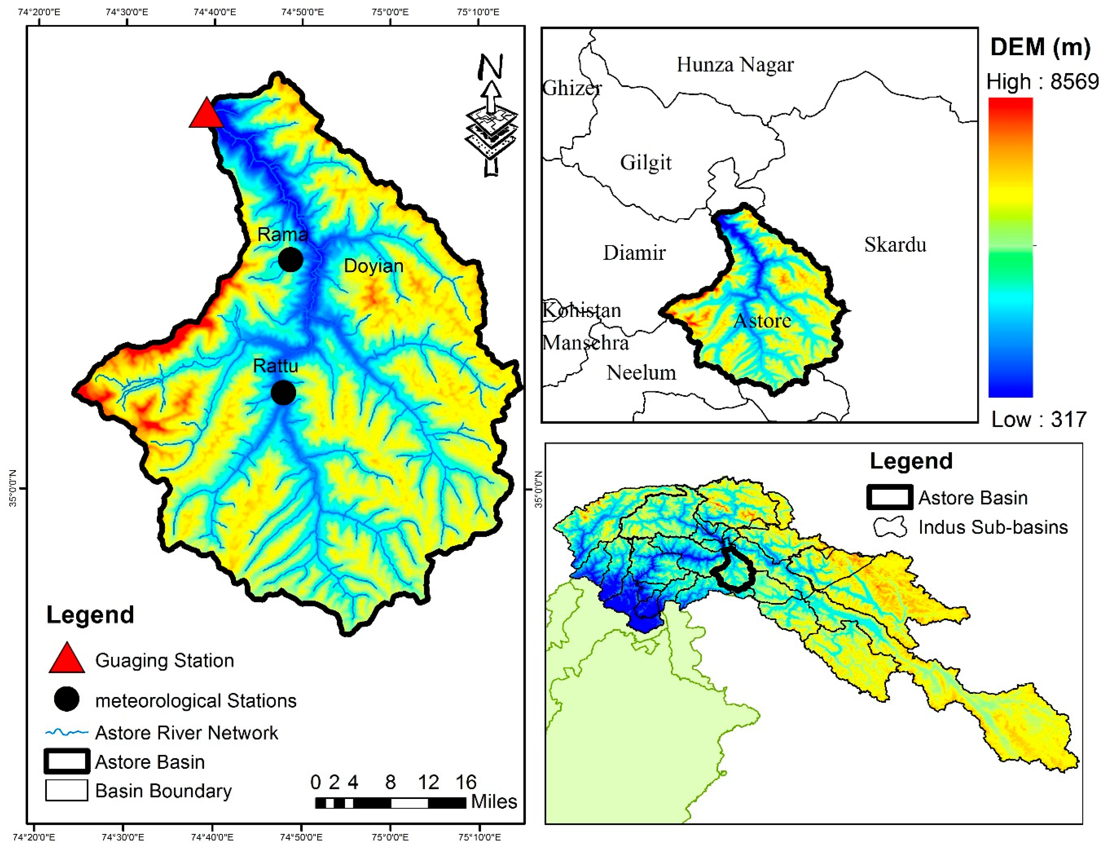
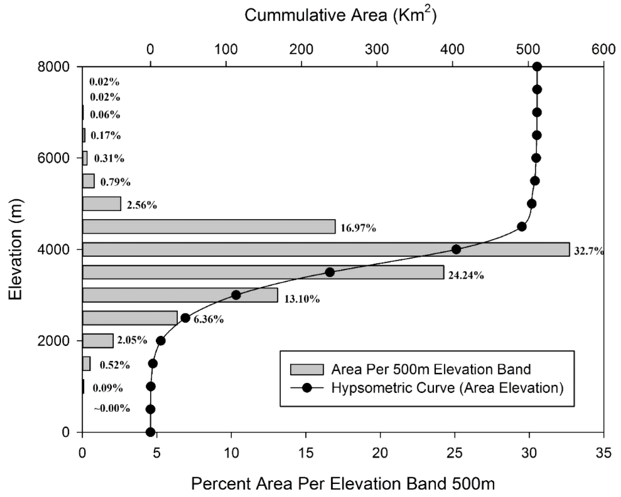
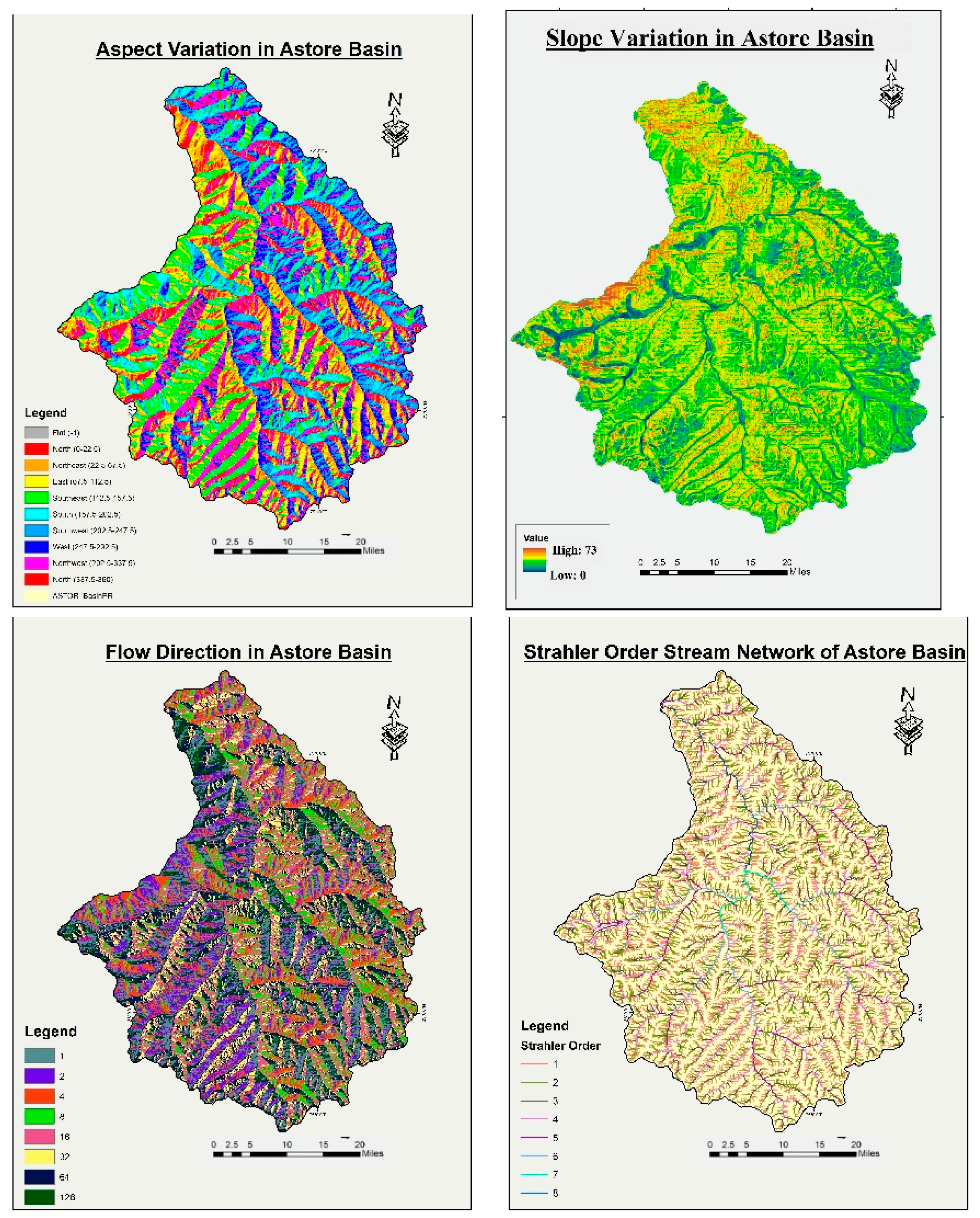
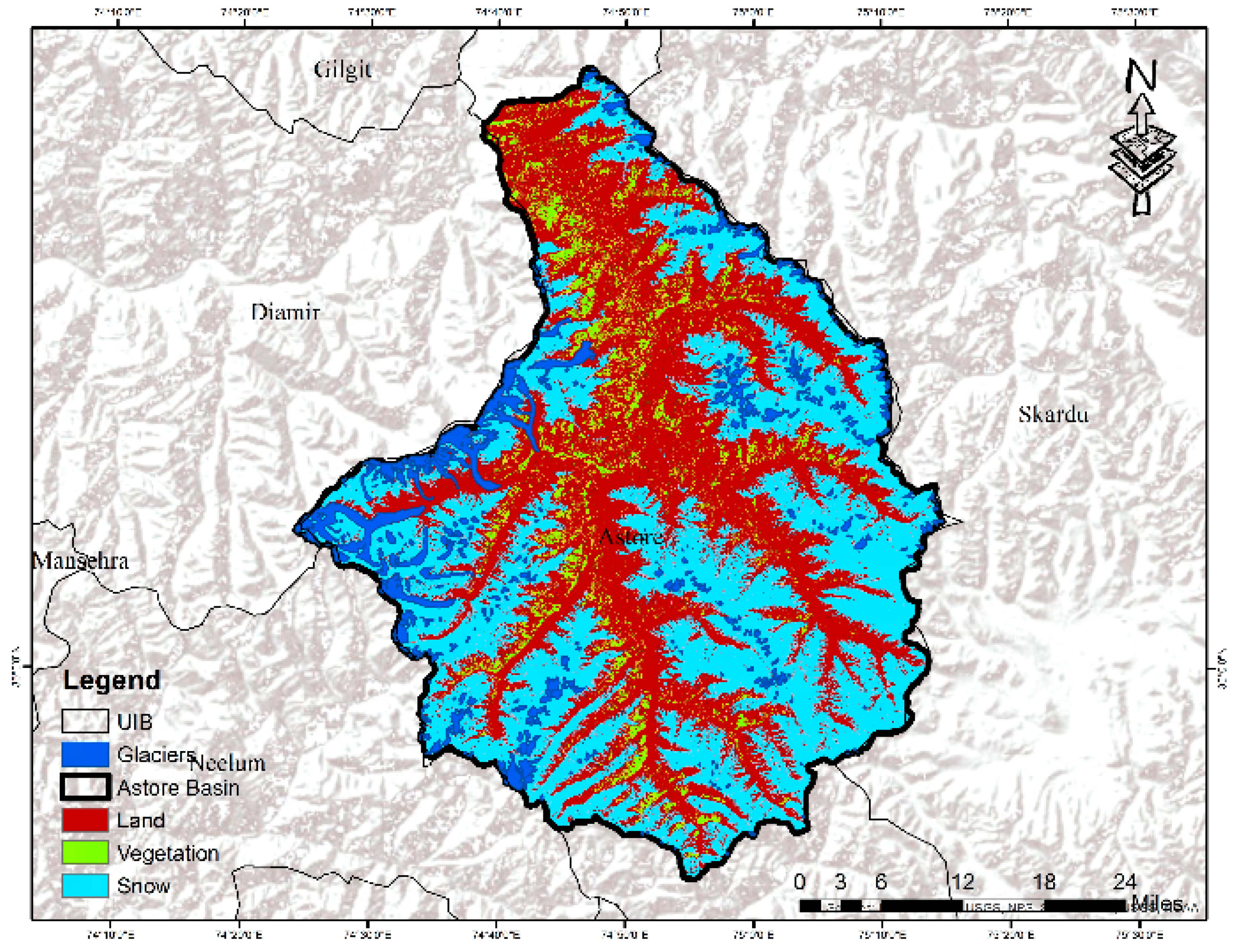
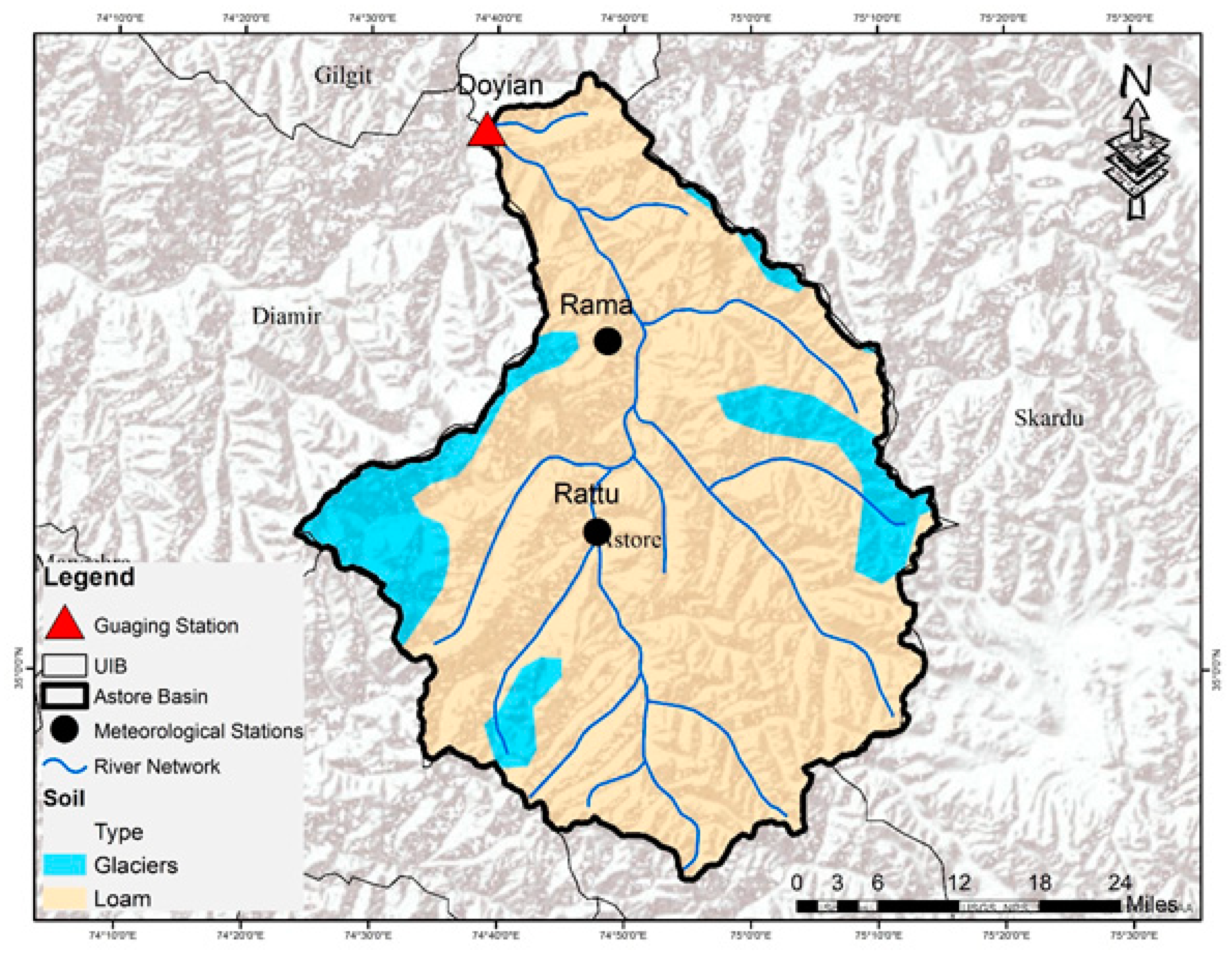
2.1. Study Area

The Astore catchment (a sub-basin of the UIB) located at 35° 33′ N, 74° 42′ E, was selected (Figure 1) for hydro-glaciological modeling under IPCC climate change scenarios. The Astore River basin is located in a northwestern Himalayan arc, with an elevation range 1198 m to 8069 m and total drainage area is about 3988 km2, Figure 2 shows the hypsometric curve. About ~543 km2 area is covered with glaciers with the highest of the peak of Nanga Parbat, which is ranked ninth highest mountain in the world [49]. The average annual temperature during 1998–2012 was 9.9 °C at the station located in valley Rattu (2718 m) and −2.9 °C at the higher altitude Rama station (3179 m).

2.2. TOPKAPI Model

TOPKAPI is a fully distributed physically-based hydrological model that can simulate the high spatial and temporal information on the hydrological state of both small and large watershed [14] and mountainous catchments [50]. The primary inputs required by TOPKAPI model are terrain data or Digital Elevation Models (DEM), soil maps, land cover, glacier boundaries, meteorological data, i.e., temperature and precipitation. Several inputs of soil and hydrological control parameters are required to run the model. Soil parameters includes L (soil depth in m), ks (vertical and horizontal permeability at saturation), ϑr (residual water content), ϑs (saturated water content), αs (non-linear soil exponent of the transmissivity) whereas, routing parameters includes no (manning coefficient for the land cover in m−1/3 s−1) and nc (manning coefficient for the channel in m−1 /3 s−1). Fully distributed physically-based models provide high resolution and more reliable simulations of hydrological behavior towards climate change than empirical or lumped models, which heavily depends on the parameter’s calibration. These models require extensive data input and need to be calibrated and validated to generate all relevant processes accurately [50].
TOPKAPI model has been modified extensively for various application in the mountainous regions to simulate water balance at catchment and sub-catchment scales. The model generates high spatial and temporal outputs for every cell of entire catchment which include time series of hydrologic quantities, i.e., precipitation, air temperature, potential and actual evapotranspiration, snow cover, percolation, surface flow, channel flow, soil moisture and glacier /snow water equivalent. The TOPKAPI model uses the Enhanced Temperature Index (ETI) approach to simulate the glacier and snowmelt component. ETI is an intermediate complexity step between an empirical TIMs and an Energy Balance Models (EBMs) [28,38]. ETI model computes the melt component when the air temperature at specific location of grid cell iTi (°C) exceed the threshold air temperature TT.
Mi= TF.Ti + SRF.IGi * (1 - αi)
where Mi is the melting in a particular cell i (mm water equivalent (w.e.) per day d−1, TF is the temperature factor (mm w.e. K−1 d−1), SRF is the shortwave radiation factor (mm w.e. m2 W−1 d−1), IGi is the incoming shortwave radiation in (Wm−2), and αi is the surface albedo.
The advantage of ETI is that data requirement is not much higher as compared to EBMs. In addition to the air temperature term, the ETI model includes a shortwave radiation term that incorporates incoming solar radiation and albedo that help to account the internal energy of the glacier to provide reliable results. So the TOPKAPI model proved to be more efficient to simulate the glacier melt than the other TIMs and DDMs. With several advantages of TOPKAPI model, it has some limitations that it does not provide the separate output of changes in glacier dynamics and gives the combined hydrograph from glacier melt, snowmelt and precipitation. These output data can be useful to analyze the behavior of the entire basin/sub-basin during severe hydro-meteorological events and can be utilized for preparedness, mitigation, and relief in case of disaster.

2.3. Data Input to Model

The TOPKAPI model input data includes the Digital Elevation Model (DEM) with a spatial resolution of 30 × 30 meters grid, the soil data, the land cover raster, and the hydro-meteorological data (daily average temperature, precipitation, and streamflow).
Figure 3 shows the hydrological and topographical variables derived from the Advanced Spaceborne Thermal Emission and Reflection Radiometer (ASTER) global DEM in the ArcHydro module of Esri’s ArcGIS [43].
Landsat 7 Enhanced Thematic Mapper Plus (ETM+) with a spatial resolution of 30 m was used to generate a Landover map of the Astore basin. Preprocessing (i.e., geometric and atmospheric correction) of Landsat image was done using different filters followed by application of the Maximum Likelihood Classifier (MLC) technique to classify the land cover features that depend on the second-order measurements of a Gaussian probability density function model [51,52]. Figure 4 shows the major land cover classes of Astore basin. TOPKAPI model requires the manning roughness coefficient and crop factor value of all months for each land-use class.
Glacier boundaries were delineated using a morphometric glacier mapping (MGM) technique. The basis in MGM is the use of topographic thresholds derived from a DEM and the multispectral data along with ratio images for the automatic delineation of glacier boundaries. The filters were generated by threshold values defined for the extraction of glaciers. The Normalized Difference Snow Index (NDSI), was used to delineate the glaciers (Figure 4). To further refine the glacier’s boundaries, other filters like Normalized Difference Vegetation Index (NDVI), Land Water Mask (LWM), mean hue [46], slope, and elevation threshold values were used. The delineated glacier outlines were validated using Google Earth’s high-resolution imagery [53].
The FAO global soil dataset [47] with a spatial resolution of 30 arc-second was used to generate the soil data of the Astore basin (Figure 5). The TOPKAPI model requires soil property data such as the soil depth, horizontal and vertical soil hydraulic conductivity, available moisture content, and texture. These soil hydraulic parameters were derived using the PedoTransfer Function (PTF)-based software SoilPAR 2.0 [48] and Soil Water Infiltration and Movement (SWIM) model [49].
Meteorological data of Rama and Rattu stations (1999–2003) comprising of daily average temperature and precipitation and daily flow records (1980 and 2010) at Doiyan gauging station (1583 m asl) of the Astore River was input in the model. This hydro-meteorological dataset was used for model calibration (1999–2000) and validation of model (2001–2003).

Future Climate Projection Data

For future climate change modeling, the Asian Precipitation Highly Resolved Observational Data Integration Toward Evaluation of Water Resources (APHRODITE) dataset was used that has been validated through the actual meteorological stations. The APHRODITE data products V1204R1 and V1101R2 were downloaded for daily temperature and precipitation, respectively. The APHRODITE data was selected to downscale the climate data that can provide the high spatial resolution of 0.1° and 24 h temporal output to fulfill the data input requirement of fully distributed TOPKAPI model. However, APHRODITE data have the limitation that the precipitation measurements are underestimated at a high altitude of UIB, so the bias-corrected APHRODITE temperature and precipitation data were incorporated in the model at a spatial resolution of 0.1°.
In addition to historical data of APHRODITE, Global Climate Models (GCMs) projections generated from the Coupled Model Intercomparison Project Phase 5 (CMIP5) under Representative Concentration Pathways (RCPs) scenarios was also incorporated to assess the climate change impacts on the future hydrology of Astore basin. Four GCMs [54] (i.e., CCSM4, CanESM2, HadGEM2–ES, and GFDL–ESM2M) were selected based on the following criteria (a) models that showed strong correlation (≥ to 0.8) with baseline APHRODITE data (1960–2010), (b) Normalized Root Mean Squared Error (NRMSE) ≤ 0.1 and (c) Normalized Standard Deviations (NSD) was within the range of ±0.4 to that of NSD of APHRODITE time series data.
CCSM4 data with very high correlation (0.94) and less NRMSE value (0.01) was biased corrected under the method of Linear Interpolation and Bias Correction (LIBC) technique [55,56,57]. Linear Interpolation and Bias Correction Method (LIBC) utilizes station data and high-resolution topography, and it is the combination of the geospatial Linear Interpolation (LI) technique in relation with Bias Correction and Spatial Disaggregation (BCSD) technique. BCSD takes account of a correction factor to generate the biased corrected output of GCMs. Bias corrected climate parameters (i.e., temperature and precipitation) of APHRODITE were chosen and interpolated at a resolution of 0.1 degrees for the baseline period 1975–2010. The daily dataset was converted into monthly time series and manipulated to get the climatology and standard deviation of the parameter. A similar process was done for GCMs data, first linearly interpolated at the resolution of APHRODITE, and monthly time series data was manipulated to get the climatology and standard deviation of the parameter. After that correction factors were calculated by the ratio of climatological values of observations to the reference GCMs. Bias corrected APHRODITE datasets have been used in downscaling of baseline GCMs to generate future scenarios daily from the year 2020–2100 with the spatial resolution of 0.1°. This technique eliminates various inaccuracies and the biases related to GCMs data. The result was high resolution gridded projections of temperature and precipitation that used effectively in the TOPKAPI model to predict the hydrological response of the study area at a spatial resolution of 15m grid daily.

2.4. Sensitivity Analysis of the Model Parameters

The sensitivity analysis of various parameters of a hydrological model is assessed to identify which parameter has the highest impact on the model output. The sensitivity of the TOPKAPI model parameters was determined by changing their default values to see each of the parameter’s sensitivity. The initial default values of selected parameters were varied within the upper and lower limits as suggested by literature and documentation of the TOPKAPI model [58,59] as highlighted in Table 1. The model’s sensitivity against these parameters was evaluated by comparing the observed and simulated discharge through Nash efficiency statistics. Based on the visual and statistical agreement between the observed and simulated discharge the most sensitive parameters, affecting the hydrology of the basin were selected [60] for tuning in the calibration process of the TOPKAPI model. In this study, the most sensitive parameters were the depth of surface soil layer (L), saturated hydraulic conductivity (Ks), Residual soil moisture content (θr) and saturated soil moisture content (θr).

Model Calibration and Validation

The TOPKAPI model, like other physically-distributed models, is subjected to several uncertainties associated with the input data. These uncertainties may be due to topographic variation, land cover types, soil properties, approximation methods and tables used to infer physical parameters from the data, and the approximations introduced by the scale of the parameter representations [61]. For these reasons, Liu and Todini [15] suggested that the calibration of parameters is still necessary, but all studies dealing with the TOPKAPI model suggested that the model calibration can be achieved through simple hit and trial method, as we had also done in this current study for Astore basin.
In this current study, an automatic model calibration method i.e., Ordered Physics-based Parameter Adjustment Method (OPPA), as proposed by Vieux, et al. [62] was used for the model calibration. The OPPA is the most effective and time-saving method recommended for the calibration of physically distributed hydrological models, as this method calibrates a model in a specific order [62,63,64]. Initially, the method adjusts the runoff generation parameters to minimize the discharge volume objective function and then those parameters which controlled the runoff routing to minimize the discharge timing objective function. Through the sensitivity analysis and literature Liu, Martina and Todini [14] it was found that soil depth L and soil conductivity Ks are the most sensitive runoff generation factors while the runoff routing is mainly controlled by the Manning roughness of the channel nc and the over-land surface.
Another important parameter, i.e., soil moisture Vs_initial was also tuned because of its high sensitivity towards the runoff generation. To initialize the soil moisture parameter in the model, it was assumed that there was no surface water over the slopes and the water depth in a generic channel cell increases as a linear function of the channel width of the cell. At the beginning of the calibration process, the initial value for soil moisture percentage was set according to dry condition. Then the model was run to find the soil moisture situation at a specific time when the soil should be in the same state as the initial condition. This OPPA method provides accurate and realistic values based on the values for the initial condition, especially concerning the spatial distribution of the saturation percentage. According to Vieux, Cui, and Gaur [62] and others [65,66,67], the hydrological models cannot be calibrated at each pixel level. However, a multiplicative factor can be used for the whole basin. In this study, the four multiplicative factors L (for the soil depth), Ks (for the hydraulic conductivity), no (for the overland roughness) and nc (for the channel roughness) were applied for the model calibration.
The parameters were grouped into (L, Ks, Vs) and (no, nc) because they were independent of each other, i.e., the change in the first group was affecting the quantity and change in second was affecting the timing of runoff at Astore basin (Table 1). Three different statistical measures as recommended through literature, i.e., Index of Agreement (d), R2 and Nash–Sutcliffe Efficiency (NSE) coefficients were used to assess the efficiency of calibration by comparing modeled and observed discharge volumes aggregated on a daily and monthly basis [68,69,70,71].
Before further application of a hydrological model for future forecasting, it is recommended that the validation of the model should be done for a better understanding of spatio–temporal performance of the model. Hence, after the model calibration, validation of TOPKAPI model was done on the remaining hydrological data (2001–2002) to evaluate the performance of simulation and prediction model based on the statistical value of R2, Index of agreement between the simulated and observed discharge and Nash–Sutcliffe Efficiency (NSE) coefficients [75].

3. Results and Discussion

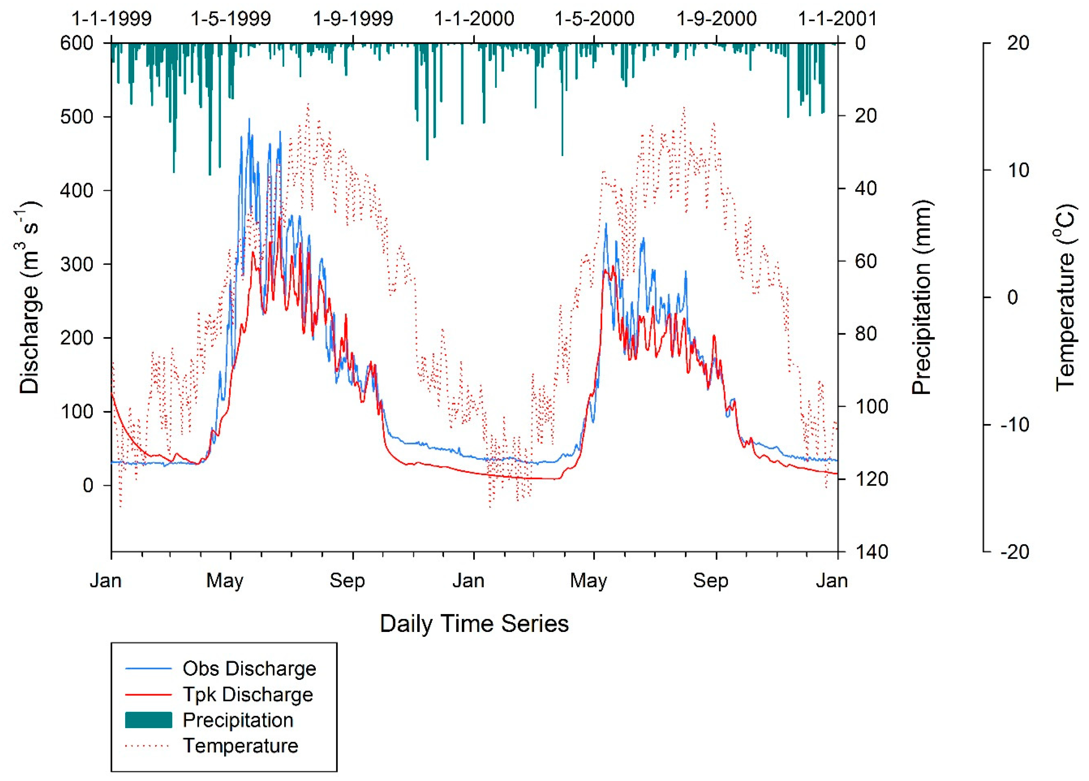
3.1. Model Calibration

The TOPKAPI model calibration (1999–2000) had a significant (p ≤ 0.05) relationship between observed and simulated Astore River discharge with an R2 value of 0.96 and Nash–Sutcliffe efficiency value of 0.95 (Table 2). Figure 6 shows the comparison between the observed and TOPKAPI model simulated discharge along with temperature and precipitation in the basin.
The maximum average flow during the calibration period was observed throughout the summer season (model 188m3.s−1, observed 190 m3.s−1), whereas discharge started increasing in late April and reached its peak in June. This hydrological response of the Astore basin could be due to summer monsoonal liquid precipitation in the basin. Additionally, the higher temperature 12 °C than the average temperature in the basin during the summer season caused increased melting of snow/glaciers resulting in peak discharges of Astore basin. Several research studies also reported a similar trend in hydro-meteorological data [77,78,79]. Whereas, moderate river flow was observed in the late summer (model 81 m3.s−1, observed 85 m3.s−1) with a decrease in discharge started in late August till mid of October. This hydrological pattern of the basin is also in confirmation with temperature trends during a similar period. In winter, the river discharge was very low (model 30 m3.s−1, observed 38 m3.s−1), which shows a close relationship with the temperature of the basin. As the temperature of the basin is at its minimum below 0°C, hence the precipitation in winter is solid, i.e., snowfall. This snowfall caused the accumulation of glaciers and snow in the high altitudes (>4500 m) [52,79,80].

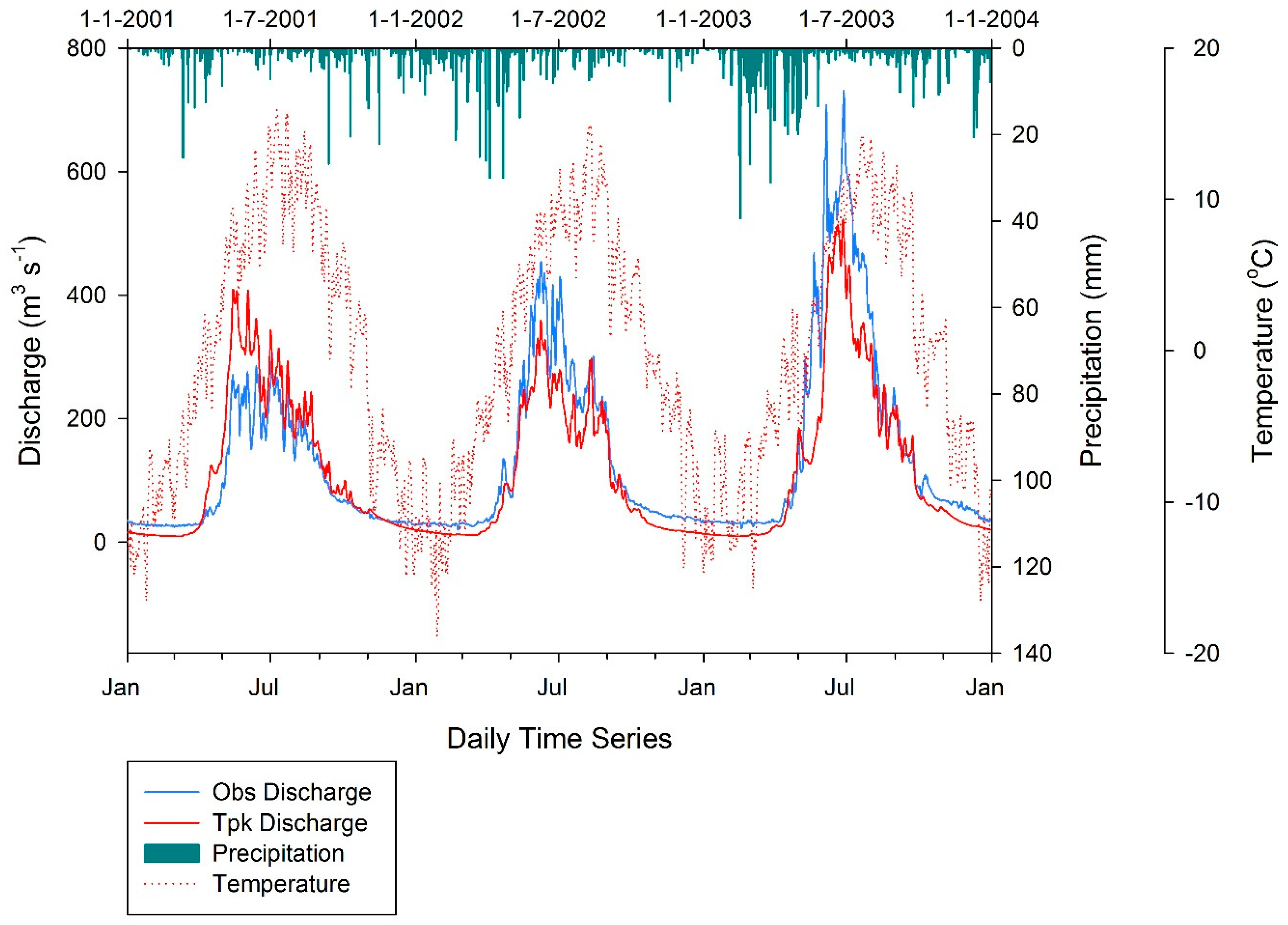
3.2. Model Validation

Figure 7 shows a comparison of simulated and observed discharge at Doiyan (Astore River Basin outlet) along with the trend of the temperature and precipitation, during the validation period 2001–2003. Table 3 depicts the R2, Nash–Sutcliffe efficiency (NSE), and index of agreement (d) statistics. The 2001 validation period had higher R2 and NSE values. However, there was no significant difference.
The maximum average flow during the validation period was observed throughout the summer season (model 199m3.s−1, observed 257m3.s−1, whereas discharge started increasing in late April and reached its peak in June during 2001–2003. This hydrological response of the Astore basin could be because of the monsoonal liquid precipitation in the basin. Additionally, the increase in temperature during the season caused an increased melting of snow/glaciers resulting in the peak discharges. Whereas, moderate river flow was observed in the late summer (model 98 m3.s−1, observed 84 m3.s−1) with a decrease in discharge started in late August till mid of October. This hydrological pattern of the basin is also in resemblance with temperature trend for the same months. In winter, the river discharge was very low (model 28 m3.s−1, observed 39 m3.s−1), which shows a close relationship with the temperature of the basin.
It was observed that about 89.74% of runoff volume generated in the summer season (May–September) due to higher glacier/snow meltwater and summer monsoonal rainfall, whereas insignificant runoff, was observed during winter since most precipitation received as snow in the basin during 1999–2003. Winter runoff was mainly base-flow generated from snowmelt water that was stored in the soil.
Figure 8 shows significant relationships between observed and simulated Astore river daily discharge for the calibration and validation period. The minimum NSE coefficient value never dropped below 0.93 during the entire validation period. The best performance of the model was found over the calibration period with the NSE coefficient value of 0.95, and according to Moriasi, et al. [81], a hydrological model is well calibrated for a runoff if monthly NSE ≥ 0.65. Besides the runoff generation, the TOPKAPI model also generates several other outputs as given in Table 4.
An analysis of snow cover, percolation, evapotranspiration, soil moisture, temperature, snow water equivalent (SWE) and precipitation are vital for understanding the integrated hydrologic response of a catchment. The accurate estimation of basin-wide SWE is the most important unsolved problem in mountain hydrology [82], particularly in the HKH region. The SWE is the amount of water contained within the glacier, which can be taken as the amount of water that would theoretically result if the entire snowpack is being melted instantaneously [83]. TOPKAPI model efficiently simulated the SWE in the Astore river basin, and the results showed that the maximum SWE was found in April (453.86 mm) just after the end of the snow accumulation period, i.e., winter and the lowest value was found in September (11.98 mm) at the end of the summer period. The other significant output of the TOPKAPI model is snow cover extent; the results indicate that the average snow-covered in two seasons, i.e., in winter (November to April) and summer (May to October) was 91 % and 11% respectively. A similar snow cover trend was reported by Atif, Iqbal, and Mahboob [78], they reported that the snow cover in the Astore basin varies from 92% during winter to 15% in summer seasons.

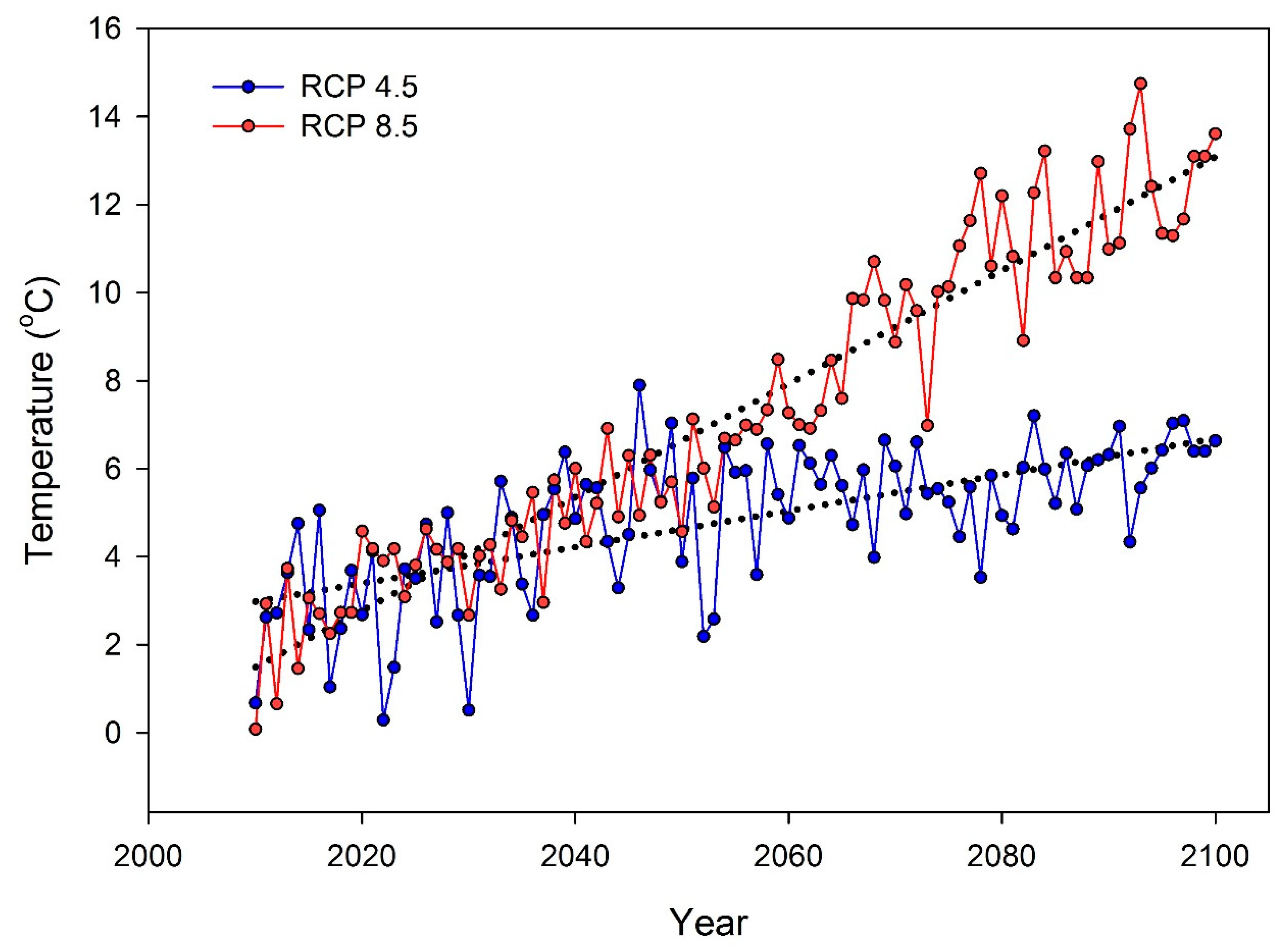
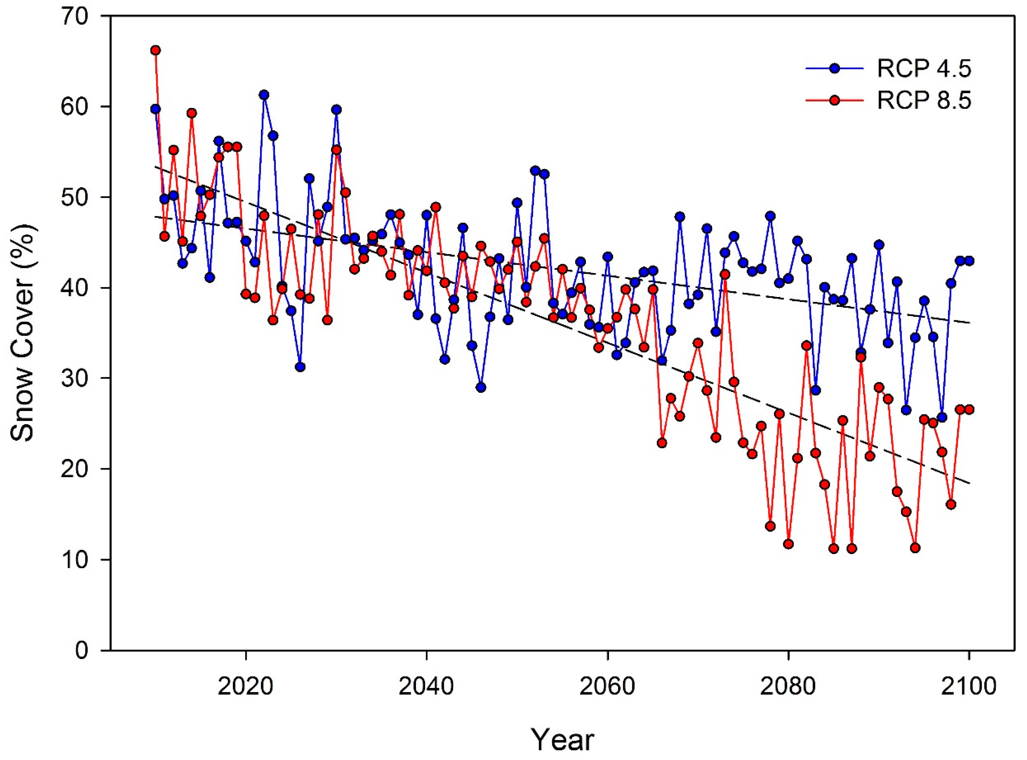
3.3. Future Climate Projections (2010–2100)

Very fine resolution future climatic data (temperature and precipitation) acquired by the CMIP5 model were downscaled under the two Representative Concentration Pathways scenarios (RCP4.5 and RCP8.5) and used to forecast the future hydrology of Astore. Monthly climate change for the three periods (2010–2040, 2041–2070, and 2071– 2100) is summarized in Table 5 and Table 6.
Towards the end of this century, an increase of 0.03 °C and 0.12 °C in annual temperature was observed under RCP4.5 and RCP8.5, respectively. The analysis showed that under RCPs the summer temperatures would be high as compared to the base data, i.e., 3.4 °C high in RCP4.5 and 6.4 °C in RCP8.5 (Figure 9). Research studies conducted by Kazmi has also supported our results. Rajbhandari, et al. [84] and Ul Islam, et al. [85], which concluded an increase in future temperature by 4.8 °C at the end of this century using PRECIS Regional Climate Model (RCM) model.
Under the RCP8.5 and RCP4.5 mean precipitation projection shows an increasing trend. Generally, the RCP8.5 scenario shows an 11% significant (p ≤ 0.05) increase at the end of this century. Several studies reported a similar increasing trend in precipitation in the UIB, for example, Beven [13] reported a 25% precipitation increase compared to the baseline period (2046–2065) based on the results of five General Circulation Models (GCMs). Also, Rajbhandari, Shrestha, Kulkarni, Patwardhan, and Bajracharya [84] forecasted an increase in precipitation up to 21% using the PRECIS fine-resolution RCM. Another study conducted by Forsythe, et al. [86] also reported an increase of precipitation in the UIB by applying a stochastic rainfall model. All of the above studies projected an increasing trend in the UIB precipitation regardless of using different methodologies to conclude. However, uncertainties exist in the magnitude of precipitation projected by these studies. Since we also found similar uncertainties regarding our precipitation projections, therefore it is important to conduct further studies at the basin level to reduce those uncertainties.

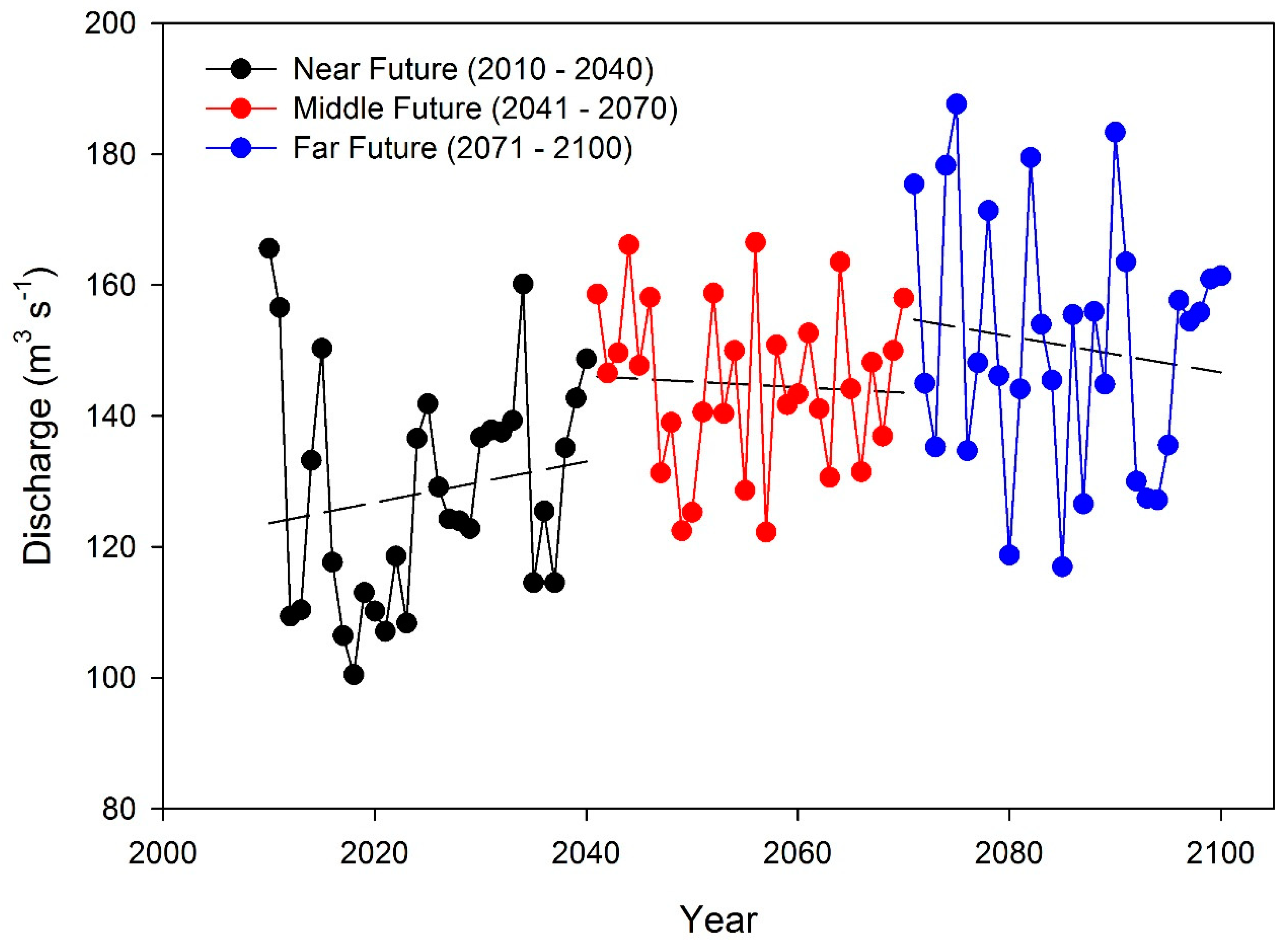
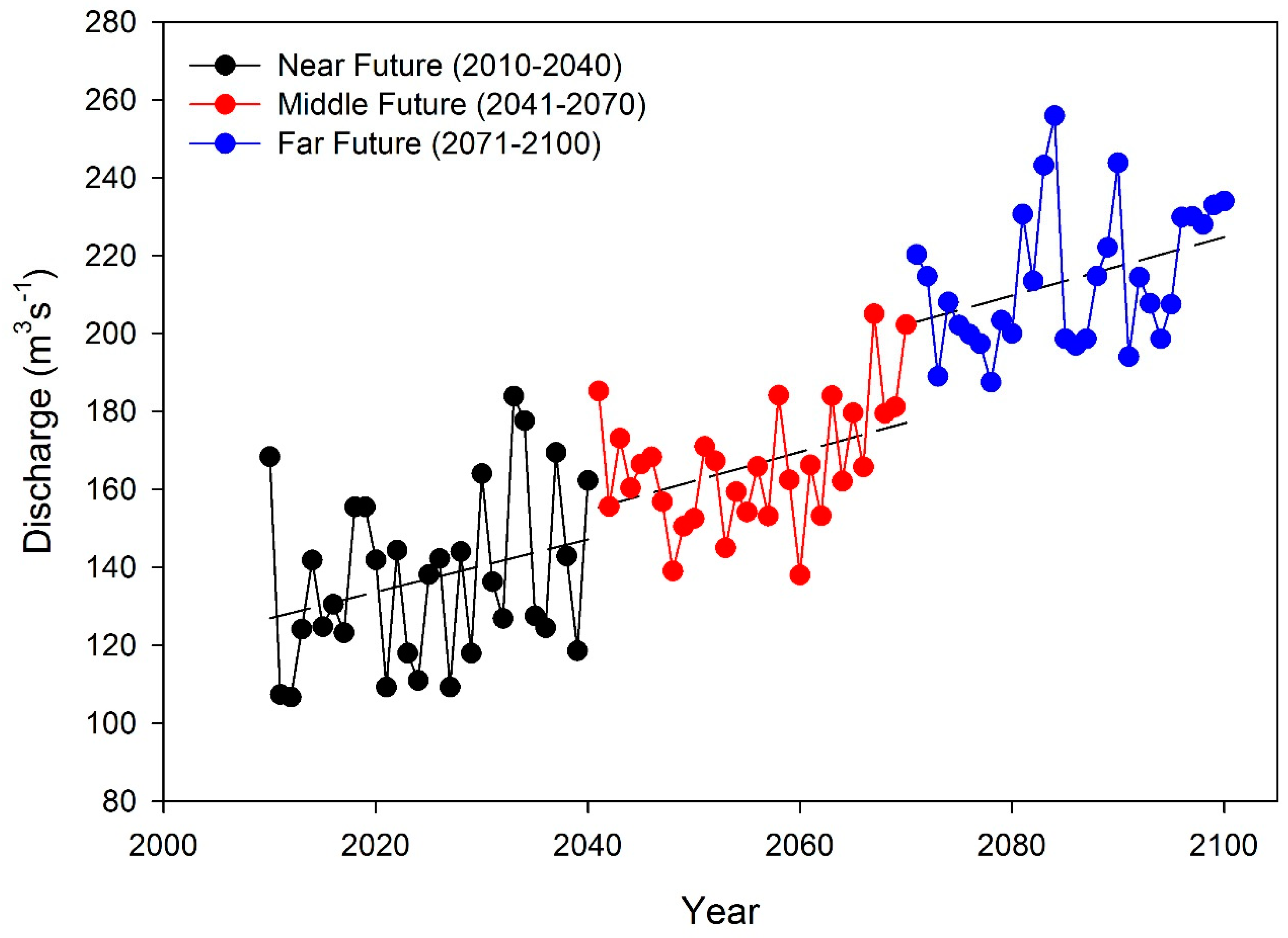
3.4. Future (2010–2100) Hydrological Flows Trend

The TOPKAPI model simulated a negative snow cover projections trend of −0.12%.yr−1 and −0.39%.yr−1 under IPCC climate scenarios RCPs 4.5 and 8.5, respectively during 2010–2100 (Figure 10). The corresponding decrease in snow cover ranged from 47% to 35% and 55% to 21% for RCP4.5 and RCP8.5 scenarios, respectively during the end of this century 2100. The mean snow cover area was 46% during the near future (2010–2040); 38% during the middle future (2041–2070) and 22% during far future projection (2071–2100) under RCP8.5. Whereas under RCP4.5, mean snow cover area was found to be 47% during (2010–2040); 39% during the middle future (2041–2070) and snow cover extent remained the same during (2071–2100).
Figure 11 shows an increasing trend in the monthly projected discharge of River Astore under different climatic scenarios. Under the RCP8.5 scenario the discharge increased significantly (p ≤ 0.05) from 196 m3.s−1 to 220 m3.s−1, whereas a non-significant increase in river discharge was observed starting from 124 m3.s−1 with the maximum value of 151 m3.s−1 under RCP4.5 towards the end of the century.
Mean annual discharge increased by 127.65 m3.s−1 to 136 m3.s−1 during near future scenario (2010–2040); whereas the decreasing trend was observed during the middle future (2041–2070) from 150 m3.s−1 to 145.8 m3.s−1 and the discharge situation remained same at the end of 21st century under RCP4.5. Whereas under RCP8.5, mean annual discharge increased by 125 m3.s−1 to 150 m3.s−1 during (2010–2040); 160 m3.s−1 to 180 m3.s−1 during middle future (2041–2070) and 210 m3.s−1 to 230 m3.s−1 during far future (2071–2100) projection (Figure 12 and Figure 13).

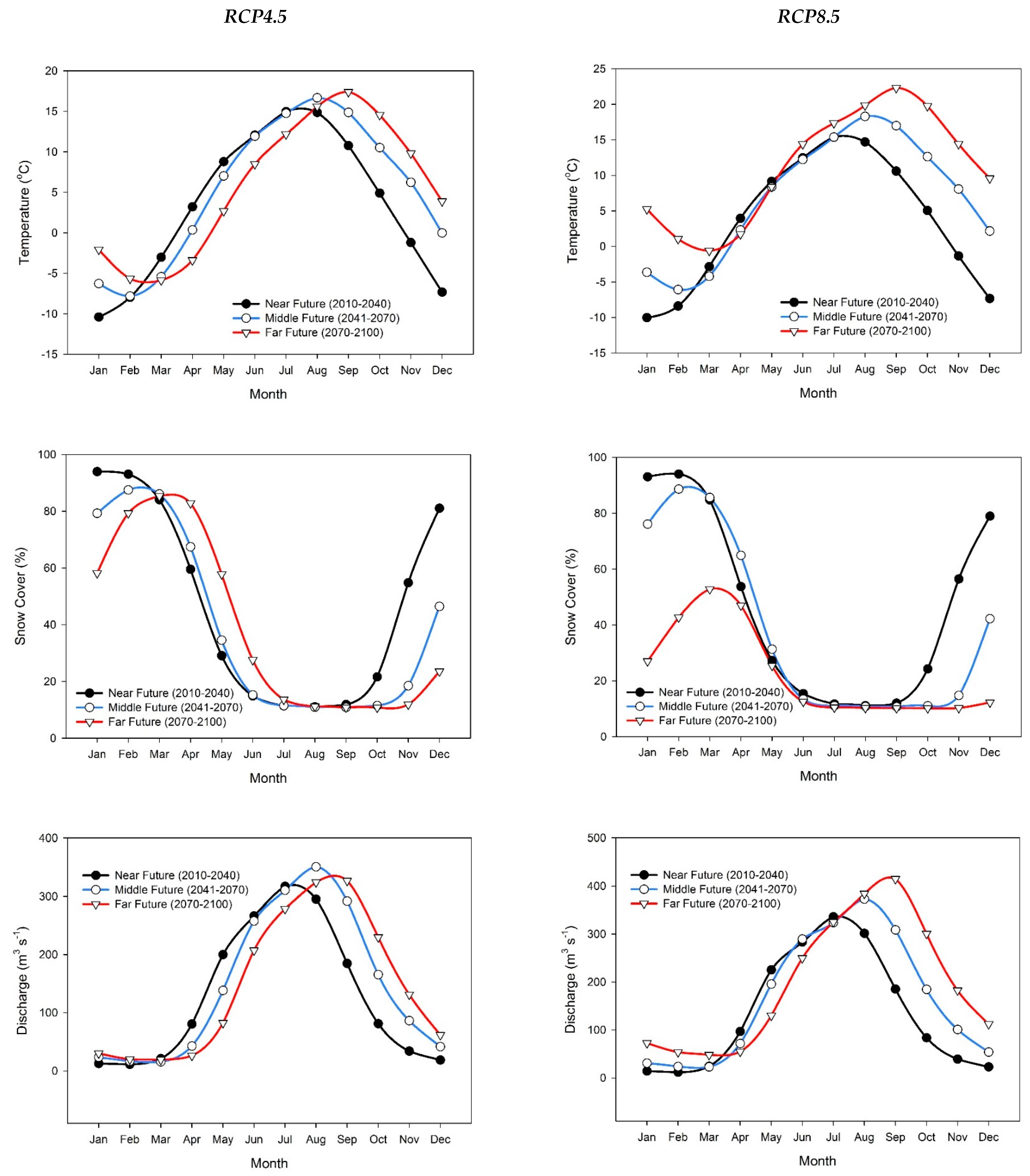
3.5. Pattern of Hydroclimatic Shift in Astore Basin

Throughout the world, the pattern of the hydroclimatic shift has been reported by many [87,88]. However, its magnitude varies spatially on a regional scale. Temporal changes in streamflow in the Astore basin shows a pattern of seasonal shifts showing a substantial decrease in flow during March–July (Figure 14). On the other hand, it shows a slight increase in discharge during autumn and winter seasons. Historically the Astore basin had a large rainfall-runoff and snowmelt components; however, the reduction in precipitation during spring and the monsoon along with an increase in evapotranspiration will most likely cause a decrease in runoff (Figure 14). The mean projection for RCP8.5 for the period 2071–2100 also shows the same intra-annual pattern for the near future but with more intensity. Many studies [5,84,85] has projected the receding of the glaciated areas in the UIB, which will significantly reduce the share of glacial meltwater that will ultimately cause a reduction in the discharge during the summer season. Also, the decline in the glacier meltwater, our analysis shows a reduction in the monsoon precipitation along with a highly significant (p ≥ 0.01) increase in evapotranspiration in the RCP4.5 and RCP8.5 climate change scenarios. The earlier onset of snow and glacier melt will cause more increase in Astore river flow as indicated by discharge results. This change in hydrological pattern might have strong implication for the cropping pattern and onset of the sowing seasons for different crops in the downstream agricultural areas, especially for Punjab known as the breadbasket of Pakistan.
The results of future forecasted flows are in line with studies conducted by another researcher in sub-basins of UIB [86]. Initially, the summer river runoff will be increased by the mid 21st century and will ultimately decrease at the end of the 21st century. Whereas, for the spring season it will be increased throughout the years. Overall the Astore river flow will be increased, and it is in accordance with the flow of UIB as reported by [87]. These studies used the same RCP 4.5 and RCP 85 scenarios for future forecasting of the hydrology of UIB. However, the comparisons of the results of this study with the results of other studies are subject to the use of different climate models and future scenarios. The uncertainties in hydrological forecasting have also been reported by Prudhomme, et al. [88] at UIB level.
Uncertainties in climate and hydrology projections exist due to the scale of application, data quality and scarcity lead to use of same parameter data for entire complex topography, model forcing etc. The uncertainties exist in the parameterization of modeling are challenging. However, the emphasis should be given to the uncertainties in input data and how they simulate the hydrology of basin. Several scientists [8,76,89,90,91] reported that the rain gauge at high altitude could capture only 20%–30% of precipitation due to topographical variation, blowing and drifting of snow, high-pressure wind. Jonas et al., 2009 reported the range of uncertainty is 13% and 30% in observational data Gigerwald valley. To minimize the uncertainty in observational data Zweifel and Sevruk [92] suggested that wind and evapotranspiration data should be considered for the correction of precipitation. Another factor of uncertainty is that the basin-wide extrapolation of precipitation from the scarce gauges will generate an inappropriate outcome and also the correction of precipitation in high glacierized regions may not be possible due to high altitudinal variation and its dependency on climate forcing [93]. So for an accurate assessment of water resources there is a dire need to have high-quality observational data from dense meteorological stations. The uncertainty of hydrological model does not only depend on the observational data but also on the evaluation criteria of model calibration. In this study model calibration was assessed by three evaluation methods d, R2 and NSE coefficients that showed the significantly good agreement with the observed data.
For the downscaling and correction of Global Climate Models GCMs the reference APHRODITE data was used. The gridded APHRODITE data also introduced uncertainty because the data was biased corrected based on a lack of knowledge of glacier mass balance [94]. Finger et al., 2012 stated the glacier and snow dominant catchments and downscaling method of GCMs introduce the significant uncertainty in projected climate change scenario. The uncertainty in climate projection and statistical downscaling method LIBC was evaluated using the QUMP (Quantifying Uncertainty in Model Prediction) ensemble data [95].Temperature lapse rate and precipitation gradient factors for statistical downscaling of RCP4.5 and RCP8.5 reduced the uncertainty in resolving the complex topography of Astore basin. The LIBC technique minimizes the error from a range of 1.7–11.3 °C to a range of 1.4–4.0 °C and negative slopes of linear regression model depicted that error has reduced in the projected downscaled data of temperature as compared to raw GCM data.

4. Conclusions

The present study is the first application of the fully distributed hydrological TOPKAPI model in the Astore catchment, which was focused on the climate projection under RCP4.5 and 8.5 to assess the impact on the hydrological regime of UIB. The TOPKAPI model was successfully calibrated and validated in the Astore river basin using an advance Ordered Physics-based Parameter Adjustment Method OPPA. From the results and statistical measures, it can be concluded that the TOPKAPI model performed efficiently for both the calibration and validation periods. The future forecasting of the hydrology of Astore basin showed a non-significant increase in summer flows and an increased flow during other seasons from 2021 to 2050. Whereas from 2071 to 2100 the summer flows were also found to be decreased with a sharp increase in flows during the other seasons. Overall the increasing trend in Astore river discharge and decreasing trend in snow cover was observed, which can be related to the increase in precipitation (rainfall), temperature and evapotranspiration. The results of this study should, therefore, consider and incorporate into water resources management plans and development of water policy for future water storage in proposed Diamer-Basha Dam and other planned reservoirs on the Indus River system.

Author Contributions

I.A. and J.I. conceived and designed the study; I.A. run the TOPKAPI model and collected and analyzed all the data. I.A. wrote the first draft of the paper, J.I. extensively reviewed the article. L.-j.S. reviewed the paper and suggested valuable inputs also provided partial funding for research.

Funding

The work presented here is part of a Ph.D. research study and was supported by the National University of Sciences and Technology (NUST), Islamabad, Pakistan, using the student research fund.

Acknowledgments

The Authors acknowledge the Pakistan Water and Power Development Authority (WAPDA) for providing the ground-based meteorological data. We appreciate and thank NASA’s Earth Science Data Systems Program the “Earth Observing System Data and Information System” for managing and providing the satellite data products freely to the public. The author also acknowledges the unanimous reviewers for their review and valuable inputs.

Conflicts of Interest

The authors declare no conflict of interest.

References

  1. Bolch, T.; Kulkarni, A.; Kääb, A.; Huggel, C.; Paul, F.; Cogley, J.; Frey, H.; Kargel, J.S.; Fujita, K.; Scheel, M. The state and fate of Himalayan glaciers. Science 2012, 336, 310–314. [Google Scholar] [CrossRef] [PubMed]
  2. Kapnick, S.B.; Delworth, T.L.; Ashfaq, M.; Malyshev, S.; Milly, P.C. Snowfall less sensitive to warming in Karakoram than in Himalayas due to a unique seasonal cycle. Nat. Geosci. 2014, 7, 834. [Google Scholar] [CrossRef]
  3. Cannon, F.; Carvalho, L.M.; Jones, C.; Bookhagen, B. Multi-annual variations in winter westerly disturbance activity affecting the Himalaya. Clim. Dyn. 2015, 44, 441–455. [Google Scholar] [CrossRef]
  4. Berghuijs, W.; Woods, R.; Hrachowitz, M. A precipitation shift from snow towards rain leads to a decrease in streamflow. Nat. Clim. Chang. 2014, 4, 583. [Google Scholar] [CrossRef]
  5. Adnan, M.; Nabi, G.; Poomee, M.S.; Ashraf, A. Snowmelt runoff prediction under changing climate in the Himalayan cryosphere: A case of Gilgit River Basin. Geosci. Front. 2017, 8, 941–949. [Google Scholar] [CrossRef] [Green Version]
  6. Ahmed, M. Democracy and Corruption. 2018. Available online: https://dailytimes.com.pk/246272/democracy-and-corruption/ (accessed on 11 July 2018).
  7. Tahir, A.A.; Chevallier, P.; Arnaud, Y.; Neppel, L.; Ahmad, B. Modeling snowmelt-runoff under climate scenarios in the Hunza River basin, Karakoram Range, Northern Pakistan. J. Hydrol. 2011, 409, 104–117. [Google Scholar] [CrossRef]
  8. Akhtar, M.; Ahmad, N.; Booij, M.J. The impact of climate change on the water resources of Hindukush–Karakorum–Himalaya region under different glacier coverage scenarios. J. Hydrol. 2008, 355, 148–163. [Google Scholar] [CrossRef]
  9. Bookhagen, B.; Burbank, D.W. Toward a complete Himalayan hydrological budget: Spatiotemporal distribution of snowmelt and rainfall and their impact on river discharge. J. Geophys. Res. Earth Surf. 2010, 115, F3. [Google Scholar] [CrossRef]
  10. Mahmood, R.; Jia, S.; Babel, M.S. Potential impacts of climate change on water resources in the Kunhar River Basin, Pakistan. Water 2016, 8, 23. [Google Scholar] [CrossRef]
  11. Gudmundsson, L.; Wagener, T.; Tallaksen, L.; Engeland, K. Evaluation of nine large-scale hydrological models with respect to the seasonal runoff climatology in Europe. Water Resour. Res. 2012, 48. [Google Scholar] [CrossRef]
  12. Rees, H.G.; Collins, D.N. Regional differences in response of flow in glacier-fed Himalayan rivers to climatic warming. Hydrol. Process. Int. J. 2006, 20, 2157–2169. [Google Scholar] [CrossRef]
  13. Beven, K.J. Uniqueness of place and process representations in hydrological modelling. Hydrol. Earth Syst. Sci. Discuss. 2000, 4, 203–213. [Google Scholar] [CrossRef] [Green Version]
  14. Liu, Z.; Martina, M.L.; Todini, E. Flood forecasting using a fully distributed model: Application of the TOPKAPI model to the Upper Xixian Catchment. Hydrol. Earth Syst. Sci. Discuss. 2005, 9, 347–364. [Google Scholar] [CrossRef]
  15. Liu, Z.; Todini, E. Towards a comprehensive physically-based rainfall-runoff model. Hydrol. Earth Syst. Sci. Discuss. 2002, 6, 859–881. [Google Scholar] [CrossRef]
  16. Kampf, S.K.; Burges, S.J. A framework for classifying and comparing distributed hillslope and catchment hydrologic models. Water Resour. Res. 2007, 43. [Google Scholar] [CrossRef] [Green Version]
  17. Duan, Q.; Sorooshian, S.; Gupta, V. Effective and efficient global optimization for conceptual rainfall-runoff models. Water Resour. Res. 1992, 28, 1015–1031. [Google Scholar] [CrossRef]
  18. Cruz, R.; Harasawa, H.; Lal, M.; Wu, S.; Anokhin, Y.; Punsalmaa, B.; Honda, Y.; Jafari, M.; Li, C.; Huu Ninh, N. Asia. In Climate Change 2007: Impacts, Adaptation and Vulnerability—Contribution of Working Group II to the Fourth Assessment Report of the Intergovernmental Panel on Climate Change; Parry, M.L., Canziani, O.F., Palutikof, J.P., van der Linden, P.J., Hanson, C.E., Eds.; Cambridge University Press: Cambridge, UK, 2007; pp. 469–506. [Google Scholar]
  19. Immerzeel, W.W.; Droogers, P.; De Jong, S.; Bierkens, M. Large-scale monitoring of snow cover and runoff simulation in Himalayan river basins using remote sensing. Remote Sens. Environ. 2009, 113, 40–49. [Google Scholar] [CrossRef]
  20. Beniston, M. Climatic change in mountain regions: A review of possible impacts. In Climate Variability and Change in High Elevation Regions: Past, Present & Future; Springer: Berlin, Germany, 2003; pp. 5–31. [Google Scholar]
  21. Zhang, L.; Su, F.; Yang, D.; Hao, Z.; Tong, K. Discharge regime and simulation for the upstream of major rivers over Tibetan Plateau. J. Geophys. Res. Atmos. 2013, 118, 8500–8518. [Google Scholar] [CrossRef]
  22. Zhao, Q.; Zhang, S.; Ding, Y.J.; Wang, J.; Han, H.; Xu, J.; Zhao, C.; Guo, W.; Shangguan, D. Modeling hydrologic response to climate change and shrinking glaciers in the highly glacierized Kunma Like River Catchment, Central Tian Shan. J. Hydrometeorol. 2015, 16, 2383–2402. [Google Scholar] [CrossRef]
  23. Ren, Z.; Su, F.; Xu, B.; Xie, Y.; Kan, B. A Coupled Glacier-Hydrology Model and Its Application in Eastern Pamir. J. Geophys. Res. Atmos. 2018, 123, 13692–13713. [Google Scholar] [CrossRef]
  24. Archer, D. Contrasting hydrological regimes in the upper Indus Basin. J. Hydrol. 2003, 274, 198–210. [Google Scholar] [CrossRef]
  25. Fowler, H.; Archer, D. Conflicting signals of climatic change in the Upper Indus Basin. J. Clim. 2006, 19, 4276–4293. [Google Scholar] [CrossRef]
  26. Singh, P.; Bengtsson, L. Hydrological sensitivity of a large Himalayan basin to climate change. Hydrol. Process. 2004, 18, 2363–2385. [Google Scholar] [CrossRef]
  27. Arnold, N.; Richards, K.; Willis, I.; Sharp, M. Initial results from a distributed, physically based model of glacier hydrology. Hydrol. Process. 1998, 12, 191–219. [Google Scholar] [CrossRef]
  28. Hock, R. Glacier melt: A review of processes and their modelling. Prog. Phys. Geogr. 2005, 29, 362–391. [Google Scholar] [CrossRef]
  29. Devia, G.K.; Ganasri, B.; Dwarakish, G. A review on hydrological models. Aquat. Procedia 2015, 4, 1001–1007. [Google Scholar] [CrossRef]
  30. Freeze, R.A.; Harlan, R. Blueprint for a physically-based, digitally-simulated hydrologic response model. J. Hydrol. 1969, 9, 237–258. [Google Scholar] [CrossRef]
  31. Paparrizos, S.; Maris, F. Hydrological simulation of Sperchios River basin in Central Greece using the MIKE SHE model and geographic information systems. Appl. Water Sci. 2017, 7, 591–599. [Google Scholar] [CrossRef]
  32. Bao, H.; Wang, L.; Zhang, K.; Li, Z. Application of a developed distributed hydrological model based on the mixed runoff generation model and 2D kinematic wave flow routing model for better flood forecasting. Atmos. Sci. Lett. 2017, 18, 284–293. [Google Scholar] [CrossRef] [Green Version]
  33. Kan, G.; Tang, G.; Yang, Y.; Hong, Y.; Li, J.; Ding, L.; He, X.; Liang, K.; He, L.; Li, Z. An improved coupled routing and excess storage (crest) distributed hydrological model and its verification in Ganjiang River Basin, China. Water 2017, 9, 904. [Google Scholar] [CrossRef]
  34. Ciarapica, L.; Todini, E. TOPKAPI: A model for the representation of the rainfall-runoff process at different scales. Hydrol. Process. 2002, 16, 207–229. [Google Scholar] [CrossRef]
  35. Ragettli, S.; Pellicciotti, F.; Immerzeel, W.W.; Miles, E.S.; Petersen, L.; Heynen, M.; Shea, J.M.; Stumm, D.; Joshi, S.; Shrestha, A. Unraveling the hydrology of a Himalayan catchment through integration of high resolution in situ data and remote sensing with an advanced simulation model. Adv. Water Resour. 2015, 78, 94–111. [Google Scholar] [CrossRef]
  36. Ortiz, E.; Guna, V. Distributed hydrological models: Comparison between TOPKAPI, a physically based model and TETIS, a conceptually based model. In Proceedings of the EGU General Assembly 2009, Vienna, Austria, 19–24 April 2009. [Google Scholar]
  37. Shrestha, M.; Koike, T.; Hirabayashi, Y.; Xue, Y.; Wang, L.; Rasul, G.; Ahmad, G.R.A. Integrated simulation of snow and glacier melt in water and energy balance-based, distributed hydrological modeling framework at Hunza River Basin of Pakistan Karakoram region. JGR 2015, 120, 4889–4919. [Google Scholar] [CrossRef] [Green Version]
  38. Pellicciotti, F.; Brock, B.; Strasser, U.; Burlando, P.; Funk, M.; Corripio, J. An enhanced temperature-index glacier melt model including the shortwave radiation balance: Development and testing for Haut Glacier d’Arolla, Switzerland. J. Glaciol. 2005, 51, 573–587. [Google Scholar] [CrossRef]
  39. Pellicciotti, F.; Buergi, C.; Immerzeel, W.W.; Konz, M.; Shrestha, A.B. Challenges and uncertainties in hydrological modeling of remote Hindu Kush–Karakoram–Himalayan (HKH) basins: Suggestions for calibration strategies. Mt. Res. Dev. 2012, 32, 39–50. [Google Scholar] [CrossRef]
  40. Cogley, J.; Hock, R.; Rasmussen, L.; Arendt, A.; Bauder, A.; Braithwaite, R.; Jansson, P.; Kaser, G.; Möller, M.; Nicholson, L. Glossary of glacier mass balance and related terms. IHP-VII Tech. Doc. Hydrol. 2011, 86, 965. [Google Scholar]
  41. Kargel, J.S.; Cogley, J.G.; Leonard, G.J.; Haritashya, U.; Byers, A. Himalayan glaciers: The big picture is a montage. Proc. Natl. Acad. Sci. USA 2011, 108, 14709–14710. [Google Scholar] [CrossRef] [Green Version]
  42. Rango, A. Application of remote sensing methods to hydrology and water resources. Hydrol. Sci. J. 1994, 39, 309–320. [Google Scholar] [CrossRef] [Green Version]
  43. Li, Z.-L.; Tang, R.; Wan, Z.; Bi, Y.; Zhou, C.; Tang, B.; Yan, G.; Zhang, X. A review of current methodologies for regional evapotranspiration estimation from remotely sensed data. Sensors 2009, 9, 3801–3853. [Google Scholar] [CrossRef]
  44. Tang, Q.; Gao, H.; Lu, H.; Lettenmaier, D.P. Remote sensing: Hydrology. Prog. Phys. Geogr. 2009, 33, 490–509. [Google Scholar] [CrossRef]
  45. Wang, L.; Qu, J.J. Satellite remote sensing applications for surface soil moisture monitoring: A review. Front. Earth Sci. China 2009, 3, 237–247. [Google Scholar] [CrossRef]
  46. Zheng, G.; Moskal, L.M. Retrieving leaf area index (LAI) using remote sensing: Theories, methods and sensors. Sensors 2009, 9, 2719–2745. [Google Scholar] [CrossRef] [PubMed]
  47. Dietz, A.J.; Kuenzer, C.; Gessner, U.; Dech, S. Remote sensing of snow—A review of available methods. Int. J. Remote Sens. 2012, 33, 4094–4134. [Google Scholar] [CrossRef]
  48. Skoulikaris, C.; Filali-Meknassi, Y.; Aureli, A.; Amani, A.; Jiménez-Cisneros, B.E. Information-Communication Technologies as an Integrated Water Resources Management (IWRM) Tool for Sustainable Development. Achiev. Chall. Integr. River Basin Manag. 2018, 179–181. [Google Scholar]
  49. Afshan, N.; Khalid, A.; Iqbal, S.; Niazi, A.; Sultan, A. Puccinia subepidermalis sp. nov. and new records of rust fungi from Fairy Meadows, Northern Pakistan. Mycotaxon 2009, 110, 173–182. [Google Scholar] [CrossRef]
  50. Finger, D.; Pellicciotti, F.; Konz, M.; Rimkus, S.; Burlando, P. The value of glacier mass balance, satellite snow cover images, and hourly discharge for improving the performance of a physically based distributed hydrological model. Water Resour. Res. 2011, 47. [Google Scholar] [CrossRef]
  51. Todini, E. The ARNO rainfall—Runoff model. J. Hydrol. 1996, 175, 339–382. [Google Scholar] [CrossRef]
  52. Atif, I.; Mahboob, M.A.; Iqbal, J. Snow cover area change assessment in 2003 and 2013 using MODIS data of the Upper Indus Basin, Pakistan. J. Himal. Earth Sci. 2015, 48. [Google Scholar]
  53. Atif, I.; Iqbal, J.; Mahboob, M.A. Modelling semi-automated delineation of supra-glacial debris and clean ice glacial changes of shigar basin. Geosciences 2016, 9, 259. [Google Scholar]
  54. Farjad, B.; Gupta, A.; Sartipizadeh, H.; Cannon, A. A novel approach for selecting extreme climate change scenarios for climate change impact studies. Sci. Total Environ. 2019, 678, 476–485. [Google Scholar] [CrossRef]
  55. Lazoglou, G.; Anagnostopoulou, C.; Skoulikaris, C.; Tolika, K. Bias Correction of Climate Model’s Precipitation Using the Copula Method and Its Application in River Basin Simulation. Water 2019, 11, 600. [Google Scholar] [CrossRef]
  56. Wood, A.W.; Leung, L.R.; Sridhar, V.; Lettenmaier, D. Hydrologic implications of dynamical and statistical approaches to downscaling climate model outputs. Clim. Chang. 2004, 62, 189–216. [Google Scholar] [CrossRef]
  57. Immerzeel, W.W.; Van Beek, L.; Konz, M.; Shrestha, A.; Bierkens, M. Hydrological response to climate change in a glacierized catchment in the Himalayas. Clim. Chang. 2012, 110, 721–736. [Google Scholar] [CrossRef] [PubMed]
  58. Ross, P.J. SWIM: A Simulation Model for Soil Water Infiltration and Movement: Reference Manual; CSIRO: Canberra, Australia, 1990. [Google Scholar]
  59. Coccia, G.; Mazzetti, C.; Ortiz, E.A.; Todini, E. Application of the topkapi model within the dmip 2 project. In Proceedings of the 23rd Conference on Hydrology, San Antonio, TX, USA, 10–12 January 2009. [Google Scholar]
  60. Veith, T.; Ghebremichael, L. How to: Applying and interpreting the SWAT auto-calibration tools. In Proceedings of the 2009 International SWAT Conference, Boulder, CO, USA, 5–7 August 2009. [Google Scholar]
  61. Silvestro, F.; Gabellani, S.; Rudari, R.; Delogu, F.; Laiolo, P.; Boni, G. Uncertainty reduction and parameter estimation of a distributed hydrological model with ground and remote-sensing data. Hydrol. Earth Syst. Sci. 2015, 19, 1727–1751. [Google Scholar] [CrossRef] [Green Version]
  62. Vieux, B.E.; Cui, Z.; Gaur, A. Evaluation of a physics-based distributed hydrologic model for flood forecasting. J. Hydrol. 2004, 298, 155–177. [Google Scholar] [CrossRef]
  63. Vieux, B.E.; Moreda, F.G. Ordered Physics-Based Parameter Adjustment of a Distributed. Calibration Watershed Models 2003, 267. [Google Scholar] [CrossRef]
  64. Looper, J.P.; Vieux, B.E. An assessment of distributed flash flood forecasting accuracy using radar and rain gauge input for a physics-based distributed hydrologic model. J. Hydrol. 2012, 412, 114–132. [Google Scholar] [CrossRef]
  65. Tolson, B.A.; Shoemaker, C.A. Dynamically dimensioned search algorithm for computationally efficient watershed model calibration. Water Resour. Res. 2007, 43. [Google Scholar] [CrossRef]
  66. Arnold, J.G.; Moriasi, D.N.; Gassman, P.W.; Abbaspour, K.C.; White, M.J.; Srinivasan, R.; Santhi, C.; Harmel, R.; Van Griensven, A.; Van Liew, M.W. SWAT: Model use, calibration, and validation. Trans. ASABE 2012, 55, 1491–1508. [Google Scholar] [CrossRef]
  67. Sadegh, M.; Majd, M.S.; Hernandez, J.; Haghighi, A.T. The Quest for Hydrological Signatures: Effects of Data Transformation on Bayesian Inference of Watershed Models. Water Resour. Manag. 2018, 32, 1867–1881. [Google Scholar] [CrossRef] [Green Version]
  68. Kim, J.; Ryu, J.H. Quantifying the performances of the semi-distributed hydrologic model in parallel computing—A case study. Water 2019, 11, 823. [Google Scholar] [CrossRef]
  69. Ritter, A.; Muñoz-Carpena, R. Performance evaluation of hydrological models: Statistical significance for reducing subjectivity in goodness-of-fit assessments. J. Hydrol. 2013, 480, 33–45. [Google Scholar] [CrossRef]
  70. Krause, P.; Boyle, D.; Bäse, F. Comparison of different efficiency criteria for hydrological model assessment. Adv. Geosci. 2005, 5, 89–97. [Google Scholar] [CrossRef] [Green Version]
  71. Coffey, M.E.; Workman, S.R.; Taraba, J.L.; Fogle, A.W. Statistical procedures for evaluating daily and monthly hydrologic model predictions. Trans. ASAE 2004, 47, 59. [Google Scholar] [CrossRef]
  72. Doorenbos, J. Guidelines for Predicting Crop Water Requirements; FAO: Rome, Italy, 1975. [Google Scholar]
  73. Chow, V.; Maidment, D.; Mays, L. Applied Hydrology—Series in Water Resources and Environmental Engineering; McGraw-Hill Inc.: New York, NY, USA, 1988. [Google Scholar]
  74. Wechsler, S.P.; Kroll, C.N. Quantifying DEM uncertainty and its effect on topographic parameters. Photogramm. Eng. Remote Sens. 2006, 72, 1081–1090. [Google Scholar] [CrossRef]
  75. Nash, J.E.; Sutcliffe, J.V. River flow forecasting through conceptual models part I—A discussion of principles. J. Hydrol. 1970, 10, 282–290. [Google Scholar] [CrossRef]
  76. Willmott, C.J. On the validation of models. Phys. Geogr. 1981, 2, 184–194. [Google Scholar] [CrossRef]
  77. Lutz, A.F.; Immerzeel, W.; Kraaijenbrink, P.; Shrestha, A.B.; Bierkens, M.F. Climate change impacts on the upper Indus hydrology: Sources, shifts and extremes. PLoS ONE 2016, 11, e0165630. [Google Scholar] [CrossRef]
  78. Atif, I.; Iqbal, J.; Mahboob, M.A. Investigating Snow Cover and Hydrometeorological Trends in Contrasting Hydrological Regimes of the Upper Indus Basin. Atmosphere 2018, 9, 162. [Google Scholar] [CrossRef]
  79. Latif, Y.; Yaoming, M.; Yaseen, M. Spatial analysis of precipitation time series over the Upper Indus Basin. Theor. Appl. Climatol. 2018, 131, 761–775. [Google Scholar] [CrossRef]
  80. Baig, S.U.; Khan, H.; Din, A. Spatio-temporal analysis of glacial ice area distribution of Hunza River Basin, Karakoram region of Pakistan. Hydrol. Process. 2018, 32, 1491–1501. [Google Scholar] [CrossRef]
  81. Moriasi, D.N.; Arnold, J.G.; Van Liew, M.W.; Bingner, R.L.; Harmel, R.D.; Veith, T.L. Model evaluation guidelines for systematic quantification of accuracy in watershed simulations. Trans. ASABE 2007, 50, 885–900. [Google Scholar] [CrossRef]
  82. Bair, E.H.; Rittger, K.; Davis, R.E.; Painter, T.H.; Dozier, J. Validating reconstruction of snow water equivalent in California’s Sierra Nevada using measurements from the NASA Airborne Snow Observatory. Water Resour. Res. 2016, 52, 8437–8460. [Google Scholar] [CrossRef]
  83. Derksen, C.; Walker, A.; Goodison, B. A comparison of 18 winter seasons of in situ and passive microwave-derived snow water equivalent estimates in Western Canada. Remote Sens. Environ. 2003, 88, 271–282. [Google Scholar] [CrossRef]
  84. Rajbhandari, R.; Shrestha, A.; Kulkarni, A.; Patwardhan, S.; Bajracharya, S. Projected changes in climate over the Indus river basin using a high resolution regional climate model (PRECIS). Clim. Dyn. 2015, 44, 339–357. [Google Scholar] [CrossRef]
  85. Ul Islam, S.; Rehman, N.; Sheikh, M.M. Future change in the frequency of warm and cold spells over Pakistan simulated by the PRECIS regional climate model. Clim. Chang. 2009, 94, 35–45. [Google Scholar] [CrossRef]
  86. Forsythe, N.; Kilsby, C.G.; Fowler, H.J.; Archer, D.R. Assessment of runoff sensitivity in the Upper Indus Basin to interannual climate variability and potential change using MODIS satellite data products. Mt. Res. Dev. 2012, 32, 16–29. [Google Scholar] [CrossRef]
  87. Romshoo, S.A.; Dar, R.A.; Rashid, I.; Marazi, A.; Ali, N.; Zaz, S.N. Implications of shrinking cryosphere under changing climate on the streamflows in the Lidder catchment in the Upper Indus Basin, India. Arct. Antarct. Alp. Res. 2015, 47, 627–644. [Google Scholar] [CrossRef]
  88. Boyce, B. Investigation of Hydrometeorological Relationships, Pasu Glacier Basin, Northern Pakistan. Ph.D. Thesis, Wilfrid Laurier University, Waterloo, ON, Canada, 1992. [Google Scholar]
  89. Soncini, A.; Bocchiola, D.; Confortola, G.; Bianchi, A.; Rosso, R.; Mayer, C.; Lambrecht, A.; Palazzi, E.; Smiraglia, C.; Diolaiuti, G. Future hydrological regimes in the upper indus basin: A case study from a high-altitude glacierized catchment. J. Hydrometeorol. 2015, 16, 306–326. [Google Scholar] [CrossRef]
  90. Rasul, G.; Dahe, Q.; Chaudhry, Q. Global warming and melting glaciers along southern slopes of HKH ranges. Pak. J. Meteorol. 2008, 5, 9. [Google Scholar]
  91. Prudhomme, C.; Giuntoli, I.; Robinson, E.L.; Clark, D.B.; Arnell, N.W.; Dankers, R.; Fekete, B.M.; Franssen, W.; Gerten, D.; Gosling, S.N. Hydrological droughts in the 21st century, hotspots and uncertainties from a global multimodel ensemble experiment. Proc. Natl. Acad. Sci. USA 2014, 111, 3262–3267. [Google Scholar] [CrossRef] [PubMed]
  92. Zweifel, A.; Sevruk, B. Comparative accuracy of solid precipitation measurement using heated recording gauges in the Alps. In Proceedings of the WCRP Workshop on Determination of Solid Precipitation in Cold Climate Regions, Fairbanks, AK, USA, 9–12 June 2002. [Google Scholar]
  93. Hewitt, K. Glacier change, concentration, and elevation effects in the Karakoram Himalaya, Upper Indus Basin. Mt. Res. Dev. 2011, 31, 188–201. [Google Scholar] [CrossRef]
  94. Burhan, A.; Waheed, I.; Syed, A.; Rasul, G.; Shreshtha, A.; Shea, J.; Change, C. Generation of high-resolution gridded climate fields for the upper Indus River Basin by downscaling CMIP5 outputs. J. Earth Sci. Clim. Chang. 2015, 6, 1. [Google Scholar]
  95. Hawkins, E.; Osborne, T.M.; Ho, C.K.; Challinor, A.; Meteorology, F. Calibration and bias correction of climate projections for crop modelling: An idealised case study over Europe. Agric. For. Meteorol. 2013, 170, 19–31. [Google Scholar] [CrossRef]
Figure 1. Map of study area Astore sub-basin of Upper Indus Basin (UIB), Pakistan along with hydro-meteorological stations.
Climate 07 00127 g001
Figure 2. The hypsometric curve of Astore sub-basin of UIB, Pakistan.
Climate 07 00127 g002
Figure 3. Hydrological and topographical variables derived from the Advanced Spaceborne Thermal Emission and Reflection Radiometer (ASTER) global digital elevation model.
Climate 07 00127 g003
Figure 4. Land cover classified map and glacier boundaries of the Astore basin.
Climate 07 00127 g004
Figure 5. Classified soil map of the Astore Basin.
Climate 07 00127 g005
Figure 6. Comparison of simulated and observed discharge at Doiyan (Astore River Basin outlet) along with temperature and precipitation, during the calibration period 1999–2000.
Climate 07 00127 g006
Figure 7. Comparison of simulated and observed discharge at Doiyan (Astore River Basin outlet) along with temperature and precipitation, during the validation period 2001–2003.
Climate 07 00127 g007
Figure 8. Comparison of simulated and observed daily river discharge of Astore River for the calibration and validation periods.
Climate 07 00127 g008
Figure 9. The trend of yearly projected average temperature (°C) under representative concentration pathways (RCP) 4.5 and RCP8.5 climate change scenarios for the Astore River.
Climate 07 00127 g009
Figure 10. The trend of yearly projected average snow cover under RCP4.5 and RCP8.5 climate change scenarios for the Astore River.
Climate 07 00127 g010
Figure 11. The trend of yearly projected average discharge under RCP4.5 and RCP8.5 climate change scenarios for the Astore River at the Doiyan gauge station.
Climate 07 00127 g011
Figure 12. The trend of Yearly projected average discharge for near (2010–2040), middle (2041–2070) and future (2070–2100) under RCP4.5 climate change scenarios for the Astore River at the Doiyan gauge station.
Climate 07 00127 g012
Figure 13. The trend of Yearly projected average discharge for near (2010–2040), middle (2041–2070), and future (2070–2100) under RCP8.5 climate change scenarios for the Astore River at the Doiyan gauge station.
Climate 07 00127 g013
Figure 14. Monthly projected average temperature, snow cover and discharge for near (2010–2040), middle (2041–2070) and future (2070–2100) RCP4.5; and RCP8.5 climate change scenarios for the Astore River at the Dayan.
Climate 07 00127 g014
Table 1. Values of the TOPKAPI (TOPographic Kinematic APproximation and Integration) model parameters estimated a priori from data and literature, and values obtained from the calibration procedure.
ParameterPre-Calibration ValueOrigin and ReferencesPost-Calibration Value
Cell specific
Ground Slope tan, β1.7E-4–1.81E-1[62]
Channel Slope tan, βc1.7E-4–1.81E-1[62]
Depth of surface soil layer (m), L0.1–0.81[67]0.1–4.5
Saturated hydraulic conductivity (m.s−1) Ks1.09E-8–1.09E-6[72]1E-12–1E-002
Residual soil moisture content (cm3/cm3) θr0.01–0.047[14]
Saturated soil moisture content (cm3/cm3) θs0.1–0.46[14]
Manning’s surface roughness coeff. (m−1/3.s−1) no0.03–0.1[61,73]0.001–0.25
Manning’s channel roughness coeff. (m−1/3s−1) nc0.02–0.07[15]0.11–0.43
Non-linear soil exponent αs2.5[15]
Crop factor kc1.0[62]0.01–1
Horizontal dimension of cell (m) X1 000[74]
Max. channel width at outlet (m) Wmax10[62]
Min. channel width (m) Wmin1-
Area required to initiate channel (m2) Athreshold25,000,000[51]
Table 2. Statistical evaluation of modeled simulations during the calibration period 1999–2000.
EventR2NSEd1
19990.97 *0.95 *0.93 *
20000.93 *0.94 *0.97 *
1999 to 20010.96 *0.95 *0.95 *
* indicate significance at α = 0.05 and d is the Index of Agreement [76].
Table 3. Statistical summary of flow simulation during the validation period 2001–2003.
EventR2NSED
2001
2002
2003
0.98 *0.95 *0.94 *
0.97 *0.92 *0.94 *
0.97 *0.93 *0.96 *
2001 to 20030.96 *0.93 *0.95 *
* indicate significance at α = 0.05 and d is the Index of Agreement [76].
Table 4. Average monthly flow statistics of flow simulation during the validation period 2001–2003.
MonthTemperature (ºC)Precipitation (mm)Soil Moisture (%)Snow Cover (%)SWE (mm)ETP (mm)ETA (mm)Percolation (mm)
Jan−11.331.5717.0291.35229.840.000.000.00
Feb−10.313.0916.0991.76290.470.000.000.00
Mar−6.774.5615.8289.33404.260.000.010.00
Apr−1.004.7018.5589.76453.860.000.110.04
May4.292.2727.4661.41315.410.520.330.35
Jun8.161.0931.1831.0088.211.080.460.27
Jul11.000.8627.6310.6218.161.460.470.03
Aug10.711.0025.058.1712.021.390.440.02
Sep6.391.3222.9911.4011.980.810.310.02
Oct0.171.0920.4541.3918.630.060.080.02
Nov−4.954.0919.0072.1971.830.000.010.01
Dec −9.463.1317.8286.99187.910.000.000.00
Table 5. Monthly average temperature variation (°C) under near (2010–2040), middle (2041–2070), and future (2070–2100) climate change scenarios.
PeriodJanFebMarAprMayJunJulAugSepOctNovDecAnnual
RCP4.5
2010–2040−10.4−8−3.03.28.812.11514.910.84.9−1.2−7.33.4
2041–2070−6.3−7.8−5.40.47.011.914.816.714.910.56.20.05.3
2070–2100−2.1−5.7−5.9−3.42.78.512.215.617.414.69.83.95.7
2010–2100−6.2−7.1−4.80.06.110.81415.714.4105.0−1.14.8
RCP8.5
2010–2040−10−8.4−2.84.09.112.515.414.710.65.1−1.3−7.33.5
2041–2070−3.6−6.1−4.22.38.412.215.418.317.012.68.12.26.9
2070–21005.31.0−0.61.78.414.417.419.922.319.814.49.611.2
2010–2100−2.8−4.5−2.62.78.61316.017.616.612.57.11.57.2
Table 6. Monthly average precipitation variation (mm) under near (2010–2040), middle (2041–2070) and future (2070–2100) climate change scenarios.
PeriodJanFebMarAprMayJunJulAugSepOctNovDecAnnual
RCP4.5
2010–20401.31.82.02.02.01.91.61.71.40.90.91.11.6
2041–20701.31.51.41.61.91.61.82.21.81.01.01.21.5
2070–21000.91.92.62.22.22.621.51.61.10.90.71.7
2010–21001.31.82.02.02.01.91.61.71.40.90.91.11.6
RCP8.5
2010–20401.82.12.12.62.31.31.21.50.90.81.41.41.6
2041–20702.72.51.91.72.62.41.51.510.60.91.81.8
2070–21001.32.32.31.61.21.51.51.51.80.90.91.11.5
2010–21001.92.32.12.02.01.81.41.51.20.81.11.41.6

