Prospects for Erratic and Intensifying Madden-Julian Oscillations

Department of Geology and Geophysics, Yale University, New Haven, CT 06511, USA
Climate 2020, 8(2), 24; https://0-doi-org.brum.beds.ac.uk/10.3390/cli8020024
Submission received: 2 January 2020
/
Revised: 25 January 2020
/
Accepted: 28 January 2020
/
Published: 2 February 2020
Abstract
:The Madden–Julian Oscillation (MJO) is a planetary-scale convective disturbance that typically forms in the equatorial Indian Ocean, propagates slowly eastward, and dissipates near the date line. This study examines how the MJO changes in response to a changing radiative forcing in a fully-Lagrangian coupled model (LCM) that is shown to simulate robust and realistic MJOs. After the LCM is spun up for 160 years to reproduce the late 20th century climate, non-water-vapor longwave optical depth is increased over 70 years to model the effects of increasing concentrations of greenhouse gases. The model is then run for another 30 years without additional changes to the radiative forcing. After the radiative forcing is modified, the MJO generally becomes more frequent and intense, but it is also more variable from one year to the next. Not only do composite MJO rainfall perturbations increase, but wind, temperature, and moisture perturbations also become stronger. The aspect of the MJO’s structure that changes the most is the largely dry equatorial Kelvin wave circulation that circumnavigates the globe between moist phases of the MJO. Potential impacts of these changes included alterations to the way in which the MJO modulates tropical cyclones, monsoon disturbances, and El Niño.
1. Introduction
The Madden Julian Oscillation (MJO) is a large-scale convective disturbance that forms in the equatorial Indian Ocean and propagates slowly eastward before dissipating near the date line [1,2]. Low-level westerly wind perturbations trail the convective envelope, and an upper-level quadrapole gyre structure is centered just east of the convection [3]. Smaller-scale eastward and westward propagating convective disturbances are embedded within the large-scale convective envelope of the MJO [4]. A largely dry equatorial Kelvin wave circumnavigates the globe in between MJO convective episodes [5,6]. Not only is the the MJO the dominant mode of tropical intraseasonal variability [7], but it also impacts weather around the world including tropical cyclone formation [8], monsoon circulations [9,10], and El Niño [11,12].
Despite decades of study and numerous modeling attempts and theoretical interpretrations, the dynamics of the Madden Julian Oscillation (MJO) are not fully understood. Many different MJO theories have been put forward to explain the MJO’s instability mechanism and/or slow eastward propagation, but they do not agree on which physical processes are the most important. The processes these theories emphasize include enhanced surface evaporation in the MJO’s perturbation easterlies [13] or westerlies [14]; frictional surface convergence to the east of the MJO’s convection [15]; perturbations to atmospheric radiation [16]; momentum transport by smaller scale disturbances [17]; and baroclinic instability [18], to name a few.
For decades, the MJO has been a challenge to simulate, with models often having too little variance in the MJO wavenumber/frequency band and/or lacking sufficient eastward propagation [19,20]. While improvements in modeling the MJO have been obtained by using a cloud resolving convective parameterization [21] or increasing convective entrainment to make convection more sensitive to atmospheric moisture, the former approach is much more computationally intenstive than traditional convective parameterizations, and the latter technique can lead to inaccuracies in modeling the atmosphere’s basic state [22]. Moreover, despite recent advances in modeling the MJO, even cutting edge forecast models have substantial room for improvement in predicting rainfall on MJO time scales [23].
While there is not a consensus on the MJO’s most fundamental dynamics, there is increasing evidence that it is becoming more intense with time. Various observations, including measurements of atmospheric zonal momentum [24], surface pressure [25], and MJO-indices [26] reveal that the MJO has increased in amplitude slightly in the past century. Moreover, many simulations suggest that the MJO will become more frequent and intense and propagate more rapidly as the climate warms [27,28,29,30,31,32,33]. Possible mechanisms for these changes include sharper vertical and horizontal gradients in basic state moisture, changes to dry and moist stratifications, and enhanced evaporation over warmer oceans [27,32,33,34,35].
This paper examines how the MJO changes in response to a changing radiative forcing in a fully Lagrangian coupled model. The atmospheric component of this model, the Lagrangian Atmospheric Model (LAM), has been shown to simulate robust MJOs with realistic horizontal and vertical structures [36,37]. Haertel [32] used the LAM to show that a prescribed ocean warming generates MJOs that are more frequent and intense, which propagate more rapidly, and which traverse a broader region of the tropics. However, there were several limitations to that study in that it did not consider potential feedbacks to sea surface temperatures (SSTs) from changes to the MJO, nor was the radiative forcing adjusted to be consistent with presribed SST changes. This study addresses these shortcomings by coupling the LAM to a Lagrangian ocean model (LOM; [38]), and revisiting the question of how the MJO changes in a warming climate.
The Lagrangian coupled model (LCM) successfully reproduces the observed evolution of vertical and horizontal structures of wind, temperature, and moisture perturbations throughout the life cycle of the MJO. As in LAM simulations with prescribed SSTs [32], the MJO becomes more frequent and intense in a warming climate. Not only do rainfall perturbations increase, but wind and temperature perturbations also become stronger. The latter changes are particularly important, as they have the potential to enhance MJO impacts on tropical cyclones, El Niños, monsoon disturbances, and heavy rain/snow events associated with atmospheric rivers [39]. They are also noteworthy, because some conventional climate models do not predict MJO wind perturbations to increase along with rainfall perturbations in a warming climate [33].
This paper is organized as follows. Section 2 describes the LCM and the method used create composite MJOs. Section 3 illustrates how the atmophere and ocean basic states change in response to the changing radiative forcing, and examines how the frequency of occurrence, amplitude, and horizontal and vertical structures of the MJO change in a warming climate. Section 4 discusses these results in light of other studies, and Section 5 draws a few conclusions from this work.
2. Materials and Methods
2.1. Lagrangian Coupled Model (LCM)
The main tool used in this study is a fully Lagrangian coupled ocean/atmosphere model. This model simulates atmospheric and oceanic circulations by predicting the motions of individual fluid parcels following the numerical method reviewed by [40]. One unique feature of the LCM is a convective parameterization in which fluid parcels exchange vertical positions in convectively unstable regions. This parameterization is helpful for simulating the MJO because it gives the modeler precise control over the amount of mixing between convective updrafts and downdrafts, and it also allows the depth of convection to change in response to changes in atmospheric moisture and stability [36]. The global Lagrangian atmospheric model, its parameterizations, and its basic state are summarized by [37]. For details on the global Lagrangian ocean model (LOM), the reader is referred to [38].
2.2. Model Configuration
In order to obtain an initial basic state similar to that of the late 20th/early 21st century, the LCM is spun up for 140 years at a coarse resolution with realistic solar forcing and a radiative forcing like that observed for the turn of the century. Air and water parcels are then divided in half to obtain a finer resolution and the model is run for another 20 years to allow the upper ocean and atmosphere to adjust to the finer resolution. While it is difficult to precisely define an equivalent Eulerian resolution for the Lagrangian method [6,40], after the spin up and division of parcels, it is roughly 3–4 degrees with 34 vertical levels for the atmospheric model and 1–2 degrees with 39 vertical levels for the the ocean model.
The LAM’s radiation scheme treats water-vapor and non-water-vapor related longwave optical depth separately. It was tuned to provide a realistic vertical structure of radiative heating for the tropics around the turn of the century [37]. After the LCM is spun up with this forcing, the non-water-vapor longwave optical depth is increased gradually over a period of 70 years. This approach is intended to mimic the classical doubling experiment, but since the initial radiative forcing is like that at the turn of the century, the final forcing is closer to that for a tripling of preindustrial values. Moreover, the reader is cautioned that owing to the idealized nature of the radiative scheme, it is difficult to precisely equate the change in radiative forcing to a change in . Nevertheless, as is noted below the global oceanic and atmospheric responses to this change in the radiative forcing are consistent with those in conventional climate models run with similar changes to radiative forcing. After the radiative forcing is increased for 70 years, the LCM is run for 30 more years with no additional changes to the radiative forcing, which is done to ensure a sufficient number of MJO cases after the radiative forcing is fully modified.
2.3. Compositing Technique
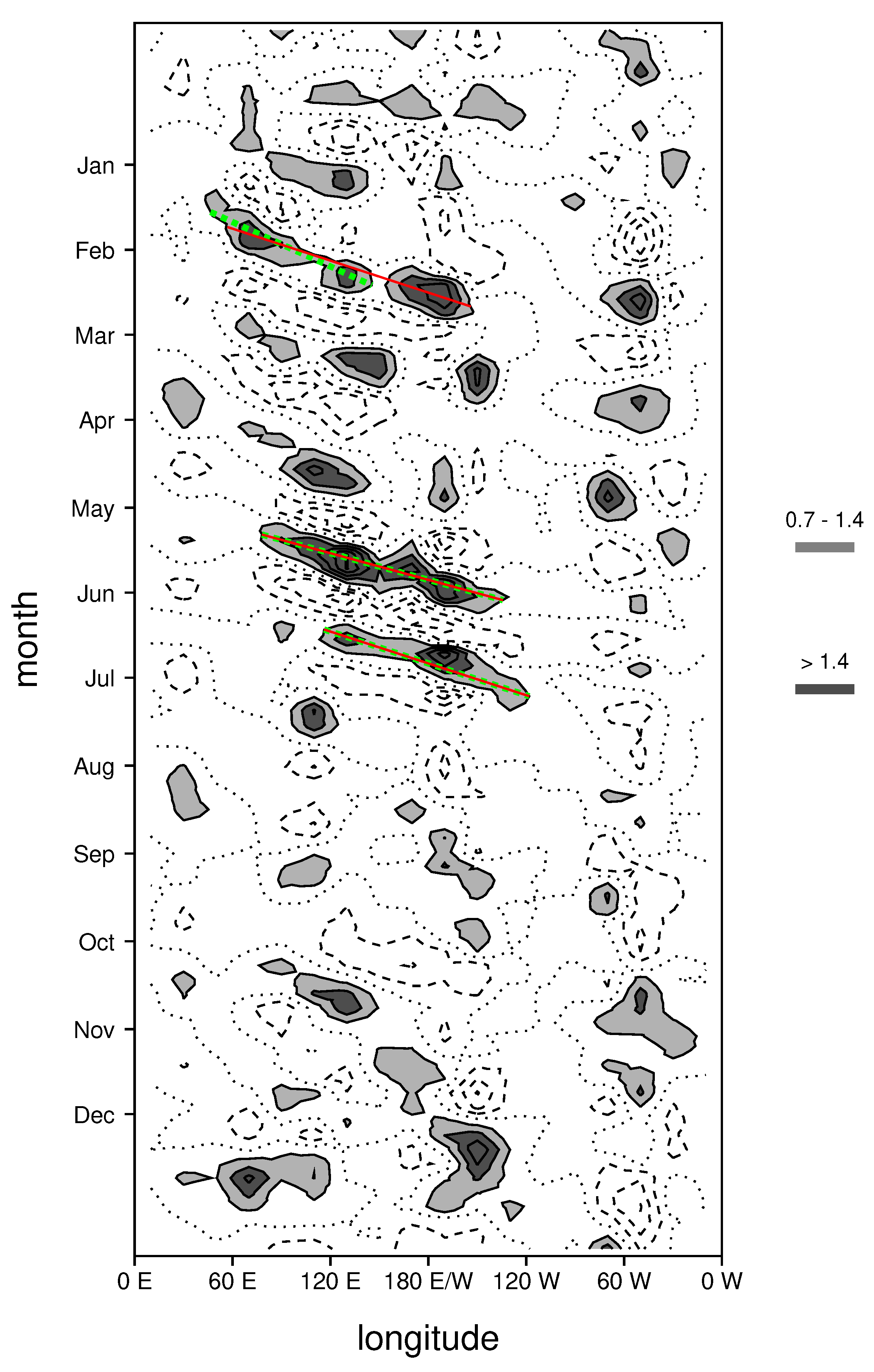
In order identify the paths of MJOs, average rainfall for 15 S to 15 N is bandpass filtered for periods between 15 and 75 days. The resulting time-longitude series of rainfall are contoured with a 0.7 mm/day contour interval (Figure 1). An object algorithm identifies contiguous eastward propagating regions of filtered rainfall that exceed 0.7 mm/day and span at least 90 degrees longitude, and it provides a linear approximation of their paths (dashed greens lines in Figure 1). In most cases these paths are used as tracks for MJOs (e.g., see the two MJOs that occur during May trough July). However, in some cases objectively identified paths miss extensions to the MJO precipitation envelope that have a small gap in rainfall that exceeds the 0.7 mm/day threshold (see February MJO in Figure 1). In such cases the MJO paths are subjectively extended to obtain a better approximation of the path of MJO rainfall (see red line for February MJO). Each linear path is then divided into thirds, to separate the initiating, mature, and dissipating stages of the convective envelope, and average vertical and horizontal structures of the MJO are constructed for each stage. A similar method was used by [6] to construct composite MJOs using satellite-derived precipitation estimates and atmospheric sounding data, and their observed MJO structure is used to evaluate the modeled MJO structure presented here; for more details on the observational MJO data the reader is referred to that study. Composite MJOs are constructed for the first and last 30 years of the LCM simulation, and comparing their structures reveals how the changing radiative forcing and associated changes in the oceanic and atmospheric basic state alter the MJO.
3. Results
3.1. LCM Basic State and Warming Patterns
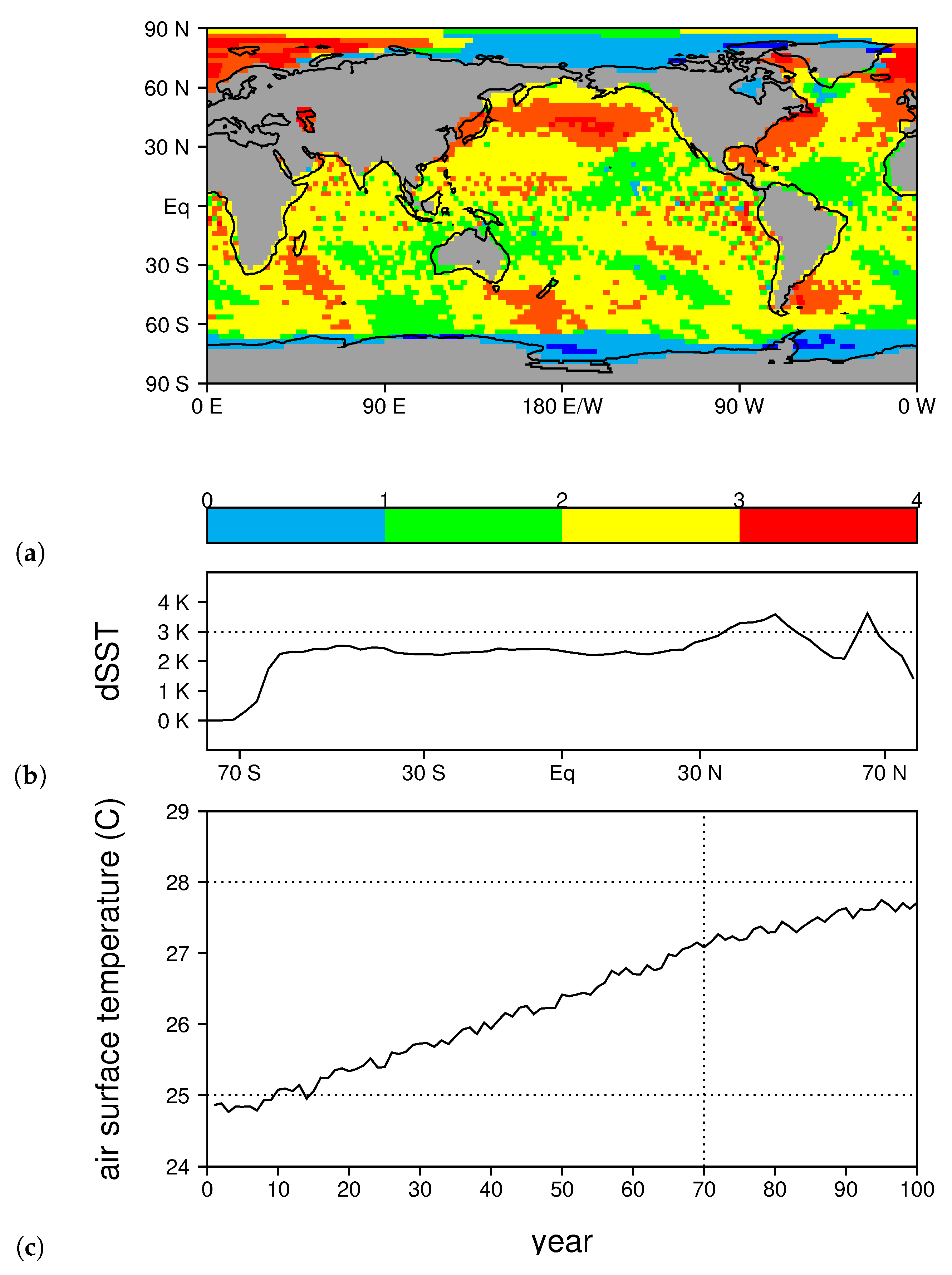
After the spin up procedure, the annual average SST pattern simulated by the LCM (Figure 2a) has the same general pattern as that observed in nature (Figure 2b). Both simulated and observed SST fields include a broad swath of warm water near the equator except in the eastern Pacific and Atlantic where cooler waters encroach from the southern hemisphere and where there is evidence of equatorial upwelling, cooler water in the northwest portions of the Pacific and the Atlantic, warm western boundary currents that travel poleward on the eastern edge of continents in the subtropics, and a region of relatively warm water to the north of Europe (Figure 2). There are a few deficiencies in the simulation including western boundary currents that separate from continents too far from the equator, a warm bias in the Southern Ocean, and a cool bias in the subtropics in the Northern Hemisphere. However, these are expected in light of the idealized equation of state used in the ocean model and its coarse resolution. Moreover, the important result for this study is that the SST pattern is sufficiently realistic to support an MJO that is very much like that observed in nature (see below), and to facilitate a study of the MJO’s longterm sensitivity to a changing radiative forcing. The ocean circulation also includes horizontal gyres, meridional overturning cells, and thermocline structure that are generally consistent with those observed in nature, but these are not sufficiently different from those presented by [38] to merit discussion here. Similarly, the general patterns of the atmospheric circulation are much like those shown in [37].
After the spin-up procedure is complete, the non-water-vapor component of the longwave optical depth is gradually increased in an attempt to simulate the effects of increases in greenhouse gases. Year 0 is defined as the time when this change in radiative forcing is implemented. The radiate forcing is increased for 70 years, and then held fixed for 30 years. The general pattern of the resulting ocean warming (Figure 3) is much like that seen in conventional climate models under high emissions scenarios. For example, compare Figure 3 with Figure 2a from [41], which shows the average ocean warming at the end of the 21st century for 28 CMIP5 models run under the RCP8.5 climate change scenario. For both the LCM and the CMIP5 composite, ocean warming is enhanced in the northern Pacific Ocean, to the east of North America, to the north of Europe, and in swaths extending east or southeastward from the southern tips of continents in the Southern Hemisphere (Figure 3a). Both kinds of models predict much less ocean warming near Antarctica, to the south of Greenland, and to the north of Siberia and North America. These results suggest that the LCM is producing a reasonable pattern of ocean surface warming, making it suitable for predicting how the MJO might change in response to our planet’s changing radiative forcing. The amplitudes of the SST increase over the 100 year simulation (Figure 3a,b), as well as the increase in surface air temperature in the tropics (Figure 3c) are also comparable to those seen in conventional climate models with similar changes to radiative forcing.
3.2. Comparing Simulated and Observed MJOs
The LCM typically produces several MJOs per year (Figure 4a), consistent with what [6] observed in nature using a similar MJO compositing approach. The frequency of MJO occurrence generally increases during the coarse of the simulation. During the first half of the simulation there are an average of 2.74 MJOs per year, and during the second half of the simulation there are an average of 3.74 MJOs per year (Figure 4a). The standard deviation in the average annual MJO count for each decade is also generally higher later in the simulation, increasing from an average of 1.13 in the first half of the simulation to an average of 1.56 in the second half of the simulation (Figure 4b). This suggests that not only does the MJO become more frequent with time, but there is also greater variability in the number of MJOs from one year to the next after the radiative forcing is modified. During the two decades of finer-resolution model spin-up that precede the results shown in Figure 4, average annual MJO counts are 2.5 and 1.8 respectively and decadal standard deviations in MJO counts are 1.4 and 1.1 respectively, which are consistent with the general patterns shown in Figure 4.
The composite MJO time-longitude series of rainfall for the first 30 years of the LCM simulation is shown in Figure 5a. During this period of time the LCM has a radiative forcing like that in nature around the turn of the century, making a comparison to the composite MJO of [6] appropriate. The simulated rainfall pattern includes an eastward propagating positive rainfall anomaly that propagates a little more than one-third of the way around the world. Eastward-propagating negative rainfall anomalies precede and trail the positive anomaly. The positive rainfall anomaly has two local maxima, roughly 30 degrees east and west of the center of the MJO path (Figure 5a). The first of these is trailed by an enhanced negative rainfall anomaly roughly twenty days later. Each of these features of the simulated rainfall time series is also present in the observed composite of [6] shown in Figure 5b. The main difference between the simulated and observed composites is that the LCM MJO propagates slightly faster than the observed MJO, which also leads to a slightly smaller period.
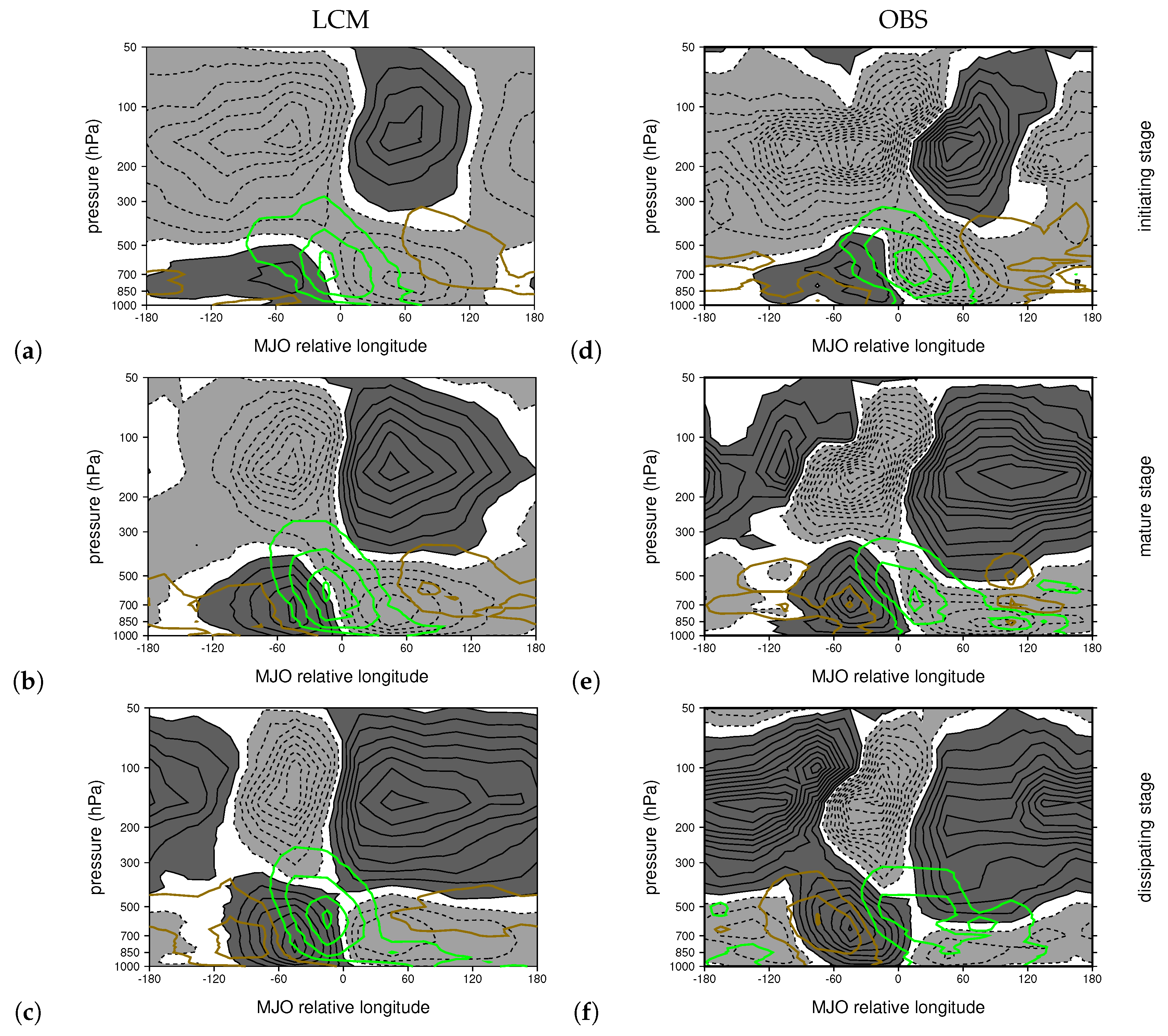
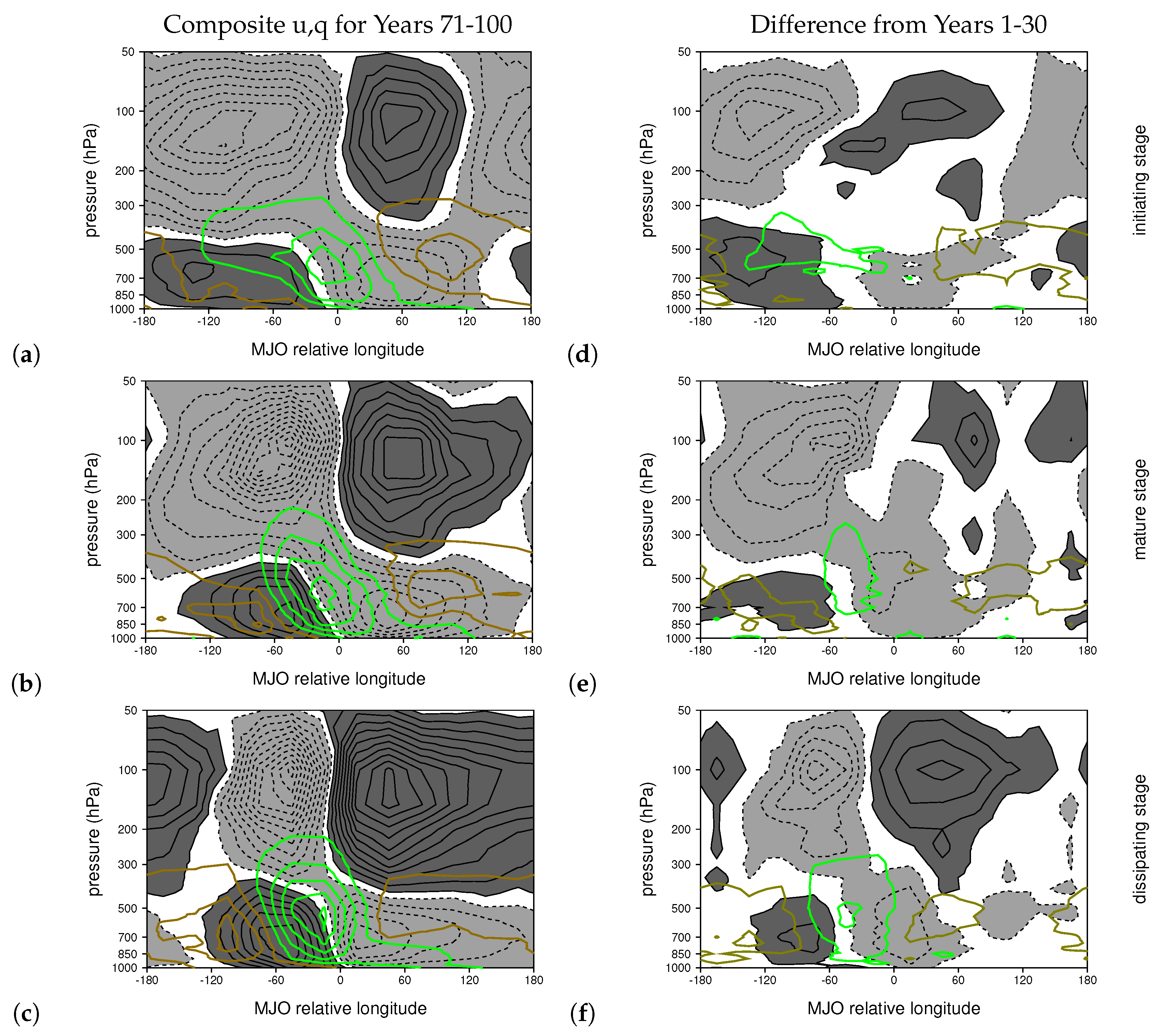
Figure 6 compares the simulated and observed composite vertical structures of MJO zonal wind and moisture perturbations. In this figure the simulated fields are shown on the left, and the observed fields are shown on the right. The first row is for the initiating stage, the second row for the mature stage, and the third row for the dissipating stage. Scanning this figure for light and dark gray shading reveals that the LCM reproduces the observed evolution of the vertical structure of zonal wind. Initially, upper-level flow is predominantly easterly (light gray shading) with a narrow band of westerlies centered about 60 degrees east of the MJO convective center which is located at longitude 0 (dark shading; Figure 6a,d). Over time, upper-level winds transition to become primarily westerly with a narrow band of easterlies just to the west of the convective center (Figure 6c,f). At low levels, there is a broad region of westerlies to the west of the convective center in the initiating stage (Figure 6a,d) that deepens and becomes more narrow later in the MJO’s life cycle in both the simulated and observed composite (Figure 6c,f). Low-level easterlies to the east of the convective center are initially narrow (Figure 6a,d), but span a broader longitude range over time in both the simulated and observed composite (Figure 6c,f). Throughout the convective life cycle there are strong low-level mosture perturbations (green contours) near the convective center that are shallower (deeper) to the east (west). Dry perturbations (gold contours in Figure 6) are initially stronger and deeper on the east side of the convective center, but later there are deep and intense dry perturbations centered just to the west of the strongest low-level westerlies (Figure 6c,f).
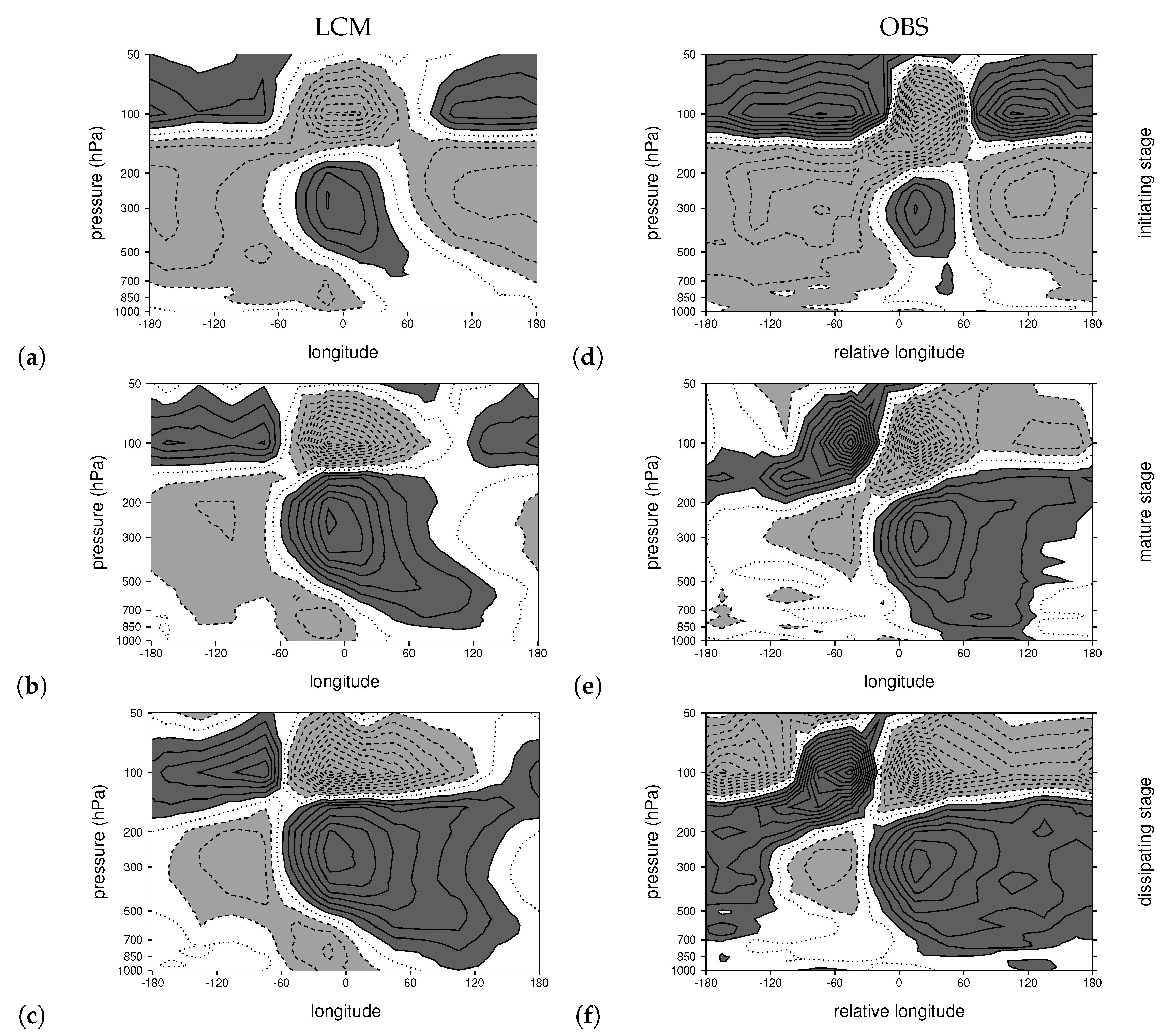
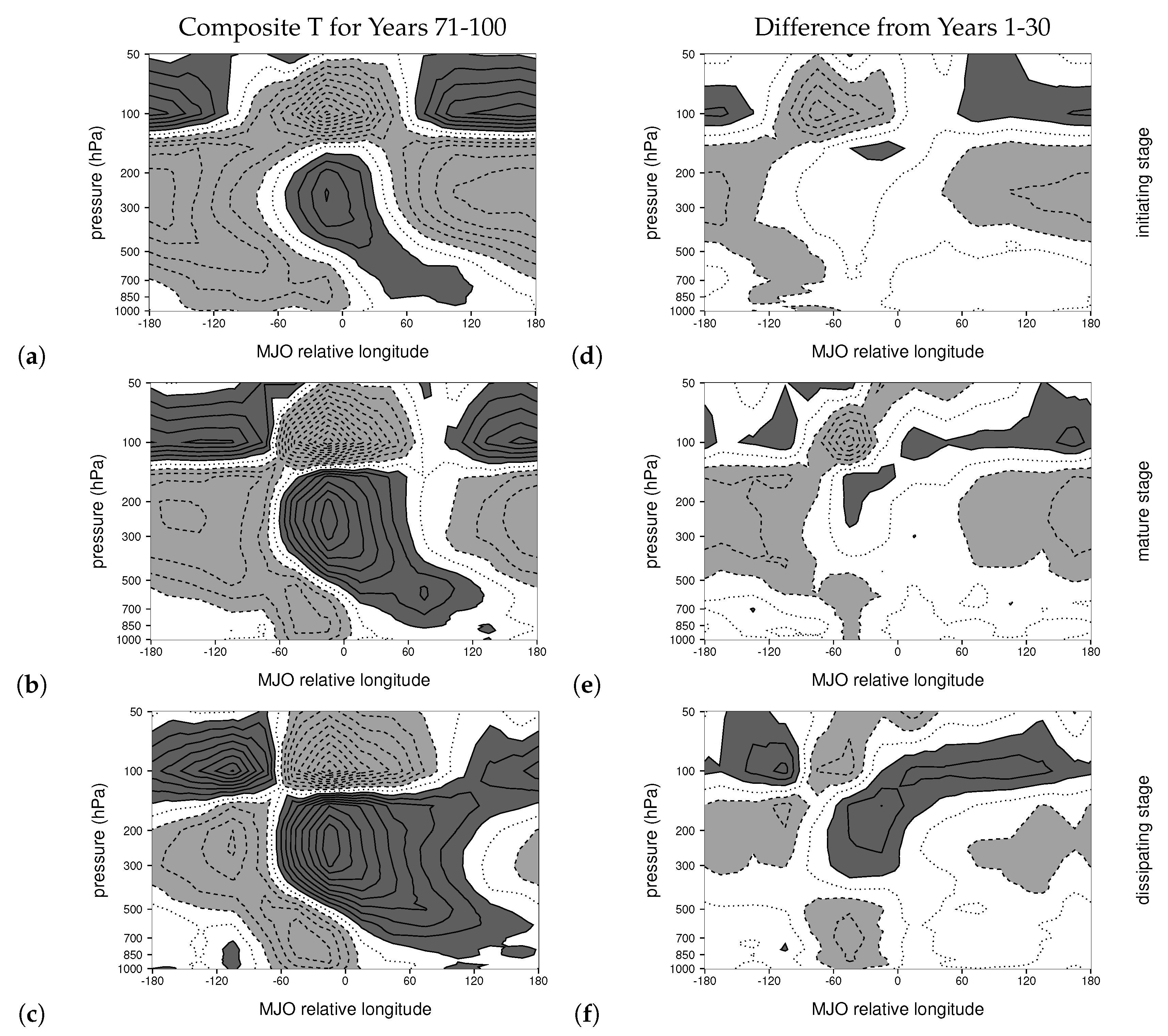
The LCM also reproduces the observed evolution of temperature perturbations (Figure 7). During the initiating stage most of the equatorial troposphere is cool, except for an upper-level warm perturbation near the MJO’s convective center (Figure 7a,d). In both the LCM and in nature the warm perturbation then spreads eastward and becomes deeper over time (Figure 7b,c,e,f). The warm perturbation spreads over a greater longitude range in nature, which could be a result of the longer period of the observed MJO (e.g., see the discussion in [6] about the warm Kelvin wave that grows eastward out of the MJO’s convective heating). By the dissipating stage most of the troposphere is relatively warm expect for a small region to the west of the MJO’s convective center (Figure 7c,f). Temperature perturbations in the lower stratosphere are generally out of phase with upper-tropospheric temperature perturbations throughout the MJO’s convective life cycle (Figure 7).
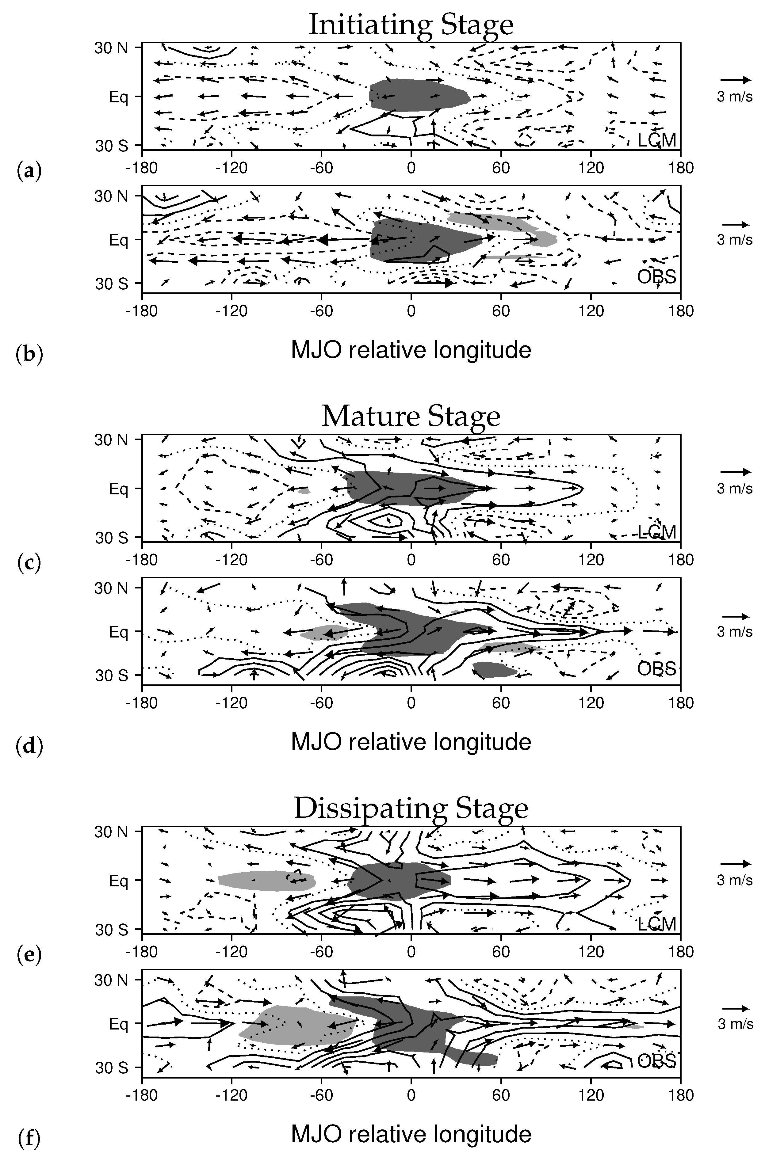
The interplay between equatorial Kelvin waves and Rossby waves in the LCM is also similar to that in nature. Figure 8 shows the horizontal structure of mean tropospheric temperature (contours) and the upper-level flow field for each stage of the MJO. In both the LCM and in nature, during the initiating stage there is a negative phase equatorial Kelvin wave spanning about half way around the world to the west of the MJO’s convective center, which includes negative temperature perturbations and easterly upper-level flow in a narrow equatorial band (Figure 8a,b). Upward motion on the leading edge of this wave likely helps to initiate MJO convection. Over time Rossby gyres form to the west of the convective center, and a warm phase Kelvin wave grows out of the east side of the convective center (Figure 8c–f).
We conclude that the LCM captures the observed MJO rainfall pattern, vertical structure, and horizontal structure, making it a suitable tool for predicting future changes to the MJO.
3.3. Changes to the MJO
We now consider how the MJO changes during the coarse of the simulation in response to a changing radiative forcing and a changing basic state. We compare the composite structure of the MJO for the last 30 years of the simulation (after the radiative forcing is fully modified), to that for the first 30 years of the simulation, which as we show above is very much like that of the recently observed MJO. These results reveal that not only does the MJO become more frequent (Figure 4), but its composite structure is also more intense in terms of rainfall, wind, moisture, and temperature perturbations. Moreover, there are a few noteworthy changes to the MJO’s dynamical structure.
The composite MJO rainfall time series for the last 30 years of the simulation shows more intense rainfall, a larger convective envelope, and a broader longitude range covered by MJO rainfall anomalies (compare Figure 9a and Figure 5a). The eastward-propagating dry anomalies that precede and trail the convective envelope are also larger and more intense. These changes, along with a decrease in period, are also evident in the difference field between the two rainfall time series (Figure 9b). The rainfall also becomes more intense later in the convective life cycle (Figure 9a,b). Finally, we note that the difference field shows stronger positive rainfall anomalies 25–30 days prior to and after the main convective envelope, suggesting that MJOs have more of a tendency to occur in series later in the simulation [42].
Later in the simulation, the composite MJO zonal wind perturbations also grow stronger (Figure 10). The greatest changes occur in the low-level westerlies and upper-level easterlies to the west of the MJO convective center. During the initiation stage, these are stronger from about 120 degrees east of the convective center, to about 50 degrees west of the convective center (Figure 10a,d) which indicates that the equatorial Kelvin wave that helps to initiate MJO convection is stronger. The difference field also indicates an increase and slight westward shift in the low-level (upper-level) zonal convergence (divergence) near the convective center. Moisture pertrubations of both signs are stronger, with greater low-level moisture near and to the west of the convective center during each phase, and greater dryness ahead of the MJO in intiation phase (Figure 10d) and trailing the MJO in the dissipation stage (Figure 10f). The changes in moisture perturbations are generally the greatest in the middle of the troposphere (Figure 10d–f), and they are located where one would expect the Kelvin wave circulation to cause moistening or drying owing to vertical motion, with positive (negative) moisture anomalies on the leading edge of low-level westerlies and upper-level easterlies (low-level easterlies and upper-level westerlies).
Composite MJO temperature perturbations for the last 30 years of the simulation (Figure 11a–c) are highly correlated with the difference field (Figure 11d–f) suggesting that the main change in MJO temperature perturbations is an overall increase in intensity. The greatest temperature change occurs in the cool anomaly extending from about 60 degrees east of the convective center to about 60 degrees west of the convective center during the initiation and mature stages (Figure 11d,e). These negative temperature perturbations overlap low-level westerlies and upper-level easterlies to the west of the convective center (Figure 10a,b,d,e), which is additional evidence that negative phase equatorial Kelvin wave to the west of the MJO convective center is stronger at later times.
The main change in the horizontal structure of the MJO late in the simulation is an increase in the strength of the Kelvin wave to the west of the MJO’s convection during the initiation and mature stages (Figure 12a–d and Figure 8a,c). This is evident in the enhancement of the cool perturbation in average tropospheric temperature and accompanying upper-level easterlies to the west of the MJO’s convection along the equator (Figure 12a–d). During the dissipating stage the Rossby gyres to the west of the MJO’s convection are also more intense and centered slightly farther west (Figure 12e,f and Figure 8e).
Table 1 shows a statitical comparison of MJO composite vertical structure fields between Years 1–30 and Years 71–100. Pattern correlation (Pearson product-moment coefficient of linear correlation) and the change in amplitude as measured by the percentage change in the standard deviation of perturbations are shown for each field. For each of zonal wind, temperature, and moisture perturbations, and for every stage, the pattern correlation between fields at the beginning and end of the simulation is 0.92 or greater, suggesting that MJO vertical structure does not undergo dramatic changes. All fields increase in amplitude, with values ranging between 15% and 40%. The greatest amplitude increase for dynamical fields is during the initiating stage, which is additional evidence that the circumnavigating Kelvin wave is much stronger later in the simulation. The greatest change in moisture is during the dissipating stage, suggesting that residual moisture after an MJO persists longer later in the simulation. The pattern correlation between rainfall time series at the beginning and end of the simulation is 0.92, with a 15 percent amplitude increase. Overall these statistics reveal that a robust strengthening of the MJO occurs in response to the change in radiative forcing.
4. Discussion
The simulations presented in this paper further support the growing body of evidence that the MJO is intensifying and will continue to intensify as the climate warms [24,25,26,27,28,29,30,31,32,33]. Aspects of predicted or observed MJO changes that the coupled Lagrangian simulation shares with other studies include heavier rainfall, more rapid propagation, and a higher frequency of occurrence. One way in which LCM simulations differ from some of those conducted with conventional climate models is that in the LCM all aspects of MJO circulations intensify including wind, moisture, and temperature perturbations (Figure 9, Figure 10, Figure 11 and Figure 12, Table 1), whereas in some climate models MJO wind perturbations do not intensify, or even weaken, when MJO rainfall becomes heavier [33].
The LCM simulations presented here also highlight a dynamical change to the MJO that is not emphasized by other studies. The most prominant change to MJO structure in the LCM is an enhancement of the cool phase Kelvin wave that lies to the west of MJO convection during the initiating and mature stages (Figure 10, Figure 11 and Figure 12). This wave includes upper-level easterlies, low-level westeries and a negative tropospheric temperature anomaly. Previous studies suggest this Kelvin wave plays an important role in initiating MJO convection and contributing to its cyclical nature [6,43]. An enhanced Kelvin wave circulation could result from a stronger oscillation in convective heating, ultimately driven by greater evaporation over warming oceans [32].The stronger Kelvin wave could also be related to the higher standard deviation in the number of MJOs per year later in the LCM simulation (Figure 4). In other words, MJOs are more likely to occur in series when stronger circumnavigating Kelvin waves of boths signs act to initiate and dissipate convection [6].
This study is a sequel to Haertel [32], hereafter H18, which discusses how the MJO changes with ocean warming in a Lagrangian atmospheric model (LAM) with prescribed SSTs. Including ocean coupling and a changing radiative forcing leads to many of the same MJO changes seen in H18. This result supports the idea that these changes are largely driven by enhanced evaporation over a warming sea surface owing to the non-linear nature of the Clausius Clapyron equation as is documented by H18. Enhanced evaporation by MJO wind perturbations leads to more moisture converging in the convective center, fuelling heavier rainfall (H18). It also leads to stronger vertical and meridional gradients in basic state moisture. There is at least one way in which the MJO changes in the LCM differ from the simulations of H18, however. When ocean coupling is included the dissipation locations of the MJO do not change substantially from the beginning to the end of the simulation, whereas in the H18 the MJO propagates farther eastward over warmer oceans. This seems to stem from the fact that the equatorial ocean warming in the LCM is weaker just east of the date line (i.e., the cold tongue effectively extends slighter farther west at the end of the LCM simulation).
The changes in the MJO that the LCM simulates in response to altered radiative forcing would likely have important impacts on other weather around the world. For example, the MJO is well known to modulate tropical cyclones [8] and monsoon disturbances [44]. If the MJO’s rainfall, moisture, and wind perturbations intensify, a stronger modulation of these cyclonic convective systems is likely, as they are known to be sensitive to horizontal and vertical wind shear as well as the saturation fraction of the atmosphere. Moreover, the structural changes in the MJO simulated by the LCM, especially the stronger cool phase Kelvin wave associated with its initiation and cyclical occurrence, could lead to occasional years with a series of five or more strong MJOs. Not only could these years have more extreme flooding and tropical cyclones than other years, but enhanced westerly wind bursts and tropical cyclones shedded from MJOs have the potential to trigger El Niños [11,12].
5. Conclusions
This study assesses changes in the Madden Julian Oscillation (MJO) in fully-Lagrangian coupled model (LCM) on a centenial time scale that stem from a changing radiative forcing. As non-water-vapor long wave depth is increased to model the effects of higher concentrations of greenhouse gases, the oceans warm, and the MJO becomes more frequent and intense and propagates more rapidly. Not only does MJO rainfall increase, but MJO wind, temperature and moisture perturbations strengthen at an even greater rate. The aspect of MJO structure that changes the most is the largely dry cool phase Kelvin wave that circumnavigates the global tropics in between moist phases of the MJO, which leads to more cyclical MJOs, and a greater standard deviation in the annual MJO count. If such changes to the MJO occur in nature, they have the potential to contribute to more extreme flooding and dry events, a stronger modulation of tropical cyclones and monsoon disturbances, and a larger stochastic atmospheric forcing of El Niñoos.
Funding
This research was supported by NSF grant AGS-1561066.
Acknowledgments
The author thanks two anonymous reviewers for their comments and suggestions.
Conflicts of Interest
The author declares no conflict of interest. The funders had no role in the design of the study; in the collection, analyses, or interpretation of data; in the writing of the manuscript, or in the decision to publish the results.
References
- Madden, R.A.; Julian, P.R. Observations of the 40–50-day tropical oscillation—A review. Mon. Weather Rev. 1994, 122, 814–837. [Google Scholar] [CrossRef]
- Zhang, C. Madden-julian oscillation. Rev. Geophys. 2005, 43. [Google Scholar] [CrossRef] [Green Version]
- Kiladis, G.N.; Straub, K.H.; Haertel, P.T. Zonal and vertical structure of the Madden–Julian oscillation. J. Atmos. Sci. 2005, 62, 2790–2809. [Google Scholar] [CrossRef]
- Nakazawa, T. Tropical super clusters within intraseasonal variations over the western Pacific. J. Meteorol. Soc. Jpn. Ser. II 1988, 66, 823–839. [Google Scholar] [CrossRef] [Green Version]
- Wheeler, M.; Kiladis, G.N.; Webster, P.J. Large-scale dynamical fields associated with convectively coupled equatorial waves. J. Atmos. Sci. 2000, 57, 613–640. [Google Scholar] [CrossRef] [Green Version]
- Haertel, P.; Straub, K.; Budsock, A. Transforming circumnavigating Kelvin waves that initiate and dissipate the Madden–Julian Oscillation. Q. J. R. Meteorol. Soc. 2015, 141, 1586–1602. [Google Scholar] [CrossRef]
- Wheeler, M.; Kiladis, G.N. Convectively coupled equatorial waves: Analysis of clouds and temperature in the wavenumber–frequency domain. J. Atmos. Sci. 1999, 56, 374–399. [Google Scholar] [CrossRef]
- Maloney, E.D.; Hartmann, D.L. Modulation of eastern North Pacific hurricanes by the Madden–Julian oscillation. J. Clim. 2000, 13, 1451–1460. [Google Scholar] [CrossRef]
- Wu, M.L.C.; Schubert, S.; Huang, N.E. The development of the South Asian summer monsoon and the intraseasonal oscillation. J. Clim. 1999, 12, 2054–2075. [Google Scholar] [CrossRef]
- Lorenz, D.J.; Hartmann, D.L. The effect of the MJO on the North American monsoon. J. Clim. 2006, 19, 333–343. [Google Scholar] [CrossRef] [Green Version]
- McPhaden, M.J. Evolution of the 2002/03 El Niño. Bull. Am. Meteorol. Soc. 2004, 85, 677–696. [Google Scholar] [CrossRef]
- Hu, S.; Fedorov, A.V.; Lengaigne, M.; Guilyardi, E. The impact of westerly wind bursts on the diversity and predictability of El Niño events: An ocean energetics perspective. Geophys. Res. Lett. 2014, 41, 4654–4663. [Google Scholar] [CrossRef]
- Emanuel, K.A. An air-sea interaction model of intraseasonal oscillations in the tropics. J. Atmos. Sci. 1987, 44, 2324–2340. [Google Scholar] [CrossRef] [Green Version]
- Sobel, A.; Maloney, E. Moisture modes and the eastward propagation of the MJO. J. Atmos. Sci. 2013, 70, 187–192. [Google Scholar] [CrossRef] [Green Version]
- Wang, B.; Rui, H. Dynamics of the coupled moist Kelvin–Rossby wave on an equatorial β-plane. J. Atmos. Sci. 1990, 47, 397–413. [Google Scholar] [CrossRef] [Green Version]
- Raymond, D.J. A new model of the Madden–Julian oscillation. J. Atmos. Sci. 2001, 58, 2807–2819. [Google Scholar] [CrossRef]
- Biello, J.A.; Majda, A.J.; Moncrieff, M.W. Meridional momentum flux and superrotation in the multiscale IPESD MJO model. J. Atmos. Sci. 2007, 64, 1636–1651. [Google Scholar] [CrossRef] [Green Version]
- Straus, D.M.; Lindzen, R.S. Planetary-scale baroclinic instability and the MJO. J. Atmos. Sci. 2000, 57, 3609–3626. [Google Scholar] [CrossRef]
- Lin, J.L.; Kiladis, G.N.; Mapes, B.E.; Weickmann, K.M.; Sperber, K.R.; Lin, W.; Wheeler, M.C.; Schubert, S.D.; Del Genio, A.; Donner, L.J.; et al. Tropical intraseasonal variability in 14 IPCC AR4 climate models. Part I: Convective signals. J. Clim. 2006, 19, 2665–2690. [Google Scholar] [CrossRef] [Green Version]
- Hung, M.P.; Lin, J.L.; Wang, W.; Kim, D.; Shinoda, T.; Weaver, S.J. MJO and convectively coupled equatorial waves simulated by CMIP5 climate models. J. Clim. 2013, 26, 6185–6214. [Google Scholar] [CrossRef]
- Grabowski, W.W. Coupling cloud processes with the large-scale dynamics using the cloud-resolving convection parameterization (CRCP). J. Atmos. Sci. 2001, 58, 978–997. [Google Scholar] [CrossRef] [Green Version]
- Kim, D.; Sobel, A.H.; Maloney, E.D.; Frierson, D.M.; Kang, I.S. A systematic relationship between intraseasonal variability and mean state bias in AGCM simulations. J. Clim. 2011, 24, 5506–5520. [Google Scholar] [CrossRef]
- Janiga, M.A.; Schreck, C.J., III; Ridout, J.A.; Flatau, M.; Barton, N.P.; Metzger, E.J.; Reynolds, C.A. Subseasonal forecasts of convectively coupled equatorial waves and the MJO: Activity and predictive skill. Mon. Weather Rev. 2018, 146, 2337–2360. [Google Scholar] [CrossRef] [Green Version]
- Slingo, J.; Rowell, D.; Sperber, K.; Nortley, F. On the predictability of the interannual behaviour of the Madden-Julian Oscillation and its relationship with El Niño. Q. J. R. Meteorol. Soc. 1999, 125, 583–609. [Google Scholar] [CrossRef]
- Oliver, E.C.; Thompson, K.R. A reconstruction of Madden–Julian Oscillation variability from 1905 to 2008. J. Clim. 2011, 25, 1996–2019. [Google Scholar] [CrossRef] [Green Version]
- Jones, C.; Carvalho, L.M. Changes in the activity of the Madden–Julian oscillation during 1958–2004. J. Clim. 2006, 19, 6353–6370. [Google Scholar] [CrossRef] [Green Version]
- Arnold, N.P.; Branson, M.; Kuang, Z.; Randall, D.A.; Tziperman, E. MJO intensification with warming in the superparameterized CESM. J. Clim. 2015, 28, 2706–2724. [Google Scholar] [CrossRef]
- Takahashi, C.; Sato, N.; Seiki, A.; Yoneyama, K.; Shirooka, R. Projected future change of MJO and its extratropical teleconnection in east Asia during the northern winter simulated in IPCC AR4 models. Sola 2011, 7, 201–204. [Google Scholar] [CrossRef] [Green Version]
- Adames, A.F.; Kim, D.; Sobel, A.H.; Del Genio, A.; Wu, J. Changes in the structure and propagation of the MJO with increasing CO2. J. Adv. Model. Earth Syst. 2017, 9, 1251–1268. [Google Scholar] [CrossRef] [Green Version]
- Carlson, H.; Caballero, R. Enhanced MJO and transition to superrotation in warm climates. J. Adv. Model. Earth Syst. 2016, 8, 304–318. [Google Scholar] [CrossRef] [Green Version]
- Jones, C.; Carvalho, L.M. Stochastic simulations of the Madden–Julian oscillation activity. Clim. Dyn. 2011, 36, 229–246. [Google Scholar] [CrossRef] [Green Version]
- Haertel, P. Sensitivity of the Madden Julian Oscillation to Ocean Warming in a Lagrangian Atmospheric Model. Climate 2018, 6, 45. [Google Scholar] [CrossRef] [Green Version]
- Maloney, E.D.; Adames, Á.F.; Bui, H.X. Madden–Julian oscillation changes under anthropogenic warming. Nat. Clim. Chang. 2019, 9, 26–33. [Google Scholar] [CrossRef]
- Pritchard, M.S.; Bretherton, C.S. Causal evidence that rotational moisture advection is critical to the superparameterized Madden–Julian oscillation. J. Atmos. Sci. 2014, 71, 800–815. [Google Scholar] [CrossRef] [Green Version]
- Adames, Á.F.; Kim, D.; Sobel, A.H.; Del Genio, A.; Wu, J. Characterization of moist processes associated with changes in the propagation of the MJO with increasing CO2. J. Adv. Model. Earth Syst. 2017, 9, 2946–2967. [Google Scholar] [CrossRef] [PubMed] [Green Version]
- Haertel, P.; Straub, K.; Fedorov, A. Lagrangian overturning and the Madden–Julian Oscillation. Q. J. R. Meteorol. Soc. 2014, 140, 1344–1361. [Google Scholar] [CrossRef]
- Haertel, P.; Boos, W.R.; Straub, K. Origins of Moist Air in Global Lagrangian Simulations of the Madden–Julian Oscillation. Atmosphere 2017, 8, 158. [Google Scholar] [CrossRef] [Green Version]
- Haertel, P. A Lagrangian Ocean Model for Climate Studies. Climate 2019, 7, 41. [Google Scholar] [CrossRef] [Green Version]
- Guan, B.; Waliser, D.E.; Molotch, N.P.; Fetzer, E.J.; Neiman, P.J. Does the Madden–Julian oscillation influence wintertime atmospheric rivers and snowpack in the Sierra Nevada? Mon. Weather Rev. 2012, 140, 325–342. [Google Scholar] [CrossRef] [Green Version]
- Haertel, P. A Lagrangian method for simulating geophysical fluids. In Lagrangian Modeling of the Atmosphere; John Wiley & Sons: Hoboken, NJ, USA, 2012; pp. 85–98. [Google Scholar]
- Mizuta, R.; Arakawa, O.; Ose, T.; Kusunoki, S.; Endo, H.; Kitoh, A. Classification of CMIP5 future climate responses by the tropical sea surface temperature changes. Sola 2014, 10, 167–171. [Google Scholar] [CrossRef] [Green Version]
- Matthews, A.J. Primary and successive events in the Madden–Julian oscillation. Q. J. R. Meteorol. Soc. 2008, 134, 439–453. [Google Scholar] [CrossRef] [Green Version]
- Powell, S.W.; Houze, R.A., Jr. Effect of dry large-scale vertical motions on initial MJO convective onset. J. Geophys. Res. Atmos. 2015, 120, 4783–4805. [Google Scholar] [CrossRef]
- Haertel, P.; Boos, W.R. Global association of the Madden-Julian Oscillation with monsoon lows and depressions. Geophys. Res. Lett. 2017, 44, 8065–8074. [Google Scholar] [CrossRef]
Figure 1.
Illustration of the compositing method. Band pass (15–75 days) filtered rainfall for 15 S to 15 N is contoured with a 0.7 mm/day contour interval. The zero contour is dotted, and values greater than 0.7 (1.4) mm/day are shaded light (dark) gray. Dotted green lines indicate potential MJOs identified by an objective algorthm; red lines shows paths of MJOs included in the composite.

Figure 2.
Comparison of simulated and observed sea surface temperatures (SSTs). (a) Annual average SST for years 1–10 of the LCM simulation. (b) Observed annual average SST from the NCEP Optimally Interpolated weekly SST and Sea Ice Data for 1998–2009.
Figure 2.
Comparison of simulated and observed sea surface temperatures (SSTs). (a) Annual average SST for years 1–10 of the LCM simulation. (b) Observed annual average SST from the NCEP Optimally Interpolated weekly SST and Sea Ice Data for 1998–2009.

Figure 3.
Metrics of global warming. (a) Difference in average sea surface temperature (SST) between Years 1–10 and Years 91–100 (C). (b) Longitudinal average of panel (a). (c) Average surface air temperature over 30 S to 30 N. The vertical dotted line in panel (c) indicates when the non-water-vapor longwave optical depth has reached its maximum value.

Figure 4.
How the frequency of occurrence of MJOs and its deviation changes by decade over the course of the simulation. (a) Average frequency of occurrence (FOC) of MJOs for each decade. (b) Standard deviation of FOC for each decade.
Figure 4.
How the frequency of occurrence of MJOs and its deviation changes by decade over the course of the simulation. (a) Average frequency of occurrence (FOC) of MJOs for each decade. (b) Standard deviation of FOC for each decade.

Figure 5.
Composite MJO rainfall time-longitude series. (a) First 30 years of the LCM simulation (15–75 day bandpass filter, 0.4 mm/day contour interval, zero contour dotted, values greater than 0.4 (1.2) mm/day shaded light (dark) gray). (b) Observed MJO from [6] (5–75 day bandpass filter, 1 mm/day contour interval, zero contour dotted, values greater than 1 (3) mm/day shaded light (dark) gray).

Figure 6.
Comparison of observed and modeled composite vertical structure of moisture and zonal wind of the MJO. (a–c) Initiating, mature, and dissipating stages in the LCM respectively for the first 30 years of the simulation. (d–f) Initiating, mature, and dissipating stages of the observed MJO respectively (from [6]). Zonal wind is contoured in black with a 0.5 m/s contour interval, with values greater than (less than) 0.25 m/s (−0.25 m/s) shaded dark (light) gray. Positive (negative) moisture perturbations are shown in green (brown) with a 0.2 g/kg contour interval (−0.7, −0.5, −0.3, −0.1, 0.1, 0.3, 0.5, 0.7 g/kg).

Figure 7.
Comparison of observed and modeled composite vertical structure of temperature of the MJO. (a–c) Initiating, mature, and dissipating stages in the LCM respectively for the first 30 years of the simulation. (d–f) Initiating, mature, and dissipating stages of the observed MJO respectively (from [6]). Temperature perturbations are contoured with a 0.1 K contour interval, with values greater than (less than) 0.1 K (−0.1 K) shaded dark (light) gray.

Figure 8.
Horizontal structure of simulated and observed composite MJOs. (a,b) Initiating stage structure for LCM and observations respectively. (c,d) Mature stage structure for LCM and observations respectively. (e,f) Initiating stage structure for LCM and observations respectively. In each panel average tropospheric temperature is contoured with 0.1 K contour interval (zero dotted, negative dashed), and vectors illustrate 200 hPa flow. The observed MJO structure is adapted from [6].

Figure 9.
Change in MJO composite rainfall time series during the simulation. (a) Composite MJO rainfall for Years 71–100 (contoured as in Figure 5a). (b) Difference between the composite rainfall for Years 71–100 and that for Years 1–30 (0.2 mm/day contour interval, values greater than 0.2 mm/day shaded light gray).

Figure 10.
The change in MJO zonal wind and moisture perturbations during the course of the simulation. (a–c) Year 71–100 composite MJO zonal wind and moisture perturbations for the initiating, mature, and dissipating stages respectively. (d–f) The difference between Year 71–100 moisture and temperature perturbations and those for Years 1–30 for the initiating, mature, and dissipating stages respectively. Zonal wind and moisture perturbations are contoured as in Figure 6.

Figure 11.
The change in MJO temperature perturbations during the course of the simulation. (a–c) Year 71–100 composite MJO temperature perturbations for the initiating, mature, and dissipating stages respectively. (d–f) The difference between Year 71–100 temperature perturbations and those for Years 1–30 for the initiating, mature, and dissipating stages respectively. Contoured as in Figure 7.

Figure 12.
The change in the composite horizontal structure of the MJO during the coarse of the simulation. (a,b) Composite MJO average tropospheric temperature and upper level wind perturbations for the initiating stage for Years 71–100 and their difference from those for years 1–30. (c,d) Composite MJO average tropospheric temperature and upper level wind perturbations for the mature stage for Years 71–100 and their difference from those for years 1–30. (e,f) Composite MJO average tropospheric temperature and upper level wind perturbations for the dissipating stage for Years 71–100 and their difference from those for years 1–30. In each panel average troposphseric temperature is contoured with 0.1 K contour interval (zero dotted, negative dashed), and vectors illustrate 200 hPa flow.


Table 1.
Pattern correlation and amplitude increase for composite MJO fields between first and last 30 years of the LCM simulation.
Table 1.
Pattern correlation and amplitude increase for composite MJO fields between first and last 30 years of the LCM simulation.
| Initiating | Mature | Dissipating | |
|---|---|---|---|
| zonal wind | 0.94, 30% | 0.95, 22% | 0.96, 25% |
| temperature | 0.93, 35% | 0.92, 18% | 0.93, 15% |
| moisture | 0.93, 33% | 0.95, 27% | 0.94, 40% |
© 2020 by the author. Licensee MDPI, Basel, Switzerland. This article is an open access article distributed under the terms and conditions of the Creative Commons Attribution (CC BY) license (http://creativecommons.org/licenses/by/4.0/).
Share and Cite
MDPI and ACS Style
Haertel, P. Prospects for Erratic and Intensifying Madden-Julian Oscillations. Climate 2020, 8, 24. https://0-doi-org.brum.beds.ac.uk/10.3390/cli8020024
AMA Style
Haertel P. Prospects for Erratic and Intensifying Madden-Julian Oscillations. Climate. 2020; 8(2):24. https://0-doi-org.brum.beds.ac.uk/10.3390/cli8020024
Chicago/Turabian StyleHaertel, Patrick. 2020. "Prospects for Erratic and Intensifying Madden-Julian Oscillations" Climate 8, no. 2: 24. https://0-doi-org.brum.beds.ac.uk/10.3390/cli8020024
Note that from the first issue of 2016, this journal uses article numbers instead of page numbers. See further details here.