Analysis of Anomalies and Trends of Climate Change Indices in Zacatecas, Mexico


Insitituto Mexicano de Tecnología del Agua - Subcoordinación de Hidrología Superficial - Paseo Cuahunáhuac 8532, Col. Progreso, Jiutepec 62550, Morelos, Mexico
*
Author to whom correspondence should be addressed.
Climate 2020, 8(4), 55; https://0-doi-org.brum.beds.ac.uk/10.3390/cli8040055
Submission received: 12 March 2020
/
Revised: 9 April 2020
/
Accepted: 10 April 2020
/
Published: 11 April 2020
Abstract
:Sufficient evidence is currently available to demonstrate the reality of the warming of our planet’s climate system. Global warming has different effects on climate at the regional and local levels. The detection of changes in extreme events using instrumental data provides further evidence of such warming and allows for the characterization of its local manifestations. The present study analyzes changes in temperature and precipitation extremes in the Mexican state of Zacatecas using climate change indices developed by the Expert Team on Climate Change Detection and Indices (ETCCDI). We studied a 40-year period (1976–2015) using annual and seasonal time series. Maximum and minimum temperature data were used, as well as precipitation statistics from the Mexican climatology database (CLICOM) provided by the Mexican Meteorological Service. Weather stations with at least 80% of data availability for the selected study period were selected; these databases were subjected to quality control, homogenization, and data filling using Climatol, which runs in the R programming language. These homogenized series were used to obtain daily grids of the three variables at a resolution of 1.3 km. Results reveal important changes in temperature-related indices, such as the increase in maximum temperature and the decrease in minimum temperature. Irregular variability was observed in the case of precipitation, which could be associated with low-frequency oscillations such as the Pacific Decadal Oscillation and the El Niño–Southern Oscillation. The possible impact of these changes in temperature and the increased irregularity of precipitation could have a negative impact on the agricultural sector, especially given that the state of Zacatecas is the largest national bean producer. The most important problems in the short term will be related to the difficulty of adapting to these rapid changes and the new climate scenario, which will pose new challenges in the future.
Keywords:
climate change; global warming; climate extremes; temperature; precipitation; anomalies; trends
1. Introduction
Adapting to climate change and mitigating its negative effects is today one of the most important challenges for humankind [1,2]. The Intergovernmental Panel on Climate Change (IPCC) has confirmed that human influence on the climate system is evident and increasing, and its adverse effects can be witnessed in every continent and every ocean. Additionally, the Panel states that the larger the human-related disturbance on climate, the higher the risks of serious, generalized, and irreversible impacts on people and ecosystems and the longer lasting the changes in each of the components of the climate system [3].
Climate change refers to “a change in the state of the climate that can be identified (e.g., by using statistical tests) by changes in the mean and/or the variability of its properties, and that persists for an extended period, typically decades or longer” [4]. Climate change can be a consequence of nature’s internal processes or the effect of external forces, such as modulations associated with solar cycles, volcanic eruptions, or persistent anthropogenic changes affecting atmospheric composition or soil use [5,6,7,8].
The successful implementation of adaptation strategies depends to a large extent on the accurate and timely detection of changes in climate at the regional and local levels in different parts of the world [2,9]. Changes in many extreme weather and climate events have been observed since approximately 1950, some of which have been associated with human activity, such as the decrease in extreme cold temperatures, the increase in extreme warm temperatures, the increase in maximum sea levels, and the larger number of intense precipitation events in different regions [3,4,10,11].
According to the IPCC, extreme precipitation is likely to become more intense and frequent by the end of the century in most mid-latitude continental masses, and tropical humid regions as global mean and surface temperatures increase; the frequency of extreme hot temperatures is practically certain to increase, while the frequency of extreme cold temperatures will most likely decrease in most continents as global mean temperatures rise at both the daily and seasonal scales [3]. These climatic changes produce chain reactions in the Earth system and have profound effects on human and environmental systems [8], and they represent an adaptation challenge for climate-sensitive sectors such as agriculture [12], hence the need to develop management practices and systems intended to maintain agricultural productivity and avoid food security problems [13]. Although most societies and agricultural and environmental systems have historically adapted to climate extremes, they may not easily adapt to the changes represented by the tails of daily data distributions because extreme climate events often have very direct and nonlinear impacts [14]. Moreover, the adaptive capacity of some areas is limited by financial, human, and physical capital, as well as by people’s lifestyle and cultural barriers.
In this context, and due to their importance and implications for physical, human, and environmental processes, analyzing the trends of recent changes in temperature and precipitation extremes has been the focus of different studies [11,15,16]; many of the tools used in these studies to monitor changes in climate extremes have been developed using indices. These analyses are essential for a comprehensive appraisal of changes in climate extremes in specific regions or places [17].
Although there is no unambiguous definition of climate extreme, the use of a common theoretical basis to define extreme events allows for their systematic study [18]. In this regard, the Expert Team on Climate Change Detection and Indices (ETCCDI), sponsored by the Commission for Climatology (CCI) of the World Meteorological Organization (WMO), the Climate Predictability and Variability (CLIVAR) project, and the Joint Technical Commission for Oceanography and Marine Meteorology (JCOMM), developed a set of 27 indices (16 associated with temperature and 11 with precipitation) to detect changes in the behavior of climate extremes [19]. This set of indices was defined in order to calculate changes in climate extremes in exactly the same way throughout the world with the purpose of having a common global baseline [20,21]; this baseline makes it possible to compare studies carried out anywhere on the planet and encourages further research of this kind, especially in less developed countries [22].
This set of indices was used to examine changes in climate extremes in five areas of the world where regional workshops on climate change were held [23,24,25,26,27,28], and a global analysis incorporating the indices calculated in the regional workshops was also conducted [29]. Although results varied from region to region, evidence of significant changes in extreme temperatures consistent with global warming was generally found after 1950, i.e., increased maximum temperature events and decreased minimum temperature events. Precipitation-related changes showed a general and significant increase in some regions, but these changes were much less spatially coherent in comparison with temperature-related changes.
These indices have also been used in different countries to search for evidence of climate change (e.g., [30,31,32,33], among others), and results are broadly consistent with increasing trends in mean global temperature. However, precipitation-related trends are unclear, and there are significant differences from one country to another, which indicates that global changes in this climate variable are not homogeneous throughout the world, but vary from one place to another [34,35]; therefore, subnational and local studies need to be conducted in order to detect and better understand the changes taking place at a small scale, not only concerning precipitation extremes, but also temperature extremes. In the specific case of Mexico, the indices created by the ETCCDI have been used at the local level to detect possible changes in climate in a number of watersheds, states, or cities [36,37,38,39,40,41]; results are generally consistent when analyzing adjacent places or areas with similar climatic conditions, but they can differ for remote watersheds or regions with different climatic conditions. For example, in a study carried out in the state of Veracruz [36], located on the Gulf of Mexico (in the country’s southeast), results showed evidence of warmer conditions in recent years (increased frequency of hot days and decreased frequency of cool days), and precipitation was found to occur over shorter periods. These data are consistent with those obtained by another, more recent study, carried out in the cities of Xalapa and Coatepec (in the state of Veracruz), reporting that temperatures were found to be less extreme (less difference between high and low temperatures) and that total annual precipitation has increased, but it also occurs over shorter periods [39]. However, these results differ from those obtained for the Conchos river basin, located in the north of the country, in the state of Chihuahua, where results clearly indicate a significant increase in the duration of dry periods over the past years [40]. Hence the importance of carrying out local studies on extreme climate trends. Increasing the accuracy with which we detect changes taking place in different regions of the country will produce information that can be used to make sound decisions concerning the implementation of relevant adaptation and mitigation measures.
In this regard, the purpose of the present study was to analyze trends in eight climate indices proposed by the ETCCDI (four temperature indices and four precipitation indices) in the state of Zacatecas, Mexico, to detect changes in climate extremes over a 40-year period (1976–2015). The state of Zacatecas, located in a semi-arid region of importance to national agriculture, is vulnerable to the effects of extreme hydro-meteorological and climate events, such as cold fronts, heat waves, droughts, frosts, or torrential rains. The results of this study will help to determine the areas of the state that have been affected the most by climate change and to create an image of the spatio-temporal distribution of extreme temperature and precipitation events. These data will support the adaptation or development of technologies and production systems to address the present conditions.
2. Materials and Methods
2.1. Description of Study Area
The state of Zacatecas is located in the north-central region of Mexico, between coordinates 21.016 and 25.116 N and 100.716 and 104.366 W; it has a surface area of 75,284 km2, which represents 3.8% of the national territory. Its northern borders are shared with the states of Durango and Coahuila; to the east with the states of Coahuila, Nuevo León, and San Luis Potosí; to the west with Jalisco, Nayarit, and Durango; and to the south with Guanajuato, Jalisco, and Aguascalientes (Figure 1a,b). It has a population of 1.5 million inhabitants, most of whom (59%) live in urban areas, whereas the rest (41%) live in rural communities [42] (Figure 1).
The state’s topography is quite variable, including mountains, valleys, plains, and plateaus, because it is part of three different physiographic provinces: the Sierra Madre Occidental (located in the north of the state), the Sierra Madre Oriental (center and southeast), and the Central Mexican Plateau (south of the state). The minimum altitude in the state, in the Juchipila river canyon, is 840 m above sea level (masl), whereas the highest point is located on the Cerro de los Pelones, with an altitude of 3160 masl. The city of Zacatecas, the state capital, has an average altitude of 2450 masl (Figure 1b).
The predominant climate in most of Zacatecas is dry and semi-dry (73%); 17% of the territory, in the east of the state, is temperate subhumid; in 6% of the territory, mainly the north and northeast regions, the climate is very dry, and the remaining 4% of the state, in the south and southwest, presents subhumid warm climate (Figure 1c). Mean annual temperature is 17 °C, with a maximum mean temperature of 30 °C in the month of May and a minimum mean temperature of 3 °C in the month of January. Average annual precipitation is 510 mm, although the value is 300 mm in the northern part of the state and 860 mm in the south; the rainy season is in the summer (June to September). The dry and semi-dry climate of the state is a limitation for agriculture, which is irrigated and seasonal and is one of the main economic activities in the state [47].
Most of Zacatecas is located in the hydrological regions of El Salado and Lerma-Santiago (39.9% and 32.7% of the territory, respectively). These regions are located in the central and southern portions of the state, and they are characterized by their high availability of surface water and groundwater. In contrast, the Nazas-Aguanaval hydrological region, comprising a large portion of the state’s north (23.6%), is characterized by its very dry climate, which makes it most vulnerable to water scarcity. The rest of the state (3.8%) is located in the hydrological region of the Presidio-San Pedro rivers and has little influence on the state’s hydrological system (Figure 1d).
Concerning soil use and vegetation, the northern part of Zacatecas is dominated by scrubland and grassland, while the central part and small portions in the south are dominated by rainfed and irrigated agriculture. The southwestern region has a variety of vegetation types, such as forest and secondary vegetation, and gallery forest in areas close to surface currents. The use of land for urban development is still minimal in the state; the largest urbanized areas are the cities of Zacatecas and Fresnillo (Figure 1e).
2.2. Selection of Weather Stations
Weather stations from the CLImate COMputing (CLICOM) system, operated by the Mexican Meteorological Service [48], were selected to obtain data on maximum temperature (TMAX), minimum temperature (TMIN), and precipitation (PP). Selection criteria were based on recommendations by the World Meteorological Organization (WMO); thus, selected stations were those having 80% or more data available for the analysis period (1976–2015) and being located in the state of Zacatecas or within a 40-km range beyond its border in neighboring states. However, given that weather stations are scarce in some parts of the state, estimations for these areas are complicated due to the lack of data. Therefore, it was decided to use monthly reanalysis series and data (TMAX, TMIN and PP) from CRU TS (Climate Research Unit) databases (version 4.03) [49], with a resolution of 0.5° latitude by 0.5° longitude, as reference series for areas affected by information gaps. The interpolation process used was angular-distance weighting (ADW); this method provides an improvement in the plot between each grid value and the input observations. Table 1 shows the number of weather and reanalysis stations used in the data homogenization process for each variable, and the geographical location of the stations is shown in Figure 2.
2.3. Quality Control, Homogenization, and Filling of Missing Data
Changes in the observing conditions or the environment around climatological stations introduce anomalous perturbations in the data series (inhomogeneities). Therefore, homogenization is of paramount importance for a reliable analysis of the variability of the climatological series, and plenty of literature and software focus on the different methodologies applied so far [50,51,52]. Different types of homogenization methods may lead to different types of results. However, it has been proven that relative homogenization is the best option; in recent times, pairwise approaches have been predominant, and absolute methods are the last resort [51,52]. Therefore, among all the available options, we decided to use the relative homogenization tool called Climatol (version 3.1) [53], which runs in the R programming language. Thus, quality control, homogenization, and the filling of data missing from climate databases, was carried out using this software, which is used to fill gaps in climate series and allows for the detection of anomalous values that can be due to data capture errors. Climatol has the option of using reanalysis series as a reference to nearby stations, and the software is compatible with the Paulhus and Kohler method [54], in which daily series are filled with spatially close average values. The tool normalizes data by dividing it by its mean values and subtracting the means or by complete standardization. Nevertheless, the main problem with this method is that the means of the series over the study period cannot be known if the series are incomplete, which is common with real-world data series. To solve this problem, Climatol calculates these parameters using the data available for each series, fills missing data using provisional means and standard deviations, and recalculates with the already filled series; subsequently, the data initially absent are recalculated to obtain new means and standard deviations, and the process iterates until none of the means change when data are rounded to their initial accuracy [53]. The series estimated based on the rest of the series serve as references for their corresponding observed series; thus, the next step is to determine series of anomalies by subtracting estimated values from observed values; these series are used to control the quality of the series, to eliminate anomalies exceeding a predefined threshold, and to test their homogeneity by using the standard normal homogeneity test (SNHT) [55].
2.4. Creation of An Interpolated Grid
Based on the homogenized data series, an interpolated grid was created using the dahgrid function in Climatol, which uses the inverse distance weighted (IDW) method [53]. This function generates daily grids for the user to define spatial limits and spatial resolution. In the present study, the selected spatial resolution was 0.2° (approximately 20 km). This initial resolution is relatively low when compared to the spatial surface of the state of Zacatecas, whose topography is irregular. Therefore, it was decided to create a second grid, in high resolution, using the base level temperature method [56]; this method attempts to fit the initial grid to a digital elevation model (DEM) by simply matching grid points at a unique altitude (i.e., 0 m, the average altitude of the studied region, or an altitude value defined by the user); in the present study, based on the elevation model, we used the average altitude of the state (2000 masl). The determined temperature is calculated using the following equation:
where is the daily temperature of each grid point; is the correlation coefficient between the elevation and temperature of each grid; is the determined altitude, and is the altitude of each grid point. The result is the temperature value of each grid point if it were at a certain altitude (in this case, 2000 masl). Subsequently, another calculation is performed to determine the new value of each grid point using the resolution of the digital elevation model:
where is the new temperature value assigned to the new resolution; is the same correlation coefficient previously used, and is the value of each pixel in the digital elevation model.
The result was a new, NetCDF-format grid adjusted to the topography of the study area, which allowed for a more detailed observation of the distribution of temperature in the state of Zacatecas.
2.5. Calculation of Climate Change Indices
Climate change indices were calculated using the high-resolution homogenized grid and the Climdex.pcic.ncdf software [57] at the annual and seasonal scales. Of the 27 indices proposed by the ETCCDI [58], eight (four related to temperature and four to precipitation) were selected. These indices are the most representative of the climatology of the study area; they are presented in Table 2 and described below:
1 Summer days (SU)
Annual count of days when maximum temperature (TX) is higher than 25 °C. Where TXij is the maximum temperature on day i in period j, the number of days in a year is counted when:
TXij > 25 °C
2 Frost days (FD)
Annual count of days when minimum temperature (TN) is lower than 0 °C. Where TNij is the minimum temperature on day i in period j, the number of days in a year is counted when:
TNij < 0 °C
3 Extreme maximum temperature (TXx)
Maximum seasonal value of maximum daily temperature. Where is the maximum daily temperature from station , the maximum seasonal extreme temperature is:
TXx = max(TXij)
4 Extreme Minimum Temperature (TNn)
Minimum seasonal value of minimum daily temperature. Where is the minimum temperature on day from station , the minimum extreme seasonal temperature is:
TNn = min(TXij)
5 Total precipitation on humid days (PRCPTOT)
Where is the amount of precipitation on day in period . If represents the number of days in , then:
6 Consecutive dry days (CDD)
Where is the daily amount of precipitation on day in period , the largest number of consecutive days is counted when:
CDD = RRij < 1mm
7 Daily maximum precipitation (Rx1day)
Where is total precipitation on day in period , the maximum values of one day for period are:
Rx1dayj = max(RRij)
8 Maximum consecutive 5-day precipitation (Rx5day)
Where is the amount of precipitation for the five-day interval ending in , period , the maximum 5-day values for period are:
Rx5dayj = max(RRkj)
The ETCCDI has established indices based on monthly analyses (TXx, TNn, Rx1day, Rx5day, among others). In the present study, monthly series data were grouped into seasonal series (winter, spring, summer, and fall) to identify seasons responding to variations in climate change indices concerning their input variable. For indices TXx and TNn, the months of December, January, and February (DJF) corresponded to the winter; the months of March, April, and May (MAM) to the spring; the months of June, July, and August (JJA) to the summer, and the months of September, October, and November (SON) corresponded to the fall. Precipitation indices (Rx1day and Rx5day) used a different by-month grouping for the summer and fall seasons: the months of June, July, August, and September (JJAS) corresponded to the summer, and only the months of October and November (ON) corresponded to the fall. This change was introduced with the purpose of analyzing time-related variations in precipitation patterns over the four-month period (JJAS), which accounts for approximately 80% of cumulative annual precipitation. Winter and spring months were grouped as in the case of the temperature indices (DEF and MMA).
2.6. Analysis of Indices using Hovmöller Diagrams
Hovmöller diagrams are used to represent the spatio-temporal evolution of a specific variable on two axes: time is plotted on the abscissa axis and latitude on the ordinate axis [59]. Results were also analyzed using warming stripes diagrams [60], which depict the time series and its standardized anomaly in the form of colored bars; these diagrams help to discern normal values from unusual values. Standardized anomalies (X) are defined as the difference between the recorded value (x) and the mean of the data () divided by the standard deviation of data (σ). These are dimensionless numbers; when their value is 0, they are equivalent to the mean, and when their value is 1, they are equivalent to the standard deviation of the data:
2.7. Trend Analysis by Mann–Kendall Non-parametric Rank Correlation Tests
These tests identify the presence of changes and describe whether such trends are statistically significant [61]. The level to accept a change as statistically significant was established at . Values for below this parameter were considered to be statistically significant.
The R package greenbrown is a collection of functions that can be used to analyze trends, changes in trends, and phenological events (e.g., satellite observations or climate model simulations) in time series organized as a grid [62,63]. The present study used this algorithm to understand trends and values of indices calculated from homogenized grids.
It is important to mention that the trends could be affected if serial autocorrelation is present in the time series. However, we assumed the absence of autocorrelation in the analyzed time series, although this should be verified in future studies.
3. Results
This section presents the results obtained after applying the procedures described above. An analysis of the availability of data from climate stations in the state of Zacatecas and surrounding states is presented first, then we show an example of final homogenized grid for daily maximum and minimum temperatures, followed by the climate characterization of the state of Zacatecas, and finally, the calculation of climate change indices.
3.1. Data Availability
During the period from 1976 to 2015, the amount of data available for the three variables used in quality control and homogenization was 88%. Data tended to be unavailable at the beginning and at the end of the study period (Figure 3). For example, stations within the state of Zacatecas (shown in the upper part of the three graphics) failed to provide data from the late 1980s and mid- to late 2000s, and some stations show gaps at the beginning of the period. It should be highlighted that more than 80% of the data from most stations were available for the study period; therefore, these weather stations were considered as highly important in terms of data availability, especially in view of the scarcity of recent climate information in Mexico.
3.2. High-resolution Homogenized Grid
The results obtained by calculating the base level temperature are best perceived when considering the spatial distribution of the maximum and minimum temperatures according to a digital elevation model (DEM). Factoring altitude results in a more accurate adjustment of temperature in the study region. Figure 4 shows the comparison of the maximum temperature grid generated by Climatol and the new grid, calculated using the base level temperature method. The warmest zones are located in the southwest, adjacent to the state of Jalisco, and in small northern areas bordering the states of Durango and Nayarit, whereas the most temperate zones are concentrated in the center of the state of Zacatecas.
3.3. Characteristics of Climate in the State of Zacatecas
The climate of the state of Zacatecas from 1976 to 2015 was characterized based on homogenized data to outline the annual cycles of maximum temperature, minimum temperature, and precipitation. The climograph in Figure 5 shows that the maximum temperature occurs in May (30.7 °C; spring), and the minimum temperature in January (2.3 °C; winter); the mean annual temperature is 21.6 °C. Minimum precipitation occurs in March (8 mm), and maximum precipitation in July (107.8 mm). Average precipitation is 472.7 mm per year. Precipitation was observed to be monsoon-like; that is, most of the rain falls from June to September.
In addition to the annual cycle, divided into months, seasonal average maps of the three variables used in this study over a 40-year period (1976–2015) are included below. The geographical distribution of maximum temperature shows that maximum values occur in the spring and summer, especially in the southern region, with values close to 35 °C, whereas values decrease in the central part of the state during the fall and winter seasons (Figure 6a). Maximum seasonal temperature values range from 16 to 34.1 °C, as shown in Table 3. The spatial behavior of minimum temperature presents remarkable variations across the four seasons; maximum values of minimum temperature in the summer range from 8.7 to 17.3 °C (Figure 6b; Table 3), whereas in the winter, the minimum values were found to be −5 °C (Figure 6b), with an average oscillation between −1.2 and 7.6 °C (Table 3). During the fall and spring, climate appears to be uniform; however, differences of approximately 4 °C can be observed, as shown in Table 3.
In the state of Zacatecas, precipitation is monsoonal, with the highest percentage of precipitation occurring in the summer months (June to September). Table 4 shows maximum and minimum precipitation values per season. An average of 545.5 mm per year is recorded for the summer, and the minimum annual precipitation in a season occurs in the spring, with 18.6 mm.
As indicated in a previous paragraph, maximum precipitation values in the state occur in the summer; geographically, these precipitation values are located in the southwest, decreasing gradually toward the northeast, where precipitation is lower throughout the year (Figure 7). Precipitation decreases during the fall, and its geographical distribution is similar to that of the summer (at a lower scale); this is due to the convective activity in the region and to tropical waves that persistently occur during the fall, resulting in rainfall. Precipitation is lowest during the winter and the spring, mainly due to the presence of cold fronts during the winter and early spring (Figure 7).
3.4. Climate change indices
3.4.1. Summer Days (SU)
Summer days are closely related to altitude. Summer days (when temperature is higher than 25 °C) per year are more frequent at low altitudes than at high altitudes, characterized by lower temperatures. In general, the number of summer days in Zacatecas ranges from 50 to 350, depending on the part of the state (Figure 8a). At elevations above 2000 masl, the number of summer days tends to be under 150, whereas areas under 1600 masl see more than 200 summer days per year.
The spatio-temporal analysis of summer days (Hovmöller diagram, Figure 8b) represents the evolution of this variable over time as a function of latitude in the state of Zacatecas. Areas with SU greater than 100 are mostly between latitudes 22 and 25° N, whereas the range between 15 and 90 SU is between latitudes 22 and 25° N until 1994. After 1994, SU values above 300 move north, from latitude 21° N to latitude 22° N. SU values in almost the entire state of Zacatecas are over 100 since 1994, and the years 2009 and 2011 had more than 300 summer days.
The standardized anomaly of summer days is illustrated by the diagram in Figure 8c, where important changes can be observed over the study period. From 1976 to 1993, values from 0 to −3 were recorded throughout Zacatecas, except for latitudes 24.5 and 25° N in 1979, 1982, and 1989. An important change takes place from 1994 to 2014, when anomalies acquire values from 0 to 3 throughout the state. Therefore, this index reveals two clearly differentiated periods, which is an indication of climate change (Figure 8).
The analysis of summer day trends points at a generally positive trend in the state of Zacatecas. Figure 8d shows the time series of the general average number of summer days with a slope of 2.39, which is statistically significant (p-value < 0.05). The same series shows an average increase of 150 summer days per year over 33 years (1976–2009); 2009 is the year with the largest number of summer days, and a decrease in SUs can be observed over the last three years of the series. This increased trend of summer days reflects the results of a study [38] conducted in the state of Chiapas, in southern Mexico, and the findings of another study [41] carried out in the state of Baja California, in the country’s northwest.
A thorough spatial examination of summer day trends should include the map in Figure 8e, which shows the trend slope for each grid point. Positive values were observed throughout the state (minimum of 0.07 and maximum of 3.44); the central part of the state has the highest slope values and is the most prone to an increase in the number of summer days; in the northeast region, a portion showing moderate positive values was observed, and the south region showed positive values close to zero. The statistical significance of the SU index is very high, since 99.5% of the state’s surface has a p-value under 0.05, which makes the confidence level quite high for practically the entire state (Figure 8f).
3.4.2. Frost Days (FD)
The geographical distribution of FDs in Zacatecas is shown as an annual average in Figure 9a, which also shows that the south has less than 20 days of frost on average and that the eastern and western regions have between 20 and 40 FDs. There are areas in the northeast where the values are between 60 and 80 days; the central and western regions present small cores where the highest FD values can be found, ranging from 70 to 90 FDs on average.
The spatio-temporal analysis of frost days (Hovmöller diagram, Figure 9b) shows increases in FD after 1996 between latitudes 22.5 and 24.5°N, the band with the largest number of frost days; at latitudes below 22.5° N, FD values range from 0 to 15 from 1976 to 1995 and begin to increase afterward, similar to the values at latitudes above 24.5° N in the same period. Increases in FD from 1996 onward are very significant between latitudes 22.5 and 24.5° N, where the maximum values (84 days) of the study period were recorded in 2008. A gradual decline can be observed from 2012 to 2015, when the highest FD values were recorded between latitudes 22.7 and 23.7° N; by 2015, the number of FDs had notably decreased throughout the state, in contrast with the increases beginning in 1996.
Standardized anomalies (Figure 9c) for FD in Zacatecas have a negative value in the first 20 years of the study period (1976–1995); small areas of normal values can be observed throughout the period. Since 1996, however, anomaly values become positive, with the exception of 2001 and 2015, which present normal values and a slight slope toward positive values. The year 2010 presents the highest values of positive anomalies in the state. After 2012, anomalies present positive and then normal and negative values up to 2015. An area where positive anomalies persist can be located at latitude 25°N, most notably in 2014.
When observing the linear trend (Figure 9d), the first 20 years of the study period are free of significant changes. Abrupt changes begin to occur in 1996, and variations are notable from year to year; a gradually decreasing trend can also be appreciated from 2012 to the end of the study period. In general, the FD trend in Zacatecas is unmistakably leaned toward the increase, with a statistically significant p-value (Figure 9).
The spatial trend of FD (Figure 9e) shows a positive slope in most of the state’s surface area, except for the northeast, where the slope is negative. The central region presents the highest positive slope values. In the south, the slope presents values close to zero, and as shown by the Hovmöller diagram in Figure 9b, there are no important changes in this region, where FDs are scarce because elevation in this part of the state is low in comparison with the rest of the territory, above 1800 masl. In regard to spatial statistical significance, the p-value in 90.1% of the surface can be observed to be under 0.05 (Figure 9f); additionally, the region that showed a negative trend was the area with p-values from 0.051 to 1, which resulted in a low confidence level possibly due to the sharp decrease in the number of FDs in the region, especially between 2013 and 2015.
3.4.3. Extreme Maximum Temperature (TXx)
This index was analyzed by season. Table 5 shows maximum and minimum values by season; the highest extreme temperatures occur in the spring, but high temperatures are also common in the summer, when the value is only one degree lower than that of the spring. Extreme temperatures are up to 5 °C lower in the fall and winter.
An analysis of TXx seasonal average maps (Figure 10a) reveals values between 28 and 40 °C in the spring and summer. The highest temperatures occur mainly in the south, and TXx values above 30 °C during the spring are prevalent in virtually the entire state. In the fall, TXx values range between 26 and 33 °C, and the minimum values occur in the central and eastern regions. The highest values during the fall, as with the rest of the seasons, are concentrated in the south of the state. In the winter, TXx decreases markedly in the center and toward the north of the state, with values around 24 °C, and the southern region remains warm, at temperatures as high as 33 °C; therefore, the geographic distribution of TXx runs from southwest (higher TXx) to northeast (lower TXx).
The spatio-temporal evolution of extreme maximum temperature shown in Figure 10b indicates that the highest temperatures occur in areas below 22 °N. The inter-annual behavior can also be inferred from the clearly visible winter seasons, colored in yellow, when TXx decreases by approximately 5 °C. Since 1995, the red tone intensifies with the increasing temperatures in most of the state. Other studies focusing in our study area have also reported increases in maximum temperatures observed in historical series [64,65,66,67], as well as studies performed in other regions in Mexico where maximum temperatures have increased [36,37,38,39,41,68]. The hottest years in the study period are 2009, 2010, and 2011, when temperatures close to 40 °C were recorded throughout the state.
Standardized anomalies allow for the observation of important changes in TXx behavior over the 40-year study period. Figure 10c shows very noticeable increases in temperature in all seasons during the winters of 2006, 2009, and 2011. TXx begins to increase during the spring since 1995, and 2009, 2010, and 2011 are the years with the highest extreme temperatures, not only for this season but for throughout the study period. Positive anomalies were recorded during the summer in each of the last 10 years of the period. Important positive anomalies began to be recorded during the fall since 1999, and 2009 was the warmest fall in the 40-year period; these increases in TXx suggest the presence of climate change in the state of Zacatecas (Figure 10).
The analysis of trends points at a possible increase in maximum extreme temperatures; as can be appreciated in Figure 10d, all seasons present positive trends and very high statistical significance; spatial trends show a steeper slope in the spring and summer, except for the northeast and south regions, where values are close to zero, which indicates a lack of change in these trends (Figure 10e). The winter and fall show slight positive slopes, although not as pronounced as in the case of the spring and summer. Spatial statistical significance indicates that, during the spring, summer, and fall, p-values below 0.05 occur in larger areas, which indicates that the degree of confidence is quite high (Figure 10f); in the winter, statistically significant values occur in approximately 65% of the state’s territory.
3.4.4. Extreme Minimum Temperature (TNn)
As in the case of the TXx index, the analyses of the TNn index were seasonal. Table 6 shows maximum and minimum TNn values per season. These values range from −9 to 14°C; the winter presents the lowest value, and the summer presents the highest value.
Seasonal TNn averages show that the spring, fall, and winter lean toward the cold end of the spectrum, with minimum values below 0 °C, and in comparison with the rest of the seasons, the summer has the least intense minimum temperatures. Figure 11a shows the geographical distribution of the seasonal average of TNn; the highest minimum cold temperatures are located in the southern region and are consistent with the lowest elevations in the state, whereas the lowest minimum temperatures are found in the central and northern areas, where altitudes exceed 1800 masl. Two very local areas are observed in the winter where average TNn is close to −10 °C; these areas are located in the central-western and northeastern regions, near the border with San Luis Potosi (Figure 11a).
Figure 11b shows the spatio-temporal evolution of TNn throughout the 40-year study period. Interannual variations can be appreciated in the differences between summer seasons, colored in yellow-green, and winter seasons, whose predominant color is intense blue and present the highest contrast with the summer. It should be noted that TNn values are uniform for each season at all latitudes, especially in the fall, winter, and spring, when the passage of fronts carrying cold air masses affects practically the whole state of Zacatecas. The lowest temperatures during the study period were recorded at minimum values of −16.4 °C during the winter of 1997. This was due to a very intense winter storm affecting the north and central regions of the country [69]; the entire surface area of the state of Zacatecas was affected by the storm, and very low values in terms of minimum temperature were recorded even in the lowlands. Additionally, TNn values have been decreasing in all the seasons since 1997, and values close to −15 °C were recorded in 2011; however, this has affected only the central and northern parts of the state.
Seasonal standardized anomalies reflect changes in extreme minimum temperature behavior in the state of Zacatecas. During the winter, TNn has presented a decreasing trend since 1997, when the lowest temperatures in the study period were recorded; negative anomalies and values close to the winter average were recorded in the last years of the period (Figure 11c). The spring season presents positive anomalies during the first 20 years of the study, except for 1978, which shows a negative anomaly; on the other hand, negative anomalies were observed between 2003 and 2005; after these three years of cold springs, positive anomalies were prevalent until 2012, and the lowest value of TNn for the spring was recorded in 2013. The summer presents an irregular behavior, with extreme negative and extreme positive values over a range of approximately eight years; however, the year 2015 presents the lowest value of the season. Concerning the fall, positive anomalies and normal values predominate during the first 25 years of the study. A gradual decrease in anomalies commences in 2002 and continues until 2011, with an anomaly score of −3, and 2014, with a score of −2.5; the coldest fall seasons in the 40-year study period were recorded in these two years (Figure 11c).
The general trends for the spring, fall, and winter in Zacatecas present a negative slope, whereas the summer can be considered to have a slope of zero. The p-values for the fall and winter are below 0.05, which is considered a statistically significant change; the spring and summer have p-values of 0.09 and 0.9, respectively (Figure 11d). The seasonal spatial trends in Figure 11d show a negative slope in the fall and winter in most of Zacatecas, especially in the central region; once again, the northeast region stands out for its behavior, which is different from the rest of the state, where a positive slope is consistently observed (increased TNn in the winter). In the spring, the dominant slopes are negative, although to a lesser extent than in the fall and winter, although the northeast region also has a positive slope. The summer, as was mentioned in the description of the general trend, presents slope values near zero in most of the state, which points at a lack of changes in the summer. In this regard, the results of the present study are consistent with those from studies such as [64,67,68], for the states of Zacatecas and Aguascalientes, and with those from [41], which also reports on a decrease in minimum temperatures; however, studies such as [65,66] report partially different results for the Zacatecas region.
The spatial statistical significance of TNn reveals that the fall and winter are the two seasons with most surface area (90%) where p-values are <0.05. In the spring, the most statistically significant regions are the north, center-west, east, and southwest, whose approximate total area is 50%. In the summer, a small area presents statistically significant values (approximately 5%), and the rest of Zacatecas presents p-values close to 1 (Figure 11f).
3.4.5. Total Precipitation on Humid Days (PRCPTOT)
As mentioned in the materials and methods section, the PRCPTOT index does not take into account total annual accumulated precipitation. Instead, it records days when precipitation is 1 mm or more, and as a consequence, average values decrease slightly. Average PRCPTOT shows the precipitation gradient from southwest to northwest (from 783 to 203 mm). Maximum precipitation is associated with the monsoon core, whereas the minimum precipitation is found in the semiarid zones in the northeast of the state of Zacatecas [70,71,72] (Figure 12a).
The spatial evolution of PRCPTOT over the study period shows maximum values in the south, below latitude 22° N, with a gradual decrease to the north, where minimum values occur above latitude 24.5° N (Figure 12b); these conditions can be considered as normal precipitation behavior for the state of Zacatecas. However, as part of natural variability, there are years and periods when the highest amount of precipitation increases or decreases in spatial coverage. A staggered increase in precipitation coverage can be observed over the last years of the period. Maximum values occur as far as latitude 23.5° N in the early 1990s, and subsequently, in 2004, maximum values occur at 24.5° N, and values over 700 mm were recorded for the entire state of Zacatecas in 2015 (Figure 12b). Convective activity in the region and hurricane Patricia were the most influential factors in the high humidity of this particular year. In contrast, some years, such as 1979, 1989, 1998, 2005, and 2011, were very dry in most of the state (Figure 12).
An analysis of the standardized PRCPTOT anomaly in the Hovmöller diagram in Figure 12c helps to identify humid and drought periods; three humid periods can be identified in the 40-year study period: 1990–1992, 2002–2004, and 2013–2015. In addition, a positive anomaly value was recorded in 1976, but this is because 1976 is the first year of the analyzed period, and therefore, there is no certainty as to whether it is part of a humid period encompassing previous years or a unique wet year. The analysis also identifies three periods of drought. In this regard, droughts affecting mainly the northern central region occurred from 1977 to 1982, the year 1989 was characterized by negative anomaly throughout the state, and the second important dry period was recorded from 1993 to 2001, affecting most of the central region of Mexico, where the state of Zacatecas is located. The year 2005 presented negative values too, and the most intense period in terms of drought occurred in 2011 and 2012, with precipitations below 400 mm, which resulted in severe damage to agriculture. An important point to highlight is that extreme events have become more frequent in recent years [71], as indicated by the most severe drought event, which took place in 2001, and the wettest year, recorded in 2015.
In general, precipitation trends in Zacatecas have increased in recent years, especially in the central and northern regions, although the degree of reliability is low. Figure 12d shows the general trend of PRCPTOT, which shows a positive slope. However, it is not statistically significant.
The spatial trend derived from Figure 12e indicates increased precipitation in the northern and eastern regions, where slope values are highest; in contrast, the western region and a small area in the northeast of Zacatecas show values close to zero. Negative slope values are observed in the southern region, where the highest annual PRCPTOT values are recorded, and annual PRCPTOT has likely been decreasing in recent years. The regions where statistically significant values are found, the center and the east, present the highest positive slope values (Figure 12f) and p-values under 0.05; p-values were between 0.4 and 1 in the western and southern regions.
3.4.6. Consecutive Dry Days (CDD)
Average CDD ranges from 60 to 124 days per year, and values over 100 occur in the eastern, central-western, and southern regions, where the summer months are rainy. The northern and northeastern regions have a lower amount of CDD per year because, in addition to the moisture carried by flows from the southeast, they receive precipitation during the winter due to the passage of cold fronts (Figure 13a).
CDDs and PRCPTOT are closely associated; the years with most CCDs are those when precipitation was below normal in the state of Zacatecas. Figure 13b shows the Hovmöller diagram of CDDs, where years such as 1982, 1989, 1995, 1988–2000, 2009, and 2011, saw more than 150 CDDs in most of or the entire state. Conversely, there are areas where CDDs are fewer, for example, above latitude 24.5° N. This decrease could be due to precipitation associated with cold fronts in the winter, which gradually reduces the amount of CDD per year. The years 1981 and 2015 are characterized by a drastic decrease in CDD throughout the state; however, 1981 was less rainy in comparison with 2015 (Figure 13b).
The temporal evolution of standardized CDD anomalies indicates that the frequency of these events increased in the last years of the study, affecting the entire territory. These anomalies are associated with years of severe meteorological drought (Figure 13c). The lowest values of CDD anomalies occur in wet years and periods; however, the presence of negative anomalies in a particular year cannot be used as a criterion to identify the year as wet since the variability of precipitation lacks a definite annual pattern (Figure 13).
Figure 13d shows the general trend of CDD, with a marked upward trend in the final years; however, the increase in dry days shows until 2011, when the maximum value was recorded; a noticeable decrease begins after 2011 and continues until 2015, when minimum CDD values were recorded. The spatial trends analysis indicates that CDDs increased throughout the state, with the exception of two very local areas, the first in the center-east border and the second in the northwest border; these areas have negative slopes, although slope values are close to zero in certain areas (Figure 13e). However, the spatial and temporal statistical significance of this index is low, since there are no regions where p-values are under 0.05, which decreases the confidence of hypothetical changes in CDD over the 40-year study period (Figure 13f).
3.4.7. Daily Maximum Precipitation (Rx1day)
As previously indicated, in the present study, seasonal analyses of precipitation used the following seasonal grouping: spring (March, April, and May), summer (June, July, August, and September), fall (October and November), and winter (December, January, and February). The summer comprises four months because these are the rainiest months of the year, and this grouping reveals the evolution and changes of precipitation during the humid season throughout the study period. Table 7 shows the minimum and maximum values of maximum precipitation in one day by season; the summer has the highest amount of precipitation, followed by the fall and winter. The last two seasons combine rainy weather and the passage of cold fronts from the north [72].
In Figure 14, the geographical distribution of average daily maximum precipitation varies significantly from season to season. In the spring, maximum values are located in the northeast region (15.8 mm) in areas affected by frontal systems. In the summer, the gradient of maximum values is reversed (maximum values are found in the southeast) due to moisture fluxes from the Pacific Ocean; in addition, Zacatecas is exposed to the trajectories of low-intensity tropical cyclones in the summer. In the fall months (October and November), the spatial behavior of the Rx1day index is similar to that in the summer, although at a smaller scale. As for the winter, the distribution of precipitation appears to be somewhat homogeneous in most of the state, except for highly localized areas where maximum values (center-west, 20.4 mm) and minimum values are found (northeast 8.1 mm) (Figure 14a).
The spatio-temporal evolution of the Rx1day index affects mainly the central and southern regions of the state, where values between 40 and 60 mm were recorded for several years, especially in the summer, and in some cases, in the fall and winter. Daily maximum precipitation is observed to increase in the last years, especially in the summer, fall, and winter, and the spatial coverage of intense rainfall is observed to grow. Areas above latitude 24.5° N are scarcely affected by intense maximum precipitation; a few years recorded Rx1day values greater than 40 mm. The highest daily maximum precipitation values were recorded between 2013 and 2015, and the spatial coverage of the event reaches practically the entire state (Figure 14b).
The analysis of standardized anomalies by season highlights important aspects of annual precipitation behavior; for instance, in any given year, any of the seasons can present positive anomalies while another season presents negative anomalies. As mentioned above, moisture fluxes are influenced by different mechanisms at different times. Figure 14c shows very irregular inter-annual variability in the winter, and Rx1day values are observed to increase in the last three years. Negative anomalies are predominant in the spring, the season with the least amount of precipitation per year; among its few positive anomalies, the spring was affected by anomalies with values of 3 in 1983 and 2015. High variability can also be observed in the summer, and negative anomalies include the drought periods during the 1990s and the 2011–2012 drought, which had a significant impact on the decrease in precipitation; however, positive anomalies were recorded in the last years. The fall shows negative anomalies for most of the first years in the study period, and positive anomalies for the last years of the analysis, similar to the summer. In the three last years (2013–2015), positive anomalies were the highest throughout the study period in all four seasons, and these years were possibly the most humid during the period. In 2015, the amount of precipitation was exceptional for the state of Zacatecas (Figure 14c).
Regading general trends in the state, the summer, fall, and winter show a positive slope, whereas the spring presents slope close to zero; however, high statistical significance occurs only in the summer, with a p-value of 0.011607 (Figure 14d). The spatial trends by season shown in Figure 14e point at a positive slope in most of Zacatecas in the summer, with areas of zero slope and smaller ones with a rather slight negative slope, sometimes close to zero; the rest of the season presents values close to zero in most of the state, as well as very low positive slopes (Figure 14e). In terms of statistical significance, the season with the largest surface area with p-values less than 0.05 is the summer, especially in areas where the slope is positive and has values close to 1. The rest of the seasons present small areas where p-values are under 0.05, except in the northeast (Figure 14f).
3.4.8. Maximum Consecutive 5-Day Precipitation (Rx5day)
This index, which accounts for accumulated precipitation over five days, shows that the highest values occur in the summer, followed by the fall, the winter, and finally the spring, where the minimum values are found (Table 8).
The annual average values per season shown in the maps in Figure 15a indicate that, in the spring, fall, and winter, the accumulated value in five days ranges from 10 to 40 mm, a uniform behavior throughout the state. The summer is very different from the other seasons; as much as 90 mm of rain can fall in the south and southwest regions in five days, whereas the minimum five-day values occur in the northeast (32 mm), which confirms that the four-month season with the highest precipitation can accumulate more rain in five days than the other seasons (Figure 15a).
The Hovmöller diagram in Figure 15b shows the highest Rx5day values in green. For the most part, the green hues represent the summer season (JJAS), although there are years when seasons such as the fall and winter accumulate more than 90 mm, especially in areas below 24.5° N, although also in areas at 25° N; we should highlight that a high correlation with wet years during the study period is found when considering the entire state. Rx5day values increase in the last three years of the analysis (2013–2015), and in 2015, minimum values are above 45 mm in the winter (Figure 15).
The standardized anomaly of Rx5day per season presents interesting patterns of increased precipitation: In the winter, 3- to 5-year periods of negative anomalies alternate with comparable periods of positive anomalies; precipitation behaves in a similar fashion in the fall, although with differences, which could be due to moisture fluxes from the Pacific Decadal Oscillation (PDO) since this phenomenon exerts a strong influence on local weather during these seasons [73]. Inter-annual variations can be observed during the spring and summer months, as well as periods of negative and positive anomalies and two years of very intense positive anomalies (1983 and 2015) associated with the El Niño–Southern Oscillation (ENSO); these two years were classified as El Niño. As mentioned in studies by [74] and [75], ENSO is an important source of moisture fluxes in the south of Zacatecas, especially in the spring and summer. The last three years of analysis (2013–2015) present positive anomalies, except for the spring and fall, which present negative anomalies and a value close to the mean, respectively; however, in 2014 and 2015, anomalies are positive for all four seasons. Concerning PDO and ENSO [72,74,75], the positive phases of these phenomena affect the state of Zacatecas in the form of above-average precipitation (Figure 15c).
The general trends of accumulated precipitation in the state vary depending on the season. The winter and summer present a positive slope; the slope is almost zero in the spring, whose time series presents only two 60-mm peaks; during the fall, the slope is slightly negative (Figure 15d). The spatial trends show positive values in the winter and spring in most of the studied region; the summer shows positive slopes close to 1 in the central and northern regions, whereas the southern region presents a negative slope. In most of Zacatecas, the fall presents negative trends in the center and south, whereas the northern region has values close to zero (Figure 15e). The only season where p-values are less than 0.05 is the summer; these occur in small areas in the center, north, and northeast of the state (Figure 15f).
4. Discussion
The results of the present study provide evidence of changing climate over the past decades. Our results confirm those reported by [64], who describe statistically significant positive trends in maximum temperature measured by weather stations in the state of Zacatecas and indicate that eight weather stations measured a decreasing trend in minimum temperature. Therefore, thermal oscillation amplitude has increased in the study region. Additionally, a study by [67] presents results in which maximum temperature was observed to increase in the southeast, and minimum temperature was found to decrease in the south and north regions. The behavior of these two variables has also been observed in regions close to the study area, such as the neighboring state of Aguascalientes, where the authors of [68] found a positive trend in maximum temperature and a negative trend in minimum temperature. Nation-wide research such as the study by [41] reports on a trend of increased number of summer days, increased extreme maximum temperature, and lower extreme minimum temperature. Similar studies focused on Zacatecas and other Mexican states confirm the increase in maximum temperature; however, the same result is not true with respect to minimum temperature, since an increasing trend in minimum temperature has also been found in parts of Chihuahua, Veracruz, Chiapas, and Zacatecas [37,38,39,40,65,66]. Trends are therefore observed to vary depending on geographical location, time of the year, and type of temperature (maximum or minimum) [68]; these results are not unlike other findings from studies throughout the globe and are evidence that local and regional trends can be representative of planetary climate [64]. Concerning precipitation, the results obtained in the present study were closely related to other investigations [72,74,76] in which precipitation patterns were found to be largely due to oscillations such as PDO and ENSO. Different regions in the center and north of the country present positive precipitation trends, but their statistical significance is very low, and studies such as [40,41] and [77] show that certain areas in northern Mexico have become more humid over the past decades. On the other hand, in states such as Chiapas and Veracruz, located in the country’s south, research [36,37,38,39] has reported decreasing precipitation trends, with values of zero precipitation in some cases. The changes in precipitation patterns in Mexico are an expression of adverse conditions that can be detrimental to agricultural activities; in recent years, even though precipitation is not expected to decrease, rainy days have become fewer but more intense, and warmer conditions prevail, which can have a severe impact on rainfed crop production.
5. Conclusions
Changes in the extreme values of variables such as temperature and precipitation in the state of Zacatecas were identified using observations of climate change indices and standardized anomalies, and the trends of these indices were analyzed. In the case of maximum temperature, the identified changes highlight an increase in the number of summer days and higher extreme maximum temperatures, especially in the spring and summer. Changes in minimum temperature suggest a cooling process in the fall and winter, especially since the number of frost days was observed to increase over the last 20 years of the study period, and the minimum extreme temperature decreased considerably in these two seasons. The analyzed trends and their statistical significance show that, as pointed out by the IPCC [73], maximum temperature will likely continue to increase, and minimum temperature values will become more extreme. In view of these maximum and minimum temperature trends, a study by [67] indicates that the clear skies in the study region allow for a high degree of heat absorption by the surface. The increased clarity of the skies at night could also explain the decreasing trend of minimum temperature as a result of the loss of heat via radiation. In the same study [67], the authors hypothesize that certain atmospheric phenomena in parts of Zacatecas, such as the north, can be explained by opposite conditions, such as cloudy skies and dry and warm conditions, which are more frequent in the south due to its higher pressure, and humid and temperate conditions in the northern region, resulting from low pressures.
In the case of precipitation, recent studies [72,74,75] have shown that rainfall is influenced by low-frequency oscillations such as the PDO and ENSO; due to its geographical location, Zacatecas is located between these two oscillations, both of which are closely related to precipitation behavior in most of the Mexican territory. PDO affects winter precipitation, whereas ENSO affects summer precipitation [72] and is associated with dry and wet years. Although precipitation trends were found to increase, the possibility of moisture events occurring in the near future is uncertain. Nevertheless, the increased frequency of drought and humidity events in the following years cannot be ruled out, as can be inferred from the last five years of the analysis, when the most extreme events of drought (2011) and humidity (2015) were measured. Future research should address the influence of low frequency oscillations to determine whether these variations are due to climate change.
The possible impact of temperature changes and irregular precipitation would certainly impact the agricultural sector and adversely affect the state of Zacatecas, the country’s main producer of rainfed bean. The increases in overall temperature, frequency of frosts, precipitation accumulated over five days in the summer (JJAS), as well as the increase in consecutive dry days could affect the phenological cycle of the crops, increasing the risk of losing production and compromising food safety [76]. The most important short-term problem will be the difficulty of adapting to these fast-paced changes in the face of a new climate scenario, which will pose new challenges in the future.
Author Contributions
Conceptualization, investigation and writing—original draft preparation, O.P.-D. and D.O.-G.; methodology, software and data curation, O.P.-D.; project administration and funding acquisition, D.O.-G. All authors have read and agreed to the published version of the manuscript.
Funding
This research was funded by the National Council for Science and Technology (CONACYT), via the PDCPN-2017/4924 research project, Programa de Proyectos de Desarrollo Científico para atender Problemas Nacionales.
Acknowledgments
The authors would like to thank José Antonio Guijarro for his suggestions to improve the quality of our data analysis, Martín Montero for his suggestions on the analysis of climate change indices, and M.C. Rosario Ayala for her ideas and her provision of computer equipment to carry out complex calculations concerning the climate change indices. Likewise, the authors express their sincere thanks to the four anonymous reviewers who made comments and recommendations to improve this paper.
Conflicts of Interest
The authors declare no conflict of interest. The funders had no role in the design of the study; in the collection, analyses, or interpretation of data, in the writing of the manuscript, or in the decision to publish the results.
References
- Schnellnhuber, H.J.; Cramer, W.P.; Nakicenovic, N.; Wigley, T.; Yohe, G. Avoiding Dangerous Climate Change; Cambridge University Press: New York, NY, USA, 2006. [Google Scholar]
- Adger, W.N.; Arnell, N.W.; Tompkins, E.L. Adapting to climate change: Perspectives across scales. Glob. Environ. Chang. 2005, 15, 75–76. [Google Scholar] [CrossRef]
- IPCC (Intergovernmental Panel on Climate Change). Climate Change 2014: Synthesis Report. Contribution of Working Groups I, II and III to the Fifth Assessment Report of the Intergovernmental Panel on Climate Change; Core Writing Team, Pachauri, R.K., Meyer, L.A., Eds.; IPCC: Geneva, Switzerland, 2014. [Google Scholar]
- IPCC (Intergovernmental Panel on Climate Change). Climate Change 2007: Synthesis Report. Contribution of Working Groups I, II and III to the Fourth Assessment Report of the Intergovernmental Panel on Climate Change; Core Writing Team, Pachauri, R.K., Reisinger, A., Eds.; IPCC: Geneva, Switzerland, 2007. [Google Scholar]
- Crowley, T.J. Causes of climate change over the past 1000 years. Science 2000, 289, 270–277. [Google Scholar] [CrossRef] [PubMed] [Green Version]
- Kondratev, K.I.; Kondratʹev, K.I.; Kondratyev, K.Y.; Kondratʹev, K.J.; Krapivin, V.F.; Varotsos, C. Global Carbon Cycle and Climate Change; Springer Science & Business Media: Berlin, Germany, 2003. [Google Scholar]
- IPCC (Intergovernmental Panel on Climate Change). Summary for Policymakers. In Climate Change 2013: The Physical Science Basis. Contribution of Working Group I to the Fifth Assessment Report of the Intergovernmental Panel on Climate Change; Stocker, T.F., Qin, D., Plattner, G.-K., Tignor, M., Allen, S.K., Boschung, J., Nauels, A., Xia, Y., Bex, V., Midgley, P.M., Eds.; Cambridge University Press: Cambridge, UK; New York, NY, USA, 2013; pp. 1–30. [Google Scholar]
- Djebou, S.; Dagbegnon, C.; Singh, V.P. Impact of climate change on the hydrologic cycle and implications for society. Environ. Soc. Psychol. 2016, 1, 36–41. [Google Scholar] [CrossRef]
- Adger, W.N.; Lorenzoni, I.; Karen, L.O. Adapting to Climate Change; Cambridge University Press: New York, NY, USA, 2009. [Google Scholar]
- Guan, Y.; Zhang, X.; Zheng, F.; Wang, B. Trends and variability of daily temperature extremes during 1960–2012 in the Yangtze River Basin, China. Glob. Planet. Chang. 2015, 124, 79–94. [Google Scholar] [CrossRef] [Green Version]
- Jiang, C.; Mu, X.; Wang, F.; Zhao, G. Analysis of extreme temperature events in the Qinling Mountains and surrounding area during 1960–2012. Quat. Int. 2016, 392, 155–167. [Google Scholar] [CrossRef]
- Fan, X.; Fei, C.; McCarl, B. Adaptation: An agricultural challenge. Climate 2017, 5, 56. [Google Scholar] [CrossRef] [Green Version]
- FAO (Food and Agriculture Organization of the United Nations). Towards a Water and Food Secure Future: Critical Perspectives for Policy-Makers; FAO & World Water Council: Rome, Germany, Marseille, France, 2015. [Google Scholar]
- Peterson, T.C.; Zhang, X.; Brunet-India, M.; Vázquez-Aguirre, J.L. Changes in North American extremes derived from daily weather data. J. Geophys. Res. 2008, 113, D07113. [Google Scholar] [CrossRef] [Green Version]
- Villafuerte, M.Q.; Matsumoto, J.; Akasaka, I.; Takahashi, H.G.; Kubota, H.; Cinco, T.A. Long-term trends and variability of rainfall extremes in the Philippines. Atmos. Res. 2014, 137, 1–13. [Google Scholar] [CrossRef]
- Sun, W.; Mu, X.; Song, X.; Wu, D.; Cheng, A.; Qiu, B. Changes in extreme temperature and precipitation events in the Loess Plateau (China) during 1960–2013 under global warming. Atmos. Res. 2016, 168, 33–48. [Google Scholar] [CrossRef]
- Gallant, A.J.E.; Karoly, D.J. A Combined climate extremes index for the Australian region. J. Clim. 2010, 23, 6153–6165. [Google Scholar] [CrossRef]
- Vázquez-Aguirre, J. Guía Para el Cálculo Y Uso de Indices de Cambio Climático en México; Instituto Nacional de Ecología y Cambio Climático (INECC): Mexico D.F., Mexico, 2010. [Google Scholar]
- Peterson, T.C.; Folland, C.; Gruza, G.; Hogg, W.; Mokssit, A.; Plummer, N. Report on the Activities of the Working Group on Climate Change Detection and Related Rapporteurs, 1998–2001, WCDMP (Series); World Meteorological Organization: Geneva, Suitzerland, 2001. [Google Scholar]
- Karl, T.R.; Nicholls, N.; Ghazi, A. CLIVAR/GCOS/WMO Workshop on Indices and Indicators for Climate Extremes Workshop Summary. In Weather and Climate Extremes: Changes, Variations and a Perspective from the Insurance Industry; Karl, T.R., Nicholls, N., Ghazi, A., Eds.; Springer Netherlands: Dordrecht, The Netherlands, 1999; pp. 3–7. [Google Scholar]
- Peterson, T.C. Climate change indices. WMO Bull. 2005, 54, 3–7. [Google Scholar]
- Zhang, X.; Alexander, L.; Hegerl, G.C.; Jones, P.; Tank, A.K.; Peterson, T.C.; Trewin, B.; Zwiers, F.W. Indices for monitoring changes in extremes based on daily temperature and precipitation data: Indices for monitoring changes in extremes. WIREs Clim. Chang. 2011, 2, 851–870. [Google Scholar] [CrossRef]
- Aguilar, E.; Peterson, T.C.; Obando, P.R.; Frutos, R.; Retana, J.A.; Solera, M.; Soley, J.; García, I.G.; Araujo, R.M.; Santos, A.R.; et al. Changes in precipitation and temperature extremes in Central America and northern South America, 1961–2003. J. Geophys. Res. 2005, 110, D23107. [Google Scholar] [CrossRef]
- Haylock, M.R.; Peterson, T.C.; Alves, L.M.; Ambrizzi, T.; Anunciação, Y.M.T.; Baez, J.; Barros, V.R.; Berlato, M.A.; Bidegain, M.; Coronel, G.; et al. Trends in total and extreme South American rainfall in 1960–2000 and links with sea surface temperature. J. Clim. 2006, 19, 1490–1512. [Google Scholar] [CrossRef]
- Klein Tank, A.M.G.; Peterson, T.C.; Quadir, D.A.; Dorji, S.; Zou, X.; Tang, H.; Santhosh, K.; Joshi, U.R.; Jaswal, A.K.; Kolli, R.K.; et al. Changes in daily temperature and precipitation extremes in central and south Asia. J. Geophys. Res. 2006, 111, D16105. [Google Scholar] [CrossRef]
- New, M.; Hewitson, B.; Stephenson, D.B.; Tsiga, A.; Kruger, A.; Manhique, A.; Gomez, B.; Coelho, C.A.S.; Masisi, D.N.; Kululanga, E.; et al. Evidence of trends in daily climate extremes over southern and west Africa. J. Geophys. Res. 2006, 111, D14102. [Google Scholar] [CrossRef]
- Vincent, L.A.; Peterson, T.C.; Barros, V.R.; Marino, M.B.; Rusticucci, M.; Carrasco, G.; Ramirez, E.; Alves, L.M.; Ambrizzi, T.; Berlato, M.A.; et al. Observed trends in indices of daily temperature extremes in South America 1960–2000. J. Clim. 2005, 18, 5011–5023. [Google Scholar] [CrossRef]
- Zhang, X.; Aguilar, E.; Sensoy, S.; Melkonyan, H.; Tagiyeva, U.; Ahmed, N.; Kutaladze, N.; Rahimzadeh, F.; Taghipour, A.; Hantosh, T.H.; et al. Trends in Middle East climate extreme indices from 1950 to 2003. J. Geophys. Res. 2005, 110, D22104. [Google Scholar] [CrossRef]
- Alexander, L.V.; Zhang, X.; Peterson, T.C.; Caesar, J.; Gleason, B.; Klein Tank, A.M.G.; Haylock, M.; Collins, D.; Trewin, B.; Rahimzadeh, F.; et al. Global observed changes in daily climate extremes of temperature and precipitation. J. Geophys. Res. 2006, 111, D05109. [Google Scholar] [CrossRef] [Green Version]
- You, Q.; Kang, S.; Aguilar, E.; Pepin, N.; Flügel, W.-A.; Yan, Y.; Xu, Y.; Zhang, Y.; Huang, J. Changes in daily climate extremes in China and their connection to the large scale atmospheric circulation during 1961–2003. Clim. Dyn. 2011, 36, 2399–2417. [Google Scholar] [CrossRef]
- Kang, K.K.; Lee, D.S.; Hwang, S.H.; Kim, B.S. Analysis of extreme weather characteristics change in the Gangwon province using ETCCDI indices. J. Korea Water Res. Assoc. 2014, 47, 1107–1119. [Google Scholar] [CrossRef]
- Panda, D.K.; Panigrahi, P.; Mohanty, S.; Mohanty, R.K.; Sethi, R.R. The 20th century transitions in basic and extreme monsoon rainfall indices in India: Comparison of the ETCCDI indices. Atmos. Res. 2016, 181, 220–235. [Google Scholar] [CrossRef]
- Yin, H.; Sun, Y. Characteristics of extreme temperature and precipitation in China in 2017 based on ETCCDI indices. Adv. Clim. Chang. Res. 2018, 9, 218–226. [Google Scholar] [CrossRef]
- Zittis, G. Observed rainfall trends and precipitation uncertainty in the vicinity of the Mediterranean, Middle East and North Africa. Theor. Appl. Climatol. 2017, 134, 1207–1230. [Google Scholar] [CrossRef]
- Kotlarski, S.; Szabó, P.; Herrera, S.; Räty, O.; Keuler, K.; Soares, P.M.; Cardoso, R.M.; Bosshard, T.; Pagé, C.; Boberg, F.; et al. Observational uncertainty and regional climate model evaluation: A pan-European perspective. Int. J. Climatol. 2019, 39, 3730–3749. [Google Scholar] [CrossRef]
- Torres Alavez, J.A.; Tejeda, A.; Vázquez Aguirre, J.L.; Brunet, M.; Hernández Ávila, P.; Ruiz Barradas, A. Índices de cambio climático y análisis de variabilidad en el estado de Veracruz, México. In VII Congreso de la Asociación Española de Climatología: Clima, Ciudad Y Ecosistemas, Celebrado en Madrid Entre el 24 Y 26 de Noviembre de 2010; Serbal: Barcelona, España, 2010; pp. 295–304. [Google Scholar]
- Figueroa, J.A. Índices de cambio climático enla cuenca del río Sabinal, Chiapas, México. Aqua-LAC 2016, 8, 36–41. [Google Scholar]
- Figueroa-Gallegos, J.A. Índices de cambio climático en la cuenca del Río Grande, Chiapas, México. Tecnol. Cienc. Agua. 2017, 08, 137–143. [Google Scholar] [CrossRef]
- Parada, P.; Cervantes, J.; Ortiz, G.; Barradas, V.; Cerdán, C.R. ¿Está cambiando el clima en Xalapa y Coatepec? UV Serv. 2018, 5, 59–63. [Google Scholar] [CrossRef]
- Montero-Martínez, M.J.; Santana-Sepúlveda, J.S.; Pérez-Ortiz, N.I.; Pita-Díaz, O.; Castillo-Liñan, S. Comparing climate change indices between a northern (arid) and a southern (humid) basin in Mexico during the last decades. Adv. Sci. Res. 2018, 15, 231–237. [Google Scholar] [CrossRef]
- Kachok, R.; Ivanova, A. Índices de cambio climático en la reserva de la biosfera El Vizcaíno, Baja California Sur, México (1960–2012). Rev. Bras. Climatol. 2019, 24, 67–93. [Google Scholar]
- INEGI (Instituto Nacional de Estadística y Geografía). Resumen de Zacatecas. Available online: http://cuentame.inegi.org.mx/monografias/informacion/zac/ (accessed on 15 December 2019).
- Ortiz-Gómez, R.; Cardona-Díaz, J.C.; Ortiz-Robles, F.A.; Alvarado-Medellin, P. Caracterización de las sequías mediante la comparación de tres índices multiescalares en Zacatecas, México. Tec. Cienc. Agua 2018, 9, 47–91. [Google Scholar] [CrossRef]
- INEGI (Instituto Nacional de Estadística y Geografía). Contínuo de Elevaciones Mexicano (CEM). Available online: https://www.inegi.org.mx/app/geo2/elevacionesmex/ (accessed on 25 May 2019).
- García, E. Climas (Clasificación de Köppen, Modificada por García); Comisión Nacional para el Conocimiento y Uso de la Biodiversidad (CONABIO): México, D.F., Mexico, 1998. [Google Scholar]
- CONAGUA (Comisión Nacional del Agua). Regiones Hidrológico Administrativas (Organismos de Cuenca); Secretaría de Medio Ambiente y Recursos Naturales (SEMARNAT): Mexico D.F., Mexico, 2007. [Google Scholar]
- INEGI (Instituto Nacional de Estadística y Geografía). Conjunto de Datos Vectoriales de Uso de Suelo y Vegetación, Escala 1:250 000, Serie VI (Capa Union); INEGI: Mexico D.F., Mexico, 2016. [Google Scholar]
- CICESE (Centro de Investigación Científica y Educación Superior de Ensenada). Base de datos climatológica nacional (sistema CLICOM). Available online: http://clicom-mex.cicese.mx (accessed on 20 June 2019).
- Harris, I.; Jones, P.D.; Osborn, T.J.; Lister, D.H. Updated high-resolution grids of monthly climatic observations – the CRU TS3.10 Dataset. Int. J. Climatol. 2014, 34, 623–642. [Google Scholar] [CrossRef] [Green Version]
- Aguilar, E.; Auer, I.; Brunet, M.; Peterson, T.C.; Wieringa, J. Guidelines on Climate Metadata and Homogenization, WCDMP-No. 53, WMO-TD No. 1186; World Meteorological Organization: Geneve, Switzerland, 2003. [Google Scholar]
- Beaulieu, C.; Seidou, O.; Ouarda, T.B.M.J.; Zhang, X.; Boulet, G.; Yagouti, A. Intercomparison of homogenization techniques for precipitation data. Water Resour. Res. 2008, 44, 20. [Google Scholar] [CrossRef] [Green Version]
- Peterson, T.C.; Easterling, D.R.; Karl, T.R.; Groisman, P.; Nicholls, N.; Plummer, N.; Torok, S.; Auer, I.; Boehm, R.; Gullett, D.; et al. Homogeneity Adjustments of ’In Situ’ Atmospheric Climate Data: A Review. Int. J. Climatol. 1998, 18, 1493–1518. [Google Scholar] [CrossRef]
- Guijarro, J.A. Homogeneización de Series Climáticas con Climatol; Agencia Estatal de Meteorología (AEMET): Islas Baleares, España, 2018. [Google Scholar]
- Paulhus, J.H.L.; Kohler, M.A. Interpolation of missing precipitation records. Mon. Weather Rev. 1952, 80, 129–133. [Google Scholar] [CrossRef] [Green Version]
- Alexandersson, H. A homogeneity test applied to precipitation data. J. Climatol. 1986, 6, 661–675. [Google Scholar] [CrossRef]
- Fries, A.; Rollenbeck, R.; Göttlicher, D.; Nauss, T.; Homeier, J.; Thorsten, P.; Bendix, J. Thermal structure of a megadiverse Andean mountain ecosystem in southern Ecuador and its regionalization. Erdkunde 2009, 63, 321–335. [Google Scholar] [CrossRef]
- Consortium, D.B. For the P.C.I. Functions to compute CLIMDEX indices over a NetCDF grid. Available online: https://rdrr.io/github/pacificclimate/climdex.pcic.ncdf/man/ (accessed on 30 March 2019).
- Zhang, X.; Yang, F. RClimDex (1.0) User Manua.l. Clim. Res. Branch Env. Can. Downsview 2004, 1–23. [Google Scholar]
- Hovmöller, E. The Trough-and-Ridge diagram. Tellus 1949, 1, 62–66. [Google Scholar] [CrossRef]
- Warming Stripes. In Climate Lab Book; Hawkins (Ed.) Available online: http://www.climate-lab-book.ac.uk/2018/warming-stripes/ (accessed on 23 June 2019).
- Serrano-Barrios, L.; Vicente-Serrano, S.; Flores, H.; Tijerina-Chávez, L.; Vázquez-Soto, D. Variabilidad espacio-temporal de las sequías en la cuenca Pacífico Norte de México (1961–2010). Cuad. Investig. Geogr. 2016, 42, 185–204. [Google Scholar] [CrossRef] [Green Version]
- Forkel, M.; Carvalhais, N.; Verbesselt, J.; Mahecha, M.D.; Neigh, C.S.R.; Reichstein, M. Trend Change Detection in NDVI time series: Effects of inter-annual variability and methodology. Remote. Sens. 2013, 5, 2113–2144. [Google Scholar] [CrossRef] [Green Version]
- Forkel, M.; Migliavacca, M.; Thonicke, K.; Reichstein, M.; Schaphoff, S.; Weber, U.; Carvalhais, N. Codominant water control on global interannual variability and trends in land surface phenology and greenness. Glob. Chang. Biol. 2015, 21, 3414–3435. [Google Scholar] [CrossRef] [PubMed]
- Santillán-Espinoza, L.E.; Blanco-Macías, F.; Magallanes-Quintanar, R.; García-Hernández, J.L.; Cerano-Paredes, J.; Delgadillo-Ruiz, O.; Valdez-Cepeda, R.D. Tendencias de temperaturas extremas en Zacatecas, México. Rev. Mex. Cienc. Agríc. 2011, 2, 207–219. [Google Scholar]
- Campos-Aranda, D.F. Búsqueda del cambio climático en la temperatura máxima de mayo en 16 estaciones climatológicas del estado de Zacatecas, México. Tecnol. Cienc. Agua 2015, 6, 143–160. [Google Scholar]
- Medina-García, G.; Ruiz-Corral, J.A.; Zegbe, J.A.; Soria Ruiz, J.; Rodríguez Moreno, V.; Díaz Padilla, G. Impacto potencial del cambio climático en la región productora de durazno en Zacatecas, México. Rev. Mex. Cienc. Agríc. 2014, 5, 1939–1950. [Google Scholar] [CrossRef] [Green Version]
- Brito-Castillo, L.; Castro, S.C.D.; Herrera, R.S.U. Observed tendencies in maximum and minimum temperatures in Zacatecas, Mexico and possible causes. Int. J. Climatol. 2020, 29, 211–221. [Google Scholar] [CrossRef]
- Ruíz Álvarez, O.; Espejel Trujano, D.; Ontiveros Capurata, R.E.; Enciso, J.M.; Galindo Reyes, M.A.; Quesada Parga, M.L.; Grageda Grageda, J.; Ramos Reyes, R.; Ruíz Corral, J.A. Tendencia de temperaturas máximas y mínimas mensuales en Aguascalientes, México. Rev. Mex. Cienc. Agríc. 2016, 7, 2535–2549. [Google Scholar]
- Gutiérrez, J.B.; Peña, E.P.N.; Alcázar, F.E.; Rodríguez, S.V. Las nevadas en el municipio de Zacatecas. Congreso de la Academia Nacional de Ciencias Ambientales. 2012. Available online: https://www.researchgate.net/publication/292147114_Las_nevadas_en_el_municipio_de_Zacatecas (accessed on 15 November 2019).
- Castro, C.; Mckee, T.; Pielke Sr, R. The relationship of the North American monsoon to Tropical and North Pacific sea surface temperatures as revealed by observational analyses. J. Clim. 2001, 14, 4449–4473. [Google Scholar] [CrossRef]
- Cavazos, T.; Turrent, C.; Lettenmaier, D.P. Extreme precipitation trends associated with tropical cyclones in the core of the North American monsoon. Geophys. Res. Lett. 2008, 35, L21703. [Google Scholar] [CrossRef]
- Rodríguez-González, B.; Pineda-Martínez, L.F. Análisis de la variabilidad de las precipitaciones en la región transfronteriza del centro-norte de México y el sur de los Estados Unidos. In La Cuenca del Río Conchos: Una Mirada Desde Las Ciencias Ante el Cambio Climático; Instituto Mexicano de Tecnología del Agua (IMTA): Jiutepec, México, 2017; pp. 59–84. [Google Scholar]
- IPCC (Intergovernmental Panel on Climate Change). Cambio Climático 2014. Impactos, Adaptación y Vulnerabilidad. Resumen Para Responsables de Políticas; Contribución del Grupo de Trabajo II al Quinto Informe de Evaluación del Grupo Intergubernamental de Expertos Sobre el Cambio Climático; Field, C.B., Barros, V.R., Dokken, D.J., Mach, K.J., Mastrandrea, M.D., Bilir, T.E., Chatterjee, M., Ebi, K.L., Estrada, Y.O., Genova, R.C., et al., Eds.; Organización Meteorológica Mundial: Ginebra, Suiza, 2014; p. 34. [Google Scholar]
- Llanes-Cárdenas, O.; Gaxiola-Hernández, A.; Estrella-Gastelum, R.D.; Norzagaray-Campos, M.; Troyo-Diéguez, E.; Pérez-González, E.; Ruiz-Guerrero, R.; Pellegrini Cervantes, M.d.J. Variability and factors of influence of extreme wet and dry events in northern Mexico. Atmosphere 2018, 9, 122. [Google Scholar] [CrossRef] [Green Version]
- Abiy, A.Z.; Melesse, A.M.; Abtew, W. Teleconnection of regional drought to ENSO, PDO, and AMO: Southern Florida and the Everglades. Atmosphere 2019, 10, 295. [Google Scholar] [CrossRef] [Green Version]
- Viñas, J.M. La agricultura, en el punto de mira del cambio climático. Available online: http://www.divulgameteo.es/fotos/misarticulos/Art%C3%ADculo-AgroBank.pdf (accessed on 15 December 2019).
- Ruiz-Alvarez, O.; Singh, V.P.; Enciso-Medina, J.; Ontiveros-Capurata, R.E.; Santos, C.A.C. Observed trends in daily extreme precipitation indices in Aguascalientes, Mexico. Meteorol. Appl. 2020, 27, 1–20. [Google Scholar] [CrossRef]
Figure 1.
Maps of the state of Zacatecas: (a) geographical location; (b) relief and borders; (c) types of climates; (d) hydrological regions; (e) soil use and vegetation. Source: prepared by the authors using data from [43,44,45,46].

Figure 2.
Location of weather stations and reanalysis stations used for data homogenization: (a) maximum temperature, (b) minimum temperature, and (c) precipitation.
Figure 2.
Location of weather stations and reanalysis stations used for data homogenization: (a) maximum temperature, (b) minimum temperature, and (c) precipitation.

Figure 3.
Availability of daily data (orange strips) of (a) maximum temperature, (b) minimum temperature, and (c) precipitation for weather stations located 40 km within Zacatecas’s state limits (1976–2015). Identifiers for each station are placed on the ordinate axis.
Figure 3.
Availability of daily data (orange strips) of (a) maximum temperature, (b) minimum temperature, and (c) precipitation for weather stations located 40 km within Zacatecas’s state limits (1976–2015). Identifiers for each station are placed on the ordinate axis.

Figure 4.
(a) comparison of the maximum temperature grid generated by Climatol, at a 0.2° resolution; and (b) the grid generated using the base level temperature, at a 1.3-km resolution.
Figure 4.
(a) comparison of the maximum temperature grid generated by Climatol, at a 0.2° resolution; and (b) the grid generated using the base level temperature, at a 1.3-km resolution.

Figure 5.
Maximum temperature, minimum temperature, and precipitation climograph for the state of Zacatecas from 1976 to 2015.
Figure 5.
Maximum temperature, minimum temperature, and precipitation climograph for the state of Zacatecas from 1976 to 2015.

Figure 6.
Geographic distribution of seasonal mean of maximum temperature (a) and minimum temperature (b) in the state of Zacatecas.
Figure 6.
Geographic distribution of seasonal mean of maximum temperature (a) and minimum temperature (b) in the state of Zacatecas.

Figure 7.
Geographic distribution of the seasonal mean of precipitation in the state of Zacatecas.

Figure 8.
Maps and diagrams of the summer days (SU) index in the state of Zacatecas: (a) average number of summer days; (b) Hovmöller diagram of index; (c) Hovmöller diagram of standardized anomaly; (d) time series with linear trend; (e) spatial trend of index; and (f) spatial statistical significance of index.

Figure 9.
Maps and diagrams of the frost days (FD) index in the state of Zacatecas: (a) average number of frost days; (b) Hovmöller diagram of index; (c) Hovmöller diagram of standardized anomaly; (d) time series with linear trend; (e) spatial trend of index; and (f) spatial statistical significance of index.

Figure 10.
Seasonal maps and diagrams of the extreme maximum temperature (TXx) index in the state of Zacatecas: (a) seasonal maps of average TXx; (b) Hovmöller diagram of the index; (c) time series (line) and seasonal standardized anomaly (bars); (d) seasonal time series with linear trend; (e) seasonal spatial trend; and (f) spatial statistical significance.

Figure 11.
Maps and seasonal diagrams of the extreme minimum temperature (TNn) index in the state of Zacatecas: (a) seasonal maps of average TNn; (b) Hovmöller diagram of the index; (c) time series (line) and seasonal standardized anomaly (bars); (d) seasonal time series with linear trend; (e) seasonal spatial trend; and (f) spatial statistical significance.

Figure 12.
Maps and diagrams of the index of total precipitation on humid days (PRCPTOT) in the state of Zacatecas: (a) average total precipitation; (b) Hovmöller diagram of index; (c) Hovmöller diagram of standardized anomaly; (d) time series with linear trend; (e) spatial trends; (f) spatial statistical significance of index.

Figure 13.
Maps and diagrams of the consecutive dry days (CDD) index in the state of Zacatecas: (a) average consecutive dry days; (b) Hovmöller diagram of index; (c) Hovmöller diagram of standardized anomaly; (d) time series with linear trend; (e) spatial trends; (f) spatial statistical significance of index.

Figure 14.
Maps and diagrams of the daily maximum precipitation index (Rx1day) in the state of Zacatecas: (a) seasonal maps of average index; (b) Hovmöller diagram of index; (c) time series (line) and seasonal standardized anomaly (bars); (d) seasonal time series with linear trend; (e) seasonal spatial trend; and (f) spatial statistical significance.

Figure 15.
Maps and diagrams of the maximum consecutive 5-day precipitation index (Rx5day) in the state of Zacatecas: (a) seasonal maps of average index; (b) Hovmöller diagram of index; (c) time series (line) and seasonal standardized anomaly (bars); (d) seasonal time series with linear trend; (e) seasonal spatial trend; (f) spatial statistical significance of index.


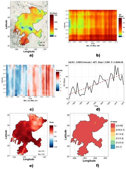
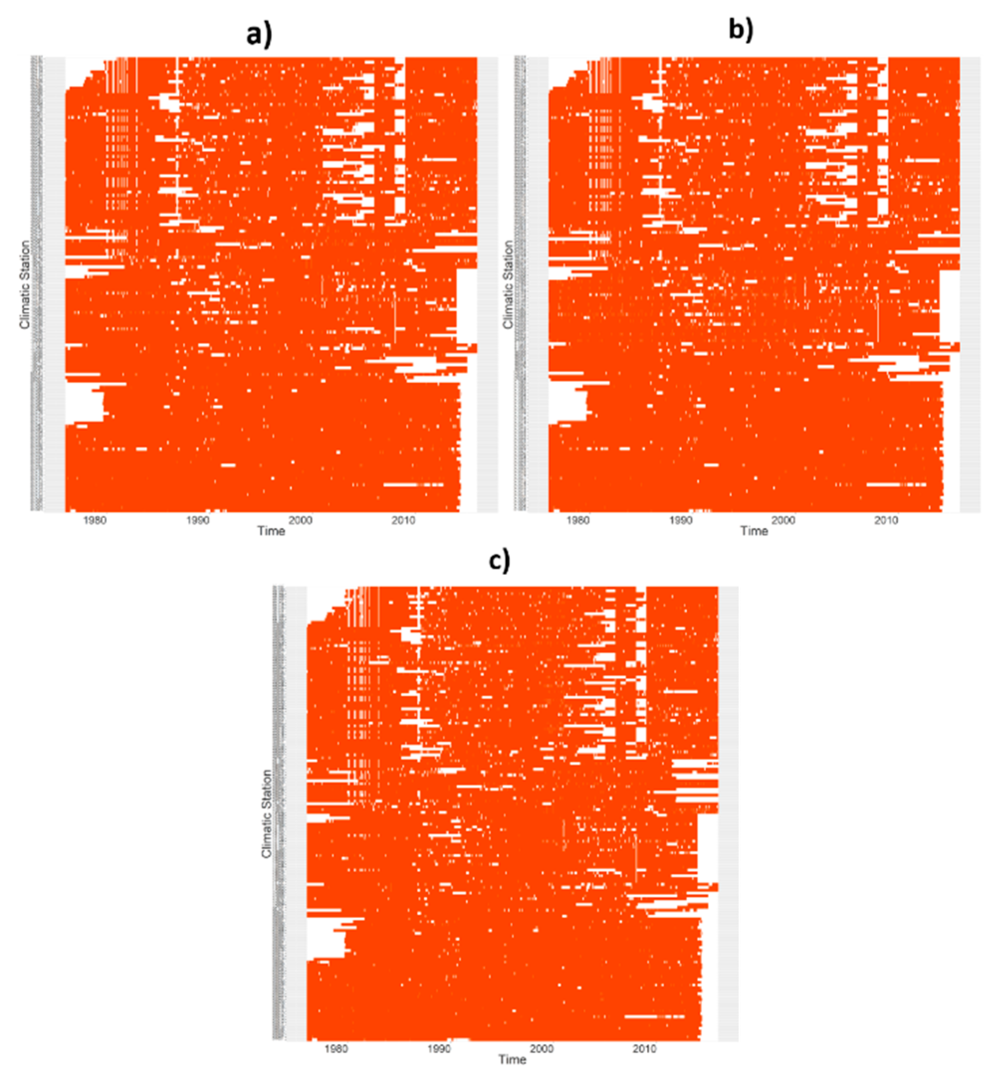
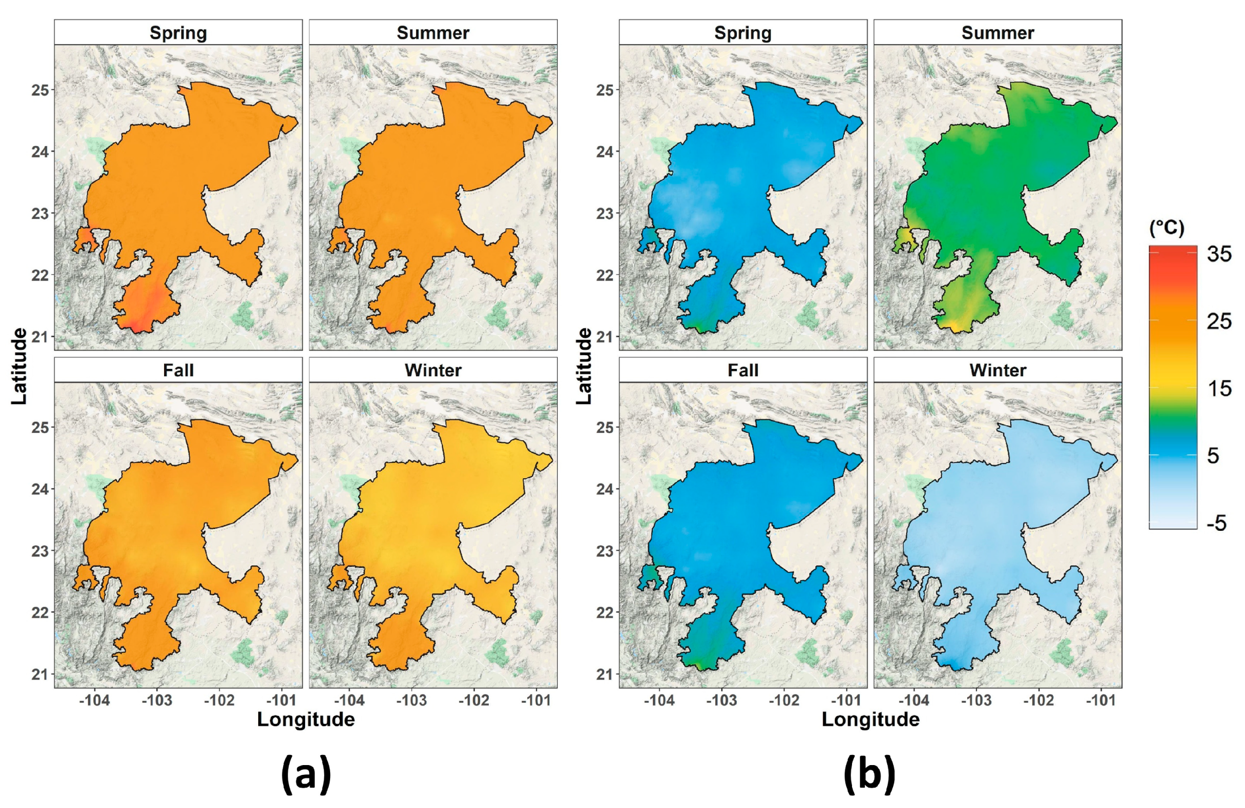
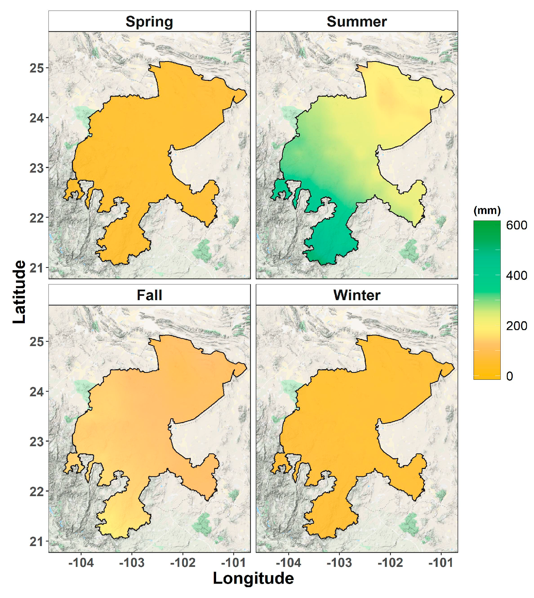
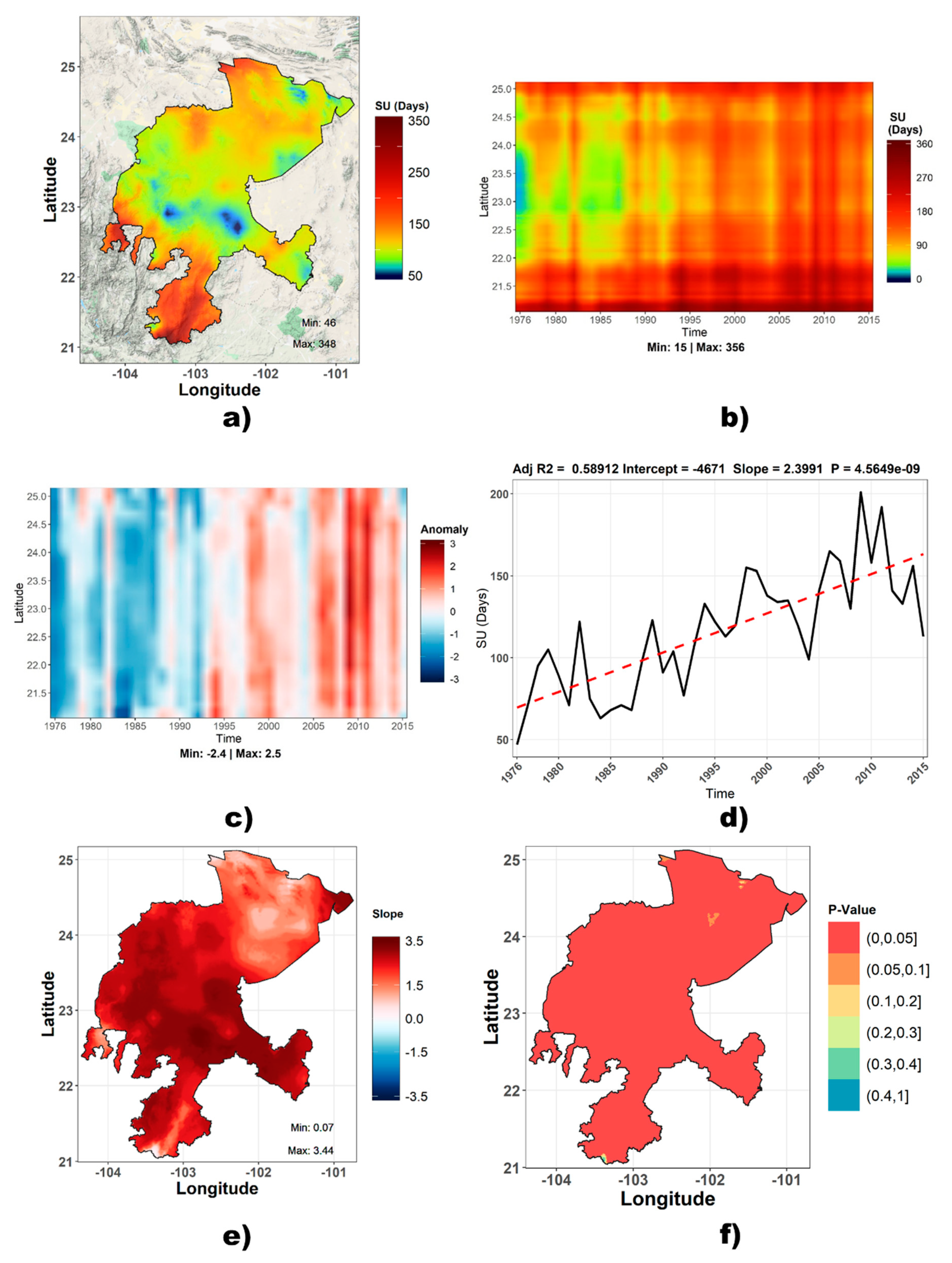
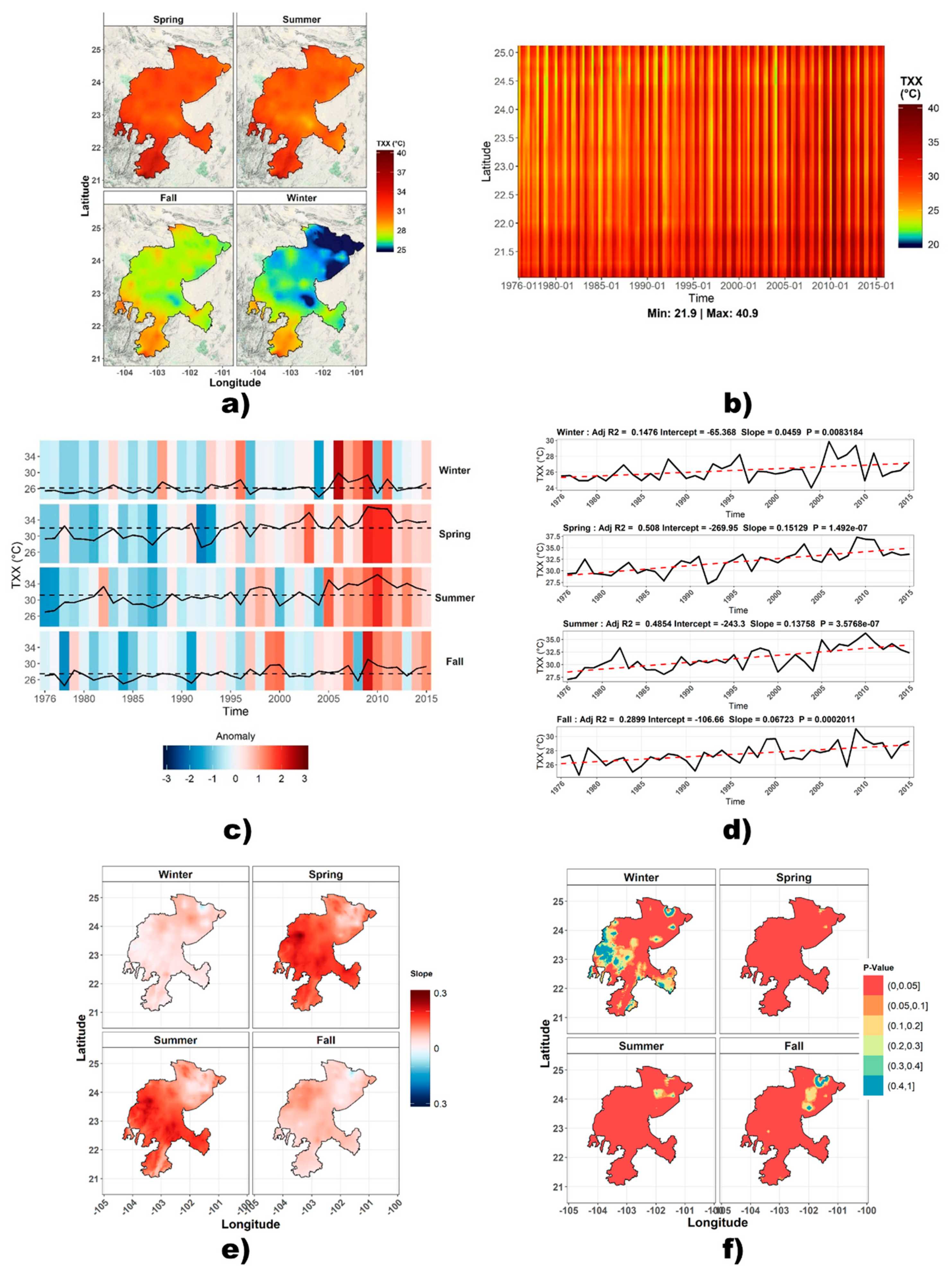
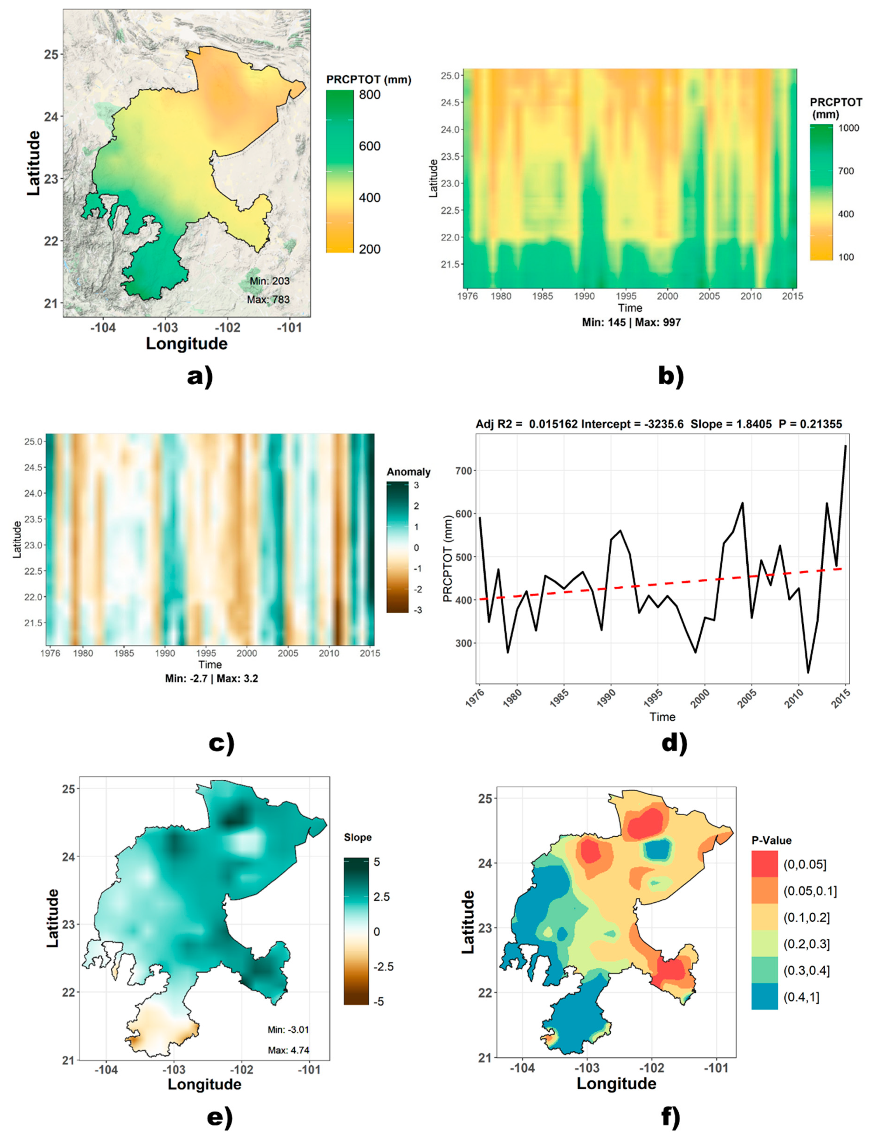
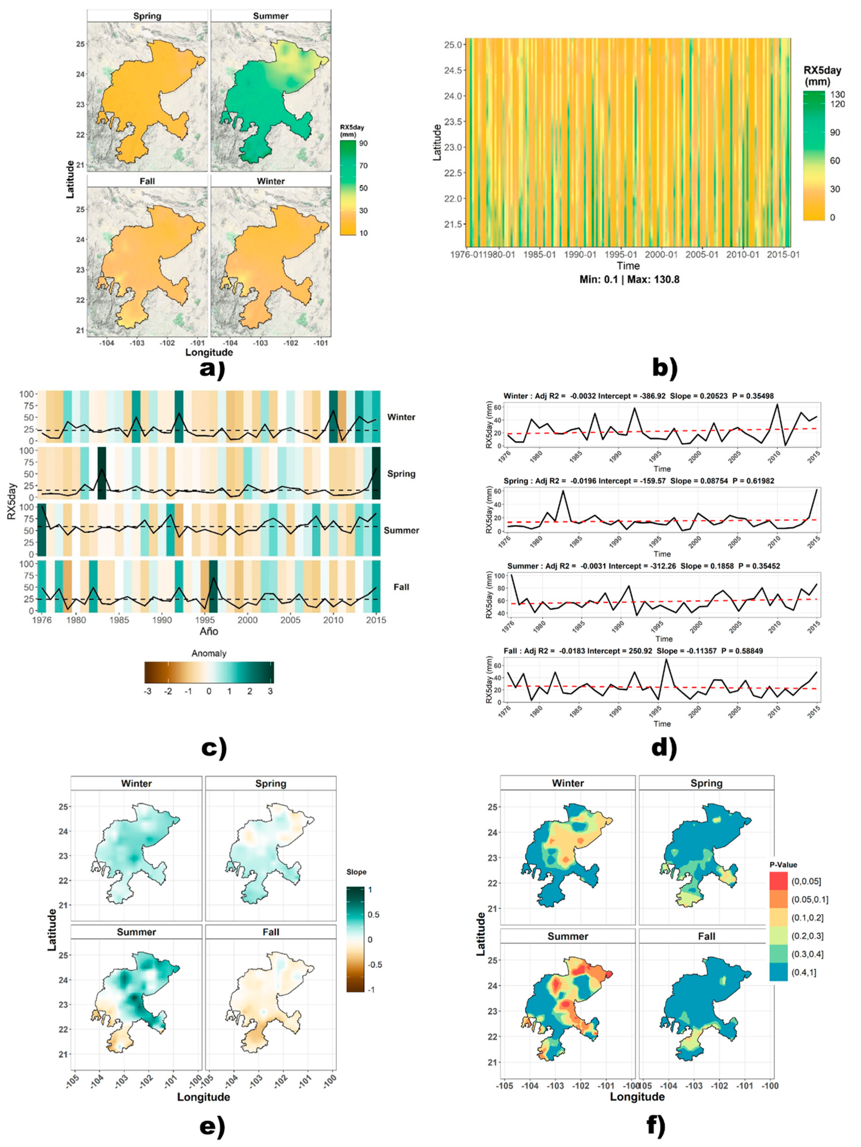
Table 1.
Climate and reanalysis stations used for quality control, homogenization, and data filling in the state of Zacatecas.
Table 1.
Climate and reanalysis stations used for quality control, homogenization, and data filling in the state of Zacatecas.
| Variable | Number of Stations | ||
|---|---|---|---|
| Climatic Stations | Reanalysis Stations | Total | |
| TMAX | 140 | 43 | 183 |
| TMIN | 139 | 40 | 179 |
| PP | 158 | 44 | 202 |
Table 2.
Climate change indices used for analysis in the state of Zacatecas.
| Temperature Indices | Description | Precipitation Indices | Description |
|---|---|---|---|
| SU | Summer days | PRCPTOT | Total precipitation |
| FD | Frost days | CDD | Consecutive dry days |
| TXx | Extreme maximum temperature | Rx1day | Daily maximum precipitation |
| TNn | Extreme minimum temperature | Rx5day | Maximum consecutive 5-day precipitation |
Table 3.
Maximum and minimum seasonal values for maximum and minimum temperatures in the state of Zacatecas.
Table 3.
Maximum and minimum seasonal values for maximum and minimum temperatures in the state of Zacatecas.
| Spring | Summer | Fall | Winter | ||
|---|---|---|---|---|---|
| TMAX | Max | 34.1 | 30.7 | 29.4 | 28.2 |
| Min | 22.2 | 21.3 | 19.4 | 16.0 | |
| TMIN | Max | 12.8 | 17.3 | 13.2 | 7.6 |
| Min | 3.3 | 8.7 | 4.7 | −1.2 |
Table 4.
Maximum and minimum seasonal precipitation values in the state of Zacatecas.
| Spring | Summer | Fall | Winter | ||
|---|---|---|---|---|---|
| PREC | Max | 60.6 | 545.5 | 195.8 | 64.0 |
| Min | 18.6 | 112.3 | 67.4 | 25.5 |
Table 5.
Maximum and minimum seasonal values (°C) of the extreme maximum temperature index in the state of Zacatecas.
Table 5.
Maximum and minimum seasonal values (°C) of the extreme maximum temperature index in the state of Zacatecas.
| Spring | Summer | Fall | Winter | ||
|---|---|---|---|---|---|
| TXx | Max | 39.1 | 38.0 | 33.1 | 33.7 |
| Min | 29.9 | 28.4 | 25.6 | 23.9 |
Table 6.
Maximum and minimum seasonal values (°C) of the extreme minimum temperature index in the state of Zacatecas.
Table 6.
Maximum and minimum seasonal values (°C) of the extreme minimum temperature index in the state of Zacatecas.
| Spring | Summer | Fall | Winter | ||
|---|---|---|---|---|---|
| TNn | Max | 6.0 | 14.1 | 4.9 | 2.4 |
| Min | −5.8 | 3.7 | −6.2 | −9.1 |
Table 7.
Maximum and minimum seasonal values of the daily maximum precipitation index (mm) in the state of Zacatecas.
Table 7.
Maximum and minimum seasonal values of the daily maximum precipitation index (mm) in the state of Zacatecas.
| Spring | Summer | Fall | Winter | ||
|---|---|---|---|---|---|
| Rx1day | Max | 15.8 | 37.9 | 31.2 | 20.4 |
| Min | 5.5 | 12.3 | 11.4 | 8.1 |
Table 8.
Maximum and minimum seasonal values (mm) of the maximum consecutive 5-day precipitation index in the state of Zacatecas.
Table 8.
Maximum and minimum seasonal values (mm) of the maximum consecutive 5-day precipitation index in the state of Zacatecas.
| Spring | Summer | Fall | Winter | ||
|---|---|---|---|---|---|
| Rx5day | Max | 27.2 | 90.6 | 36.2 | 35.6 |
| Min | 10.5 | 32.0 | 15.4 | 15.5 |
© 2020 by the authors. Licensee MDPI, Basel, Switzerland. This article is an open access article distributed under the terms and conditions of the Creative Commons Attribution (CC BY) license (http://creativecommons.org/licenses/by/4.0/).
Share and Cite
MDPI and ACS Style
Pita-Díaz, O.; Ortega-Gaucin, D. Analysis of Anomalies and Trends of Climate Change Indices in Zacatecas, Mexico. Climate 2020, 8, 55. https://0-doi-org.brum.beds.ac.uk/10.3390/cli8040055
AMA Style
Pita-Díaz O, Ortega-Gaucin D. Analysis of Anomalies and Trends of Climate Change Indices in Zacatecas, Mexico. Climate. 2020; 8(4):55. https://0-doi-org.brum.beds.ac.uk/10.3390/cli8040055
Chicago/Turabian StylePita-Díaz, Oscar, and David Ortega-Gaucin. 2020. "Analysis of Anomalies and Trends of Climate Change Indices in Zacatecas, Mexico" Climate 8, no. 4: 55. https://0-doi-org.brum.beds.ac.uk/10.3390/cli8040055
Note that from the first issue of 2016, this journal uses article numbers instead of page numbers. See further details here.