Greening and Browning Trends of Vegetation in India and Their Responses to Climatic and Non-Climatic Drivers


1
Department of Geoinformatics, School of Natural Resource Management, Central University of Jharkhand, Ranchi 835205, India
2
Department of Agriculture & Soil, Indian Institute of Remote Sensing, Indian Space Research Organisation, Department of Space, Government of India, Dehradun 248001, India
*
Author to whom correspondence should be addressed.
Climate 2020, 8(8), 92; https://0-doi-org.brum.beds.ac.uk/10.3390/cli8080092
Submission received: 13 July 2020
/
Revised: 2 August 2020
/
Accepted: 7 August 2020
/
Published: 9 August 2020
Abstract
:It is imperative to know the spatial distribution of vegetation trends in India and its responses to both climatic and non-climatic drivers because many ecoregions are vulnerable to global climate change. Here we employed the NDVI3g satellite data over the span of 35 years (1981/82–2015) to estimate vegetation trends and corresponding climatic variables trends (i.e., precipitation, temperature, solar radiation and soil moisture) by using the Mann–Kendall test (τ) and the Theil–Sen median trend. Analysis was performed separately for the two focal periods—(i) the earlier period (1981/82–2000) and (ii) later period (2000–2015)—because many ecoregions experienced more warming after 2000 than the 1980s and 1990s. Our results revealed that a prominent large-scale greening trend (47% of area) of vegetation continued from the earlier period to the later period (80% of area) across the northwestern Plain and Central India. Despite climatologically drier regions, the stronger greening trend was also evident over croplands which was attributed to moisture-induced greening combined with cooling trends of temperature. However, greening trends of vegetation and croplands diminished (i.e., from 84% to 40% of area in kharif season), especially over the southern peninsula, including the west-central area. Such changes were mostly attributed to warming trends and declined soil moisture trends, a phenomenon known as temperature-induced moisture stress. This effect has an adverse impact on vegetation growth in the Himalayas, Northeast India, the Western Ghats and the southern peninsula, which was further exaggerated by human-induced land-use change. Therefore, it can be concluded that vegetation trend analysis from NDVI3g data provides vital information on two mechanisms (i.e., temperature-induced moisture stress and moisture-induced greening) operating in India. In particular, the temperature-induced moisture stress is alarming, and may be exacerbated in the future under accelerated warming as it may have potential implications on forest and agriculture ecosystems, including societal impacts (e.g., food security, employment, wealth). These findings are very valuable to policymakers and climate change awareness-raising campaigns at the national level.
1. Introduction
The main component of the terrestrial biosphere is vegetation and it plays an active role in the climate system through the exchange of energy, carbon, water and momentum between the biosphere and the atmosphere [1,2]. In recent decades, land use change and climate variability have been affecting the terrestrial biosphere through changing the energy balance [3]. Human-induced land use change and climate variability could have pronounced effects on agricultural production, forestry, natural ecosystems and biodiversity in the future [4]. Commonly, precipitation and temperature are two important climate drivers that affect plant growth and distribution, albeit other climate drivers such as soil moisture, solar radiation, atmospheric CO2 concentrations and nutrients, among others also regulate the vegetative growth. Over the Indian continental regions, average temperatures during the summer monsoon season (June–September) have increased by 0.25 °C since the mid-1990s [5] and are projected to rise by up to 2.8–3.8 °C in the future in response to the build-up greenhouse gases in the atmosphere [6,7].
From a climate point of view, India receives more than 75% of rain during the monsoon (June–September) season. A shift in precipitation pattern can have a profound impact on agriculture, forestry and water resources in India. The vegetation growth pattern and responses are highly dependent on the monsoon-dominant climate over the Indian subcontinent [6,8] and the spatial patterns of precipitation are highly shaped by the peculiar orographic features, such as the Himalayas, the Karakoram and the Hindukush [6]. The southwest monsoon originating from the Bay of Bengal is also a primary source of rainfall over South Asian countries such as Pakistan, Bangladesh, Myanmar, Nepal and Sri Lanka [9]. The seasonal trends of monsoon rainfall in India during the past three decades (1980–2010) have been different over the eastern and western parts of the country. Previous findings suggested that the increasing rainfall trends are more profound west of 80°E, whereas largely negative or decreasing trends are present towards the eastern region [10]. This asymmetry in trends of monsoon rainfall between eastern and western segments is mostly associated with changes in large scale thermodynamic parameters, such as wind speed and moisture content [11].
Vegetation starts growing mainly from the onset of summer monsoon over the Indian subcontinent and within the growing season vegetation greenness is largely influenced by summer monsoon rainfall activities across large parts of the continent. The vegetation growth pattern is commonly used to monitor the productivity of natural forests and agricultural lands, and trends such as “declining or browning” and “increasing or greening” have been commonly used, including assessment of the climate feedback mechanism [12,13,14,15]. These trends are not constantly monotonic but can change from positive to negative trends and vice versa.
Several studies have used the remotely sensed vegetation indices, such as the normalized difference vegetation index (NDVI) and leaf area index (LAI) to determine variations and trends in vegetation growth [13,16,17]. Changes of NDVI trend can be either gradual or abrupt, or more rarely, non-existent [13], and the shift from one to another one can be computed using the breakpoints (change points) in trends [18]. Regardless of changes in NDVI trend spatially and temporally, the critical issue is detecting the changes for understanding the process in the context of broader global change. Commonly, a browning trend (decreasing NDVI) of vegetation greenness is considered to indicate a decrease in the plant growth rate as an indicator of phenological change [19], crop status [20], inter-annual dynamics of vegetation [21], land cover change [22], stress and land degradation [23], temperature-induced drought stress or insect disturbances [24,25], fire activity [26] and ocean circulation anomalies [27]; assessment of vegetation response to climate change should be considered is such cases [28]. In contrast to browning trends, a greening trend (increasing NDVI) of vegetation greenness is interpreted as increase photosynthesis and plant growth and attributed to increasing temperatures [29], earlier spring onset [18,30], lengthening of the growing season [31,32], rainfall or reduced snow cover [33,34], the atmospheric CO2 fertilization effect [35], decreasing cloud cover with associated increases in solar radiation [36], El Nino-Southern Oscillation (ENSO) and the positive phase of the Arctic Oscillation (AO) signal [37]. Thus, the greening trend helps to account for the increase of carbon drawdown in the terrestrial biosphere [38].
Typically, NDVI is used to monitor vegetation growth and is known as a surrogate measurement of plant photosynthetic activity [31]. NDVI is related to structural properties of plants, such as LAI, green biomass, chlorophyll content, foliar nitrogen and productivity [39,40]. The NDVI normalizes green leaf scattering in the near-infrared range and chlorophyll absorption in the red wavelengths. NDVI is a scalable index derived from the near-infrared (0.72–1.0 µm) and red bands (0.58–0.68 µm) and is commonly linked to a variety of vegetation properties and may have multiple explanations for a change in greenness signals. The third generation of the GIMMS NDVI (NDVI3g) data is the only global vegetation record which spans over three decades [41] and allows the quantification and assessment of vegetation changes as a result of changes in ecosystem properties and changes in climate conditions. The most vulnerable ecosystems to climate change are forest and agriculture in South Asia [42] because climate change affects agriculture and food system performance by shifting the spatial and temporal patterns of temperature, rainfall and water availability, land use land cover (LULC), biodiversity and other resources. Climate change and land degradation are particularly important drivers of food insecurity [43,44], and thus, climatic-driven agriculture ecosystems and food security are emerging as pressing issues across the subcontinent.
Agriculture is the most important livelihood activity in the Indian subcontinent region, providing a substantial source of rural income, employment and food. About 50–75 % of the total work force which belongs to low income, poor and vulnerable sections of society are still engaged in various land-based activities [45]. The growth in food grain production and water facilities are not able to meet the population explosion. Furthermore, the dramatic climatic and environmental changes over the Indian subcontinent will change the conditions for food production, and thereby the critical scenario poses many challenges to achieving food security. A key aspect of this challenge is that ongoing and future climate changes are projected to have an adverse effect on agricultural production, especially in the Indian subcontinent where water scarcity is of immense concern [46,47]. Agricultural production is a key indicator for food security and several studies have explored the connection between crop yields, NDVI and food security [48]. Typically, satellite-derived remote sensing indices such as NDVI and LAI are used as indicators of variation in food production [5,17,49]. These studies suggested that mid-to-late season NDVI characterizes crop yields better than seasonal integrations or maximum NDVI values. Thereby, yield and reflectance relationships are typically robust after mid-season or during peak growing season [49]. Moreover, their relationships can be strongest by masking the influence of non-agricultural vegetation’s signals based on LULC classifications derived from satellite data [50,51].
Based on earlier version of satellite vegetation records (1982–2003) derived from Advanced Very High Resolution Radiometer (AVHRR), Jeyaseelan et al. [52] indicated the greening trend of NDVI (based-on annual average of NDVI) attributed to advancement in agricultural practices, especially during the 1980–1990s. However, the greening trend of NDVI started declining after 1998 in most of the meteorological subdivisions in India [52]. It is still unclear how the natural forests and croplands have been responding to climatic and non-climatic drivers in recent decades. Thereby, the overarching objectives of this study were: (1) to analyze the inter-annual and seasonal vegetation trends (i.e., greening and browning) using unprecedented long-term NDVI3g records over the span of 1981/82–2015 with trend analysis carried out separately for two focal periods, the earlier period (1982–2000) and later period (2000–2015), and (2) to relate them with key driving factors (both climatic and non-climatic) and mechanisms leading to changes in forests and agriculture ecosystems in India with special focuses on the Northwestern Plain, Central India, and South Peninsula ecoregions. The analysis was performed by utilizing the unprecedented more than three decades (1981/82–2015) of satellite vegetation records of NDVI3g [15,53], climatic data (i.e., precipitation, temperature, solar radiation, and soil moisture), and historical long-term agriculture statistics (i.e., crop area, production, irrigated area, fertilizer use, among others). Unlike other studies those are mostly based on annual average of NDVI, here we analyzed annual average and the peak growing season of NDVI (July–October as kharif season and January–March as rabi season) because NDVI-yield relationships may be more significant by filtering out leaf-off seasons NDVI noise [49]. Specifically, we emphasized changes of NDVI across the major ecosystems, such as forests, shrublands, savannas and agriculture across 5°N–40°N since these ecosystems are influenced by ongoing climate change and are also subject to water stress during peak growing seasons [7].
2. Materials and Methods
2.1. Study Area and Climatic Characteristics
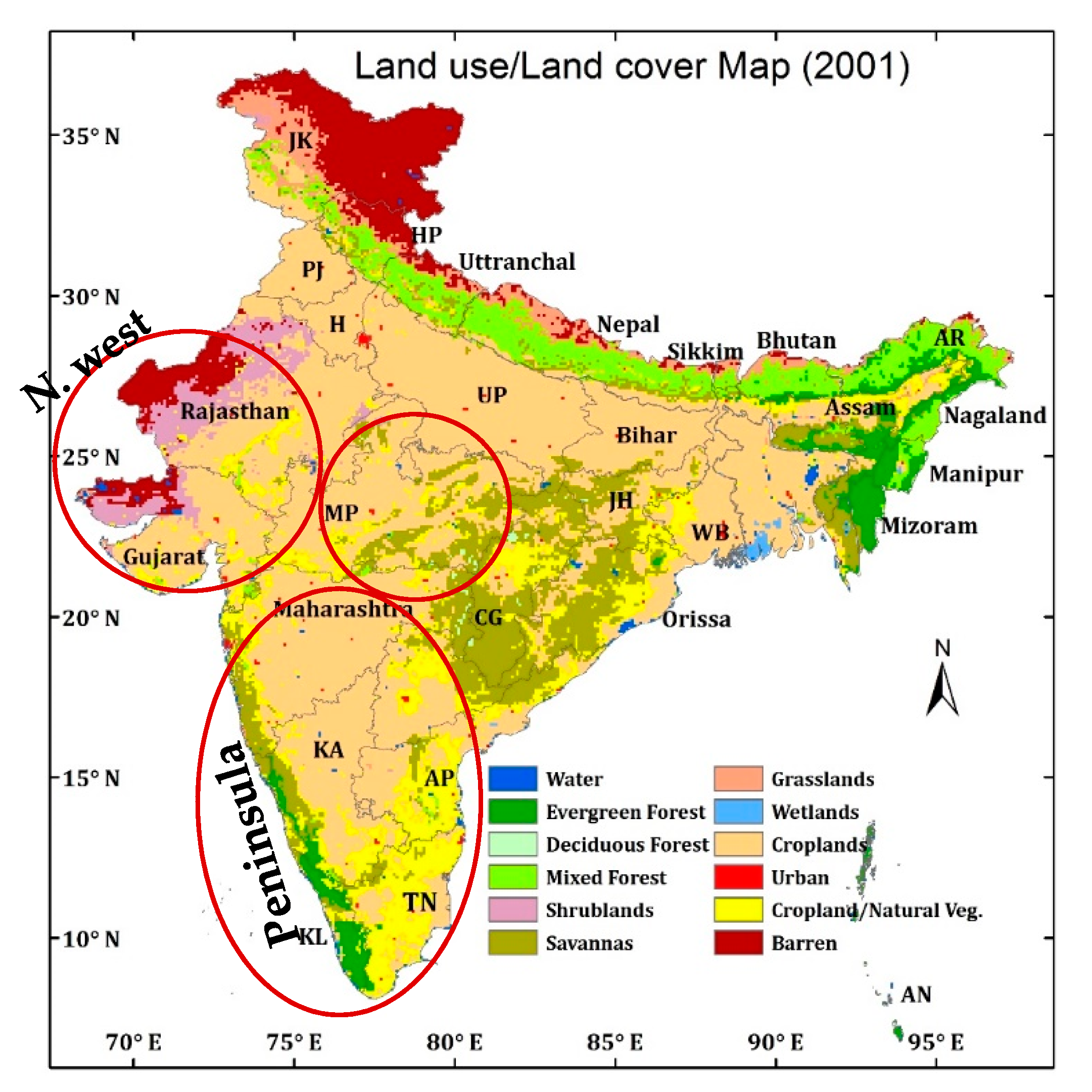
The study area was India which is situated between 8–38°N latitudes and 66–100°E longitudes with a total geographical area of 329 million hectares. As per the Indian Meteorological Department (IMD), India is divided into four broad climatic sub-regions: South Peninsula, Northwest India, Central India, and North and North-East India [54]. These sub-regions are classified into 36 sub-divisions. For this study, we focused mainly on the first three broad climatic sub-regions (i.e., except the North and North-East India). The annual climatic cycle of India is divided into four seasons, namely, (i) pre-monsoon (March to May), (ii) Monsoon (June to September), (iii) post-monsoon (October to December), and (iv) winter (January to February). The monsoon and winter seasons crops are widely known for kharif and rabi seasons, respectively. The South Peninsula comprises Tamil Nadu (TN), Karnataka (KA), Kerala, Andhra Pradesh (AP) and Maharashtra (MH) states; Central India comprises Madhya Pradesh (MP), Chhattisgarh (CG), Jharkhand (JH) and Odisha states; and the Northwestern Plain comprises Rajasthan (RJ) and Gujrat states (Figure 1). These climatic sub-regions include a wide range of variations in topography, LULC type (Figure 1), and climate. Based on Koppen–Geiger climate classification, arid conditions are present in Northwest India; the South Peninsula has tropical, wet and dry climates; and there is a semi-arid climate in Central India. The large spatial variability of south west (SW) summer monsoon is the main cause for diverse vegetation types across the four broad climatic sub-regions. (Figure 1). Forest and agriculture account for nearly 80% of the geographical area of India, about 24.56% of which is forest and 55% of which is agricultural land [55].
2.2. Data Used
In this study, we used time-series satellite data, climate data and various ancillary data, and detailed characteristics are presented in Table 1. Precipitation and temperature are abbreviated as prec and temp.
(1) NDVI3g: We used the improved calibrated and extended long-term satellite vegetation records of NDVI from the Global Inventory Modeling and Mapping Studies (GIMMS). The third generation of the GIMMS NDVI (henceforth, NDVI3g) data builds on its predecessor NDVIg with a native resolution of 0.0833° spanning from 1981 to 2015 and obtained from measurements of NOAA’s AVHRR sensors [53]. These data were aggregated into monthly time steps by taking maximum value compositing (MVC) to eliminate any biases caused by atmospheric conditions [13]. The latest version of NDVI3g data have been calibrated against other NDVI datasets [56] and considered the best dataset for analyzing long-term NDVI trends and characterizing vegetation responses to climate variability [41]. However, NDVI3g data have a limitation in spatial resolution (8 km) on the ground which limits their capability regarding portraying vegetation analysis at a fine resolution. They have limited applicability especially over the snow cover regions due to unrealistic low NDVI values (<0.2) [57]. The peak growing season of NDVI was calculated based on the average monthly NDVI from July to October in each calendar year. The vegetation greenness index NDVI was used as a substitute measurement of chlorophyll, and thus, plant photosynthetic activity detects the presence of growing vegetation [40].
(2) MCD12Q1: The combined (Terra and Aqua) Moderate Resolution Imaging Spectroradiometer (MODIS) Land Cover Type (MCD12Q1, v06) data products are available at yearly intervals (2001–2018). The product is derived using supervised classifications of MODIS reflectance data. The classification scheme adopted from the International Geosphere-Biosphere Programme (IGBP) provides 17 LULC classes.
(3) IMD data: IMD-based climatic data (precipitation and temperature): The Indian Meteorological Department (IMD) rainfall and temperature data were available at the National Data Center (NDC), Pune. The National Climate Centre constructed gridded rainfall data with a spatial resolution of 0.25° on a latitude and longitude grid, and they are interpolated from the 7000 rain-gauge stations. The inverse distance weighted interpolation (IDW) method was employed for interpolating daily rainfall from rain-gauge points to grid points [58]. This is the latest (and a unique) dataset for India developed by IMD and a detailed description and quality control are mentioned in Pai et al. [59,60]. In a nutshell, we have used IMD data from 1982–2015 for analyzing the trend and establishing relationships between vegetation and climate. The IMD data have been widely used in India for various applications comprising intra-seasonal to inter-annual variability of rainfall, climate variability, modelled rainfall validations and hydrological applications, among others [61,62,63].
(4) Downward shortwave at surface (dswrf): The surface downward solar radiation was obtained from the Princeton Global Forcings V2, Princeton University, and the dataset is called SRB PGF v2 (http://hydrology.princeton.edu/data/pgf/v2). The monthly coarse-scale (0.5°) gridded surface downward solar radiation is available at global-scale [64].
(5) CPC soil moisture: The monthly CPC Soil Moisture (V2) data obtained from the Leaky Bucket model at 0.5° resolution for the period from 1948 to 2015 [65]. It consists of a file containing monthly averaged soil moisture water height equivalents (mm). The data are available at https://psl.noaa.gov/data/gridded/data.cpcsoil.html. The model used over 17,000 gauges worldwide to produce soil moisture data, and details of validation of data described in Fan and Dool [65].
(6) Non-climatic data: Historical crop statistics data comprise state-wide foodgrain production, fertilizer usages, crop area and irrigated area during kharif season (June–October, rainy season) and rabi season (November–March) for the period 1981–2015, and these data were obtained from the Ministry of Agriculture, Government of India [66]. Foodgrain production corresponds to the total production of kharif crops, such as cereals (rice, wheat, maize, millet, sorghum, etc.) and pulses (beans, peas and lentils, among others). In addition, we have used rabi season crop productions related to crops such as winter wheat and maize, among others. There are some missing data related to consumption of NPK (Nitrogen, Phosphorous, and Potassium) fertilizer during the 1980s and 1990s.
2.3. Methods
(1) Data processing: All coarse-scale climate data (IMD, SRB, CPC) were downscaled (nearest neighbor) to a common 0.0833°spatial grid on which the spatial trend analyses were performed. For Man–Kendall test and Sen’s slope analysis, we used 35 year (1981–2015) time-series data, and further Student’s t-tests were employed to evaluate statistical significance.
(2) NDVI trends using Man–Kendall test: To study the relationship between NDVI and time, we employed the Man–Kendall test [67] on NDVI time series data from 1981/82 to 2015. The computations were performed with the raster, gimms and kendall packages in R programming software. The monotonous trend calculation was applied on annual/seasonal aggregated NDVI data with NDVI pixel values more than 0.2. The inter-annual NDVI trends over croplands and natural vegetation (forests, shrublands and savannas) were found by taking the average values across pixels for each year over the span of 1982–2015. Furthermore, the intra-seasonal NDVI trends were found by taking the average values across pixels over July–October (kharif season) over the span of 1981–2015 and January–March (rabi season) for each year over the span of 1982–2015. The non-parametric test is based on the rank correlation coefficient (τ, hereinafter referred to as Kendall’s τ). The other procedure called pre-whitening, as described in Yue and Wang [68], has been applied to remove lag-1 autocorrelation from the data. Kendall’s τ pixels with the 90% confidence levels (p < 0.1) were highlighted and used for subsequent analysis.
(3) Climatic variable trends using Sen’s slope: The climate data such as rainfall, temperature, solar radiation and soil moisture were used to compute the linear slope that uses the Theil–Sen approach [69,70]. Theil–Sen slope estimator was formulated by Thiel [70] but modified by Sen [69] and computes the median of the slopes between observation values. The trends of NDVI and climate data were determined separately for the two focal periods, namely, 1981–2000 and 2000–2015 on a pixel basis. The trend of pixels corresponds to urban areas and barren land has been masked so that only vegetation pixels have been analyzed. Two focal periods, namely, 1981/82–2000 and 2000–2015 have been considered in order to see the climate controls on vegetation as the period after 2000 have experienced more warming than the 1980s or 1990s. The trends calculated for the period 1981/82–2000 refer to the “earlier period,” and for the period 2000–2015, “later period.”
(4) Pearson’s correlation analysis: The Pearson’s correlations were also performed between NDVI (July–October) and climatic variables, namely, precipitation, temperature, solar radiation and soil moisture (June–September) over the period 1981–2015 to establish long-term relationships between NDVI and climatic factors. Student’s t-tests were employed to evaluate statistical significance. Pearson’s correlations were computed by extracting data from 14 random sample points over the space (western/Central India and southern peninsula) for each year over the period 1981–2015. In other words, correlation was undertaken using 280 points and 224 points in the earlier period (1981–2000) and later period (2000–2015), respectively.
(5) We regrouped 17 IGBP-based LULC types into two broad categories, forests and agriculture. The evergreen, deciduous and mixed forests, shrublands and savannas were grouped under the forests/vegetation class, whereas croplands were kept under agriculture. We masked water bodies/wetland, built-up, grassland and barren or sparse vegetation cover based on the MODIS land cover data. In the analysis, we incorporated only grid cells with NDVI > 0.1. In the results section, we often use the term “peak summer”; it refers to the periods of July–August and August–September for land areas in the Indian subcontinent.
3. Results
3.1. NDVI Trends for Two Focal Periods (1981/82–2000 and 2000–2015)
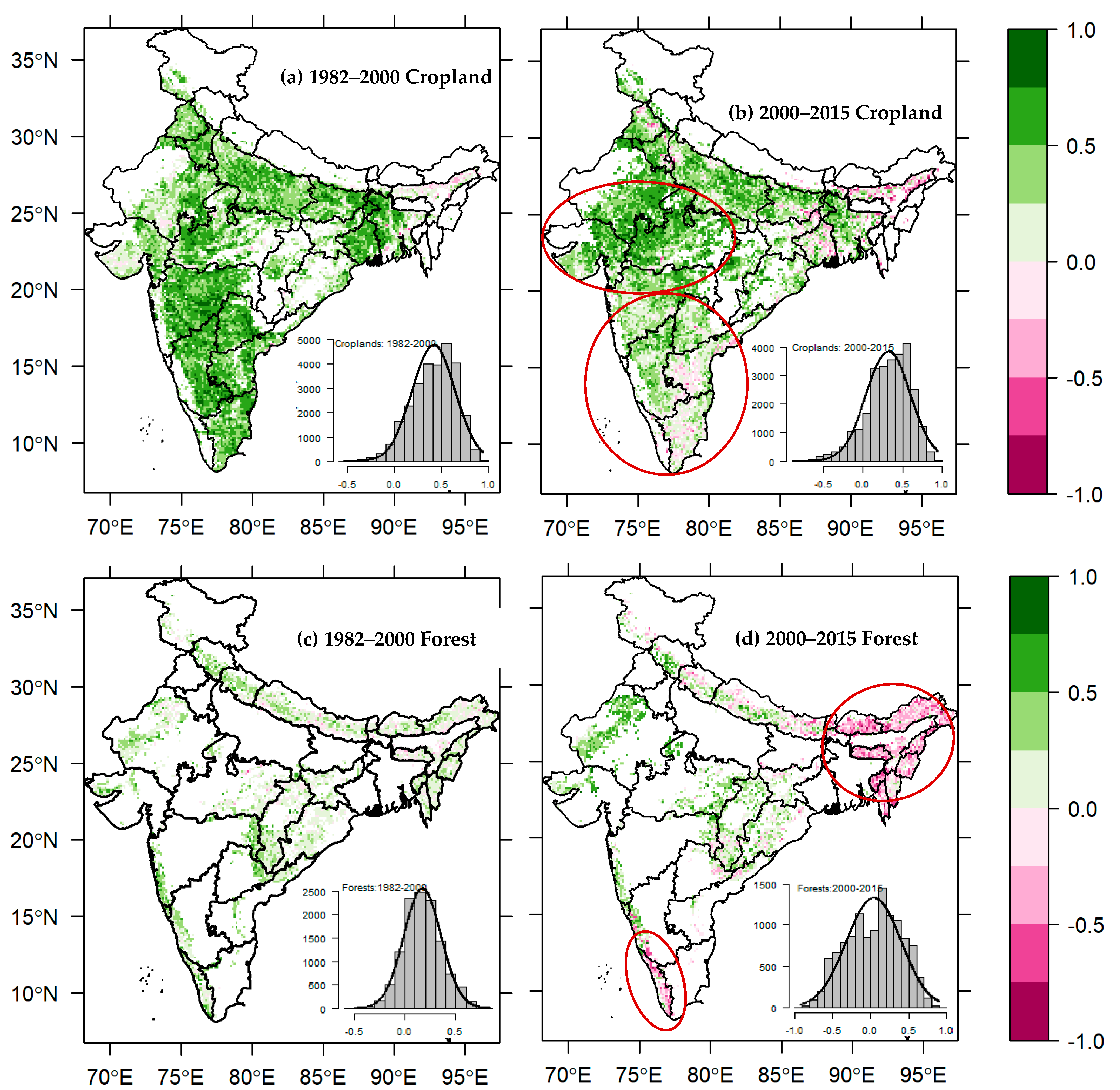
The vegetation greenness index NDVI, known as a surrogate measurement of plant productivity, was analyzed across the Indian subcontinent for the two focal periods separately. The Mann–Kendall NDVI trends (τ) based-on annual mean of NDVI have been illustrated for croplands and forests (including shrublands and savannas) in Figure 2 separately for the earlier period (1982–2000) and the later period (2000–2015) based-on the latest NDVI3g data. In the earlier period (1982–2000), cropland areas exhibited widespread greening trends (Figure 2a). The cropland area under greening trends constituted nearly 81% in the earlier period which diminished to 69% in the later period (Table 2). Compared to the earlier period, greening trends were more pronounced in the later period, especially over the Northwest India (Gujarat and Rajasthan) and Central India (Madhya Pradesh) (Figure 2b). In contrast, the greening trends of the earlier period (Figure 2a) diminished over the South Peninsula in the later period (Figure 2b) leading to no trends or browning trends of croplands. These two contrasting patterns have been highlighted by red color circles in Figure 2b. To understand the greenness/brownness pattern, we gave special attention to these two regions in subsequent analysis. It was also noticed that over the parts of Western Ghats and Northeast India, including the Himalayan regions of the Indian subcontinent, areas of greening trends of forests in the earlier period switched to browning trends in the later period (Figure 2c,d). The forested area under greening trends was nearly 43% in the earlier period and it diminished to 36% in the later period, and the browning trends changed from 0.4% (early period) to 20% (later period) (Table 2).
Moreover, the areas of croplands revealed widespread greening trends when the whole period’s (1982–2015) NDVI (i.e., annual mean) data were used for the Mann–Kendall test (Figure 3a). In contrast, both greening and browning trends were present over forests areas (Figure 3b) when the whole period NDVI was used. Most of the forest areas exhibited greening trends over the Indian subcontinent, whereas some parts of the Western Ghats, the Himalayas, and Northeast India exhibited no significant trend (Figure 3b) and the pattern was quite similar to Figure 2d. The spatial patterns and trends of whole period were consistent with a recent study by Samrah. et al. [16] that demonstrated similar trend patterns using the NDVI3g data over the period 1982–2013 and with Pandey and Ghimire [71], who used relatively less data over the period 1982–2006.
3.2. Inter-Annual NDVI Trends of Forests over the Northwestern Plain, Central India and the South Peninsula
Here we present detailed statistics on greening and browning trends of forest areas, especially over the Northwestern Plain, Central India, and the South Peninsula which are marked by red circles in Figure 2c,d. In the earlier period (Figure 2c), in nearly 47% of areas, forests had greening trends and these greening trends continued and increased up to 80% in the later period over the Northwestern Plain and Central India (Table 3). The areas of greening trends constituted nearly 71% over the South Peninsula and western peninsula in the early period but significantly reduced to 34.5% in the later period (Figure 2d and Table 3), and this was because of more forest areas under browning trends in the Western Ghats of India, as displayed by red circles in Figure 2d.
3.3. Inter-Annual and Intra-Seasonal NDVI Trends of Croplands over the Northwestern Plain, Central India and the South Peninsula
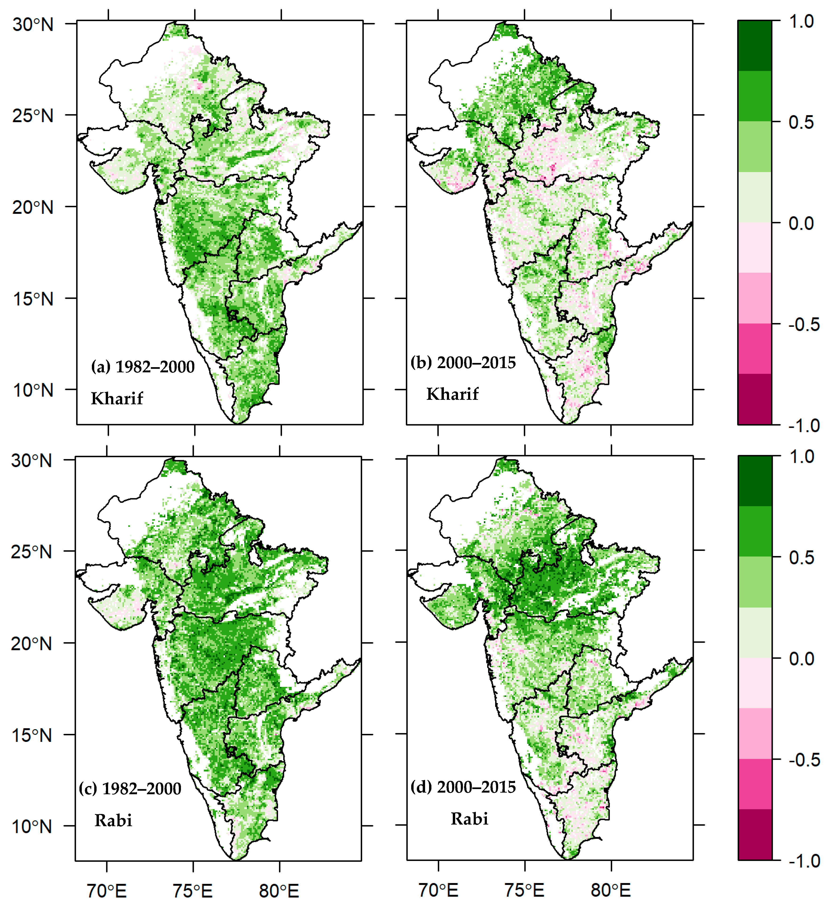
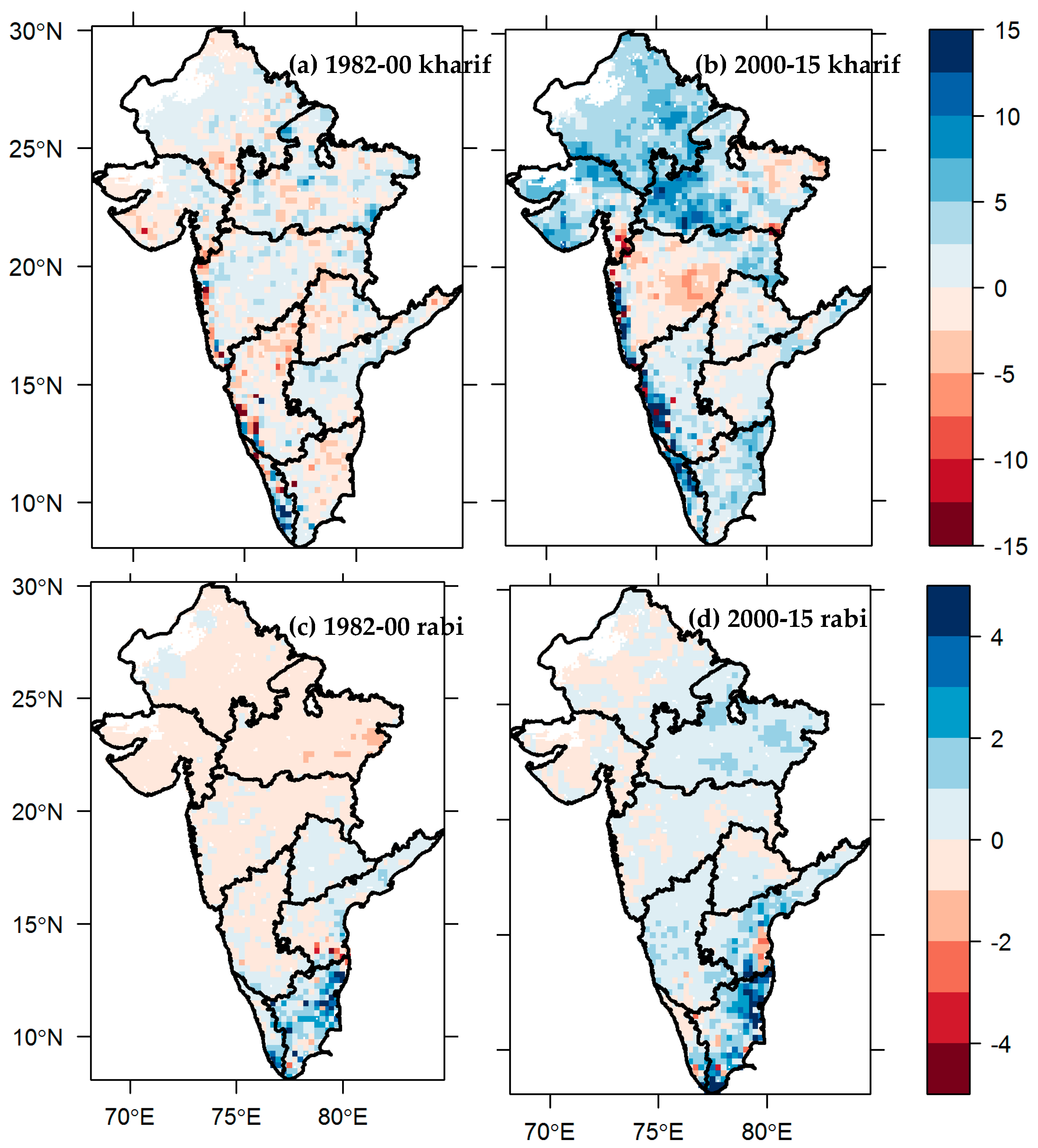
The intra-seasonal NDVI trends of croplands in kharif and rabi seasons revealed widespread diminishing patterns of greening trends of NDVI in the later period compared to earlier period (Figure 4). In other words, the browning trends during kharif season were significantly increased in the later period, especially over Central India (MP) and the Southern Peninsula (i.e., Kerala, TN, AP, TL, KA and MH) (Figure 4a,b). Conversely, the growth of croplands improved over Gujarat and Rajasthan, which exhibited increasing greening trends in the later period. In the case of rabi season, there were not many changes of greening trends of croplands from the early period to the later period (Figure 4c,d) over the Northwestern Plain and Central India. In contrast, greening trends diminished over the South Peninsula and the western peninsula (MH) in the later period compared to the earlier period (Figure 4c,d). This indicates that the agriculture growth pattern stagnated or declined profoundly over the South Peninsula and the western peninsula (MH), but it improved over the Northwestern Plain both in kharif and rabi seasons.
The percentage areas under three categories, namely, browning trend, no trend and greening trend, are presented in Table 4. The results indicate that areas with greening trends in the kharif season during earlier period constituted 54%, which was marginally increased to about 57% during the later period in the Northwestern Plain and Central India. Conversely, cropland areas of greening trends significantly diminished over the South Peninsula and western peninsula. It was estimated that greening trends of nearly 84% of areas in the earlier period reduced to 40% in the later period because most of the areas of greening trends switched to no trends or browning trends (Table 4). In the rabi season, greening trends continued to the later period (i.e., from 84 to 89%) in the Northwestern Plain and Central India. In contrast, areas of greening trends of croplands substantially decreased from the earlier period (87.9%) to later period (57.9%) (Table 4) as most of the areas of greening trends switched to either no trends or browning trends.
3.4. Inter-Annual Climatic Variable Trends over the Northwestern Plain, Central India and the South Peninsula
In order to understand the climate controls on such large-scale changes in greening trends from the earlier period to the later period, we investigated climate controlling factors, such as precipitation, temperature, soil moisture and solar radiation. Figure 5 illustrates Sen’s slopes for the rainfall (a, b) and temperature (c, d) based on the IMD data. In the earlier period (Figure 5a), most areas displayed either decreasing trends or no trends of rainfall. However, the decreasing trend changed to a large-scale increasing trend (i.e., >2 mm/year) of rainfall in the later period over the Northwestern Plain and Central India (Figure 5b). The corresponding percentage area of increasing trend of rainfall was nearly 24% in the earlier period, whereas it increased to 85% in the later period (Table 5). In the South Peninsula and western peninsula, nearly 59% of areas displayed either decreasing trends or no trends of rainfall in the earlier period, whereas about 41% areas (2 to 8 mm/year) depicted increased trends. In the later period, the increasing trend of rainfall was about 51% (Figure 5b; Table 5).
Figure 5c,d represents spatial pattern temperature trends for the two focal periods. In the Northwestern Plain and Central India; the results showed that increasing temperature trended up by 0.5 °C/decade during the earlier period. Notably, this increased/warming trend of temperature shifted to decreasing/cooling trend (i.e., up to 0.5 °C/decade) for the later period. The area under the decreasing or no trend of temperature in the later period over for the Northwestern Plain and Central India was up to 88% (Table 5). In the South Peninsula, both increasing and decreasing trends of temperature up to 0.5 °C/decade were observed during the earlier period. In other words, there were both warming (17%) and cooling (34%) trends. Notably, in the later period, not many areas depicted cooling trends (3.8%), so nearly 96% of areas observed either no trends or warming trends up to 0.5 °C/decade (Figure 5 c,d; Table 5).
With reference to incoming solar radiation over the Northwestern Plain and Central India (Figure 6a,b), it was observed that there was a continuous decreasing trend from the earlier period to the later period (43 to 89%). The soil moisture trends (Figure 6c,d), indicated that there was a continuous increasing trend from the earlier period to the later period (43 to 98%) which was quite similar to precipitation trends. In the South Peninsula (Figure 6a,b), there were increasing trends (80%) of incoming solar radiation in the earlier period, but they switched to decreasing trends in the later period (76%). The soil moisture trends (Figure 6c,d), indicated that there was an increasing trend (76%) in the earlier period, which switched towards relatively decreasing trends in the later period (20%)—which is quite a similar pattern to that of precipitation trends.
3.5. Relation between NDVI and Climatic Variable Trends for Two Focal Periods over Forest and Cropland
From a more quantitative perspective (Table 2–4), a considerably larger number of “significant” greening trends of forests became apparent from the earlier period (i.e., 47% of area) to the later period (i.e., 80% of area) in the Northwestern Plain and Central India. The greening of vegetation can be explained by increased rainfall/soil moisture with decreased temperature trends over these regions. Among these climatic controls, precipitation/soil moisture may have played a greater role, as these regions were characterized by drier (western states) or subtropical (MP) climates. As this region is water-limited, incoming solar radiation has no control over forest growth. There could be other non-climatic controls on such large-scale greening in forest growth, which has been shown in Section 3.7.
In the South Peninsula, there was a large-scale shift of forest growth pattern from greening in the earlier period toward no trend and even to some extent browning in the later period. A considerably larger number of “significant” greening trends of forest growth pattern (i.e., 71% of area) switched to either no trends or browning trends in the later period (i.e., 66% of area) (Table 3). Such a large-scale shift of vegetation growth can be explained by increased temperature trends and concurrently decreasing precipitation/soil moisture trends over these regions. Among these climatic controls, apparently temperature played a greater role on such large-scale shifts. In addition to temperature controls, there may be other non-climatic controls acting on such large-scale changes in forest growth pattern, which has been discussed in Section 3.7.
There were not many changes in both kharif and rabi season’s croplands trends in the later period (Figure 2c,d) compared to earlier periods over the Northwestern Plain (Gujarat and Rajasthan) and Central India (MP). There were some croplands’ trends enhanced by 2–4% from the earlier to later periods. These could be associated with increasing rainfall trends in the later period (Figure 5a,b; Figure A1a,b in Appendix A). Notably, there was a negative/cooling trend of rabi season temperature (0.25 to 1 °C/decade) across the Northwestern Plain and Central India (Figure 5c,d; Figure A2c,d), which in fact benefitted the continued vegetation growth patterns.
In the South Peninsula and the western peninsula (Maharashtra, MH), the intra-seasonal (kharif and rabi season) NDVI trends revealed that the growth of croplands in the kharif season was diminished by displaying either large-scale absence of trends or partial browning trends in the later period (Figure 2a,b). These patterns are mostly attributed to decreasing rainfall trends in the later period (Figure 5a,b; Figure A1a,b) with large-scale warming trends (up to 0.8 °C/decade) of temperature (Figure 5c,d; Figure A2c,d). In the rabi season, there was also a diminished cropland growth pattern in the later period (Figure 2c,d) over the South Peninsula. However, its intensity was much lower than for the cropland trends of the kharif season. These could be associated with relatively increasing rainfall trends in the later period in peninsula India (Figure A1 c,d). It was also noticed that there were both negative/cooling trends (in western peninsula) and positive/warming trends (eastern coast of peninsula) of rabi season temperature (0.5 °C/decade) in the later period (Figure A2c,d), which can be linked to reduced croplands growth patterns.
3.6. Pearson’s Correlation between NDVI and Climatic Variables for Two Focal Periods
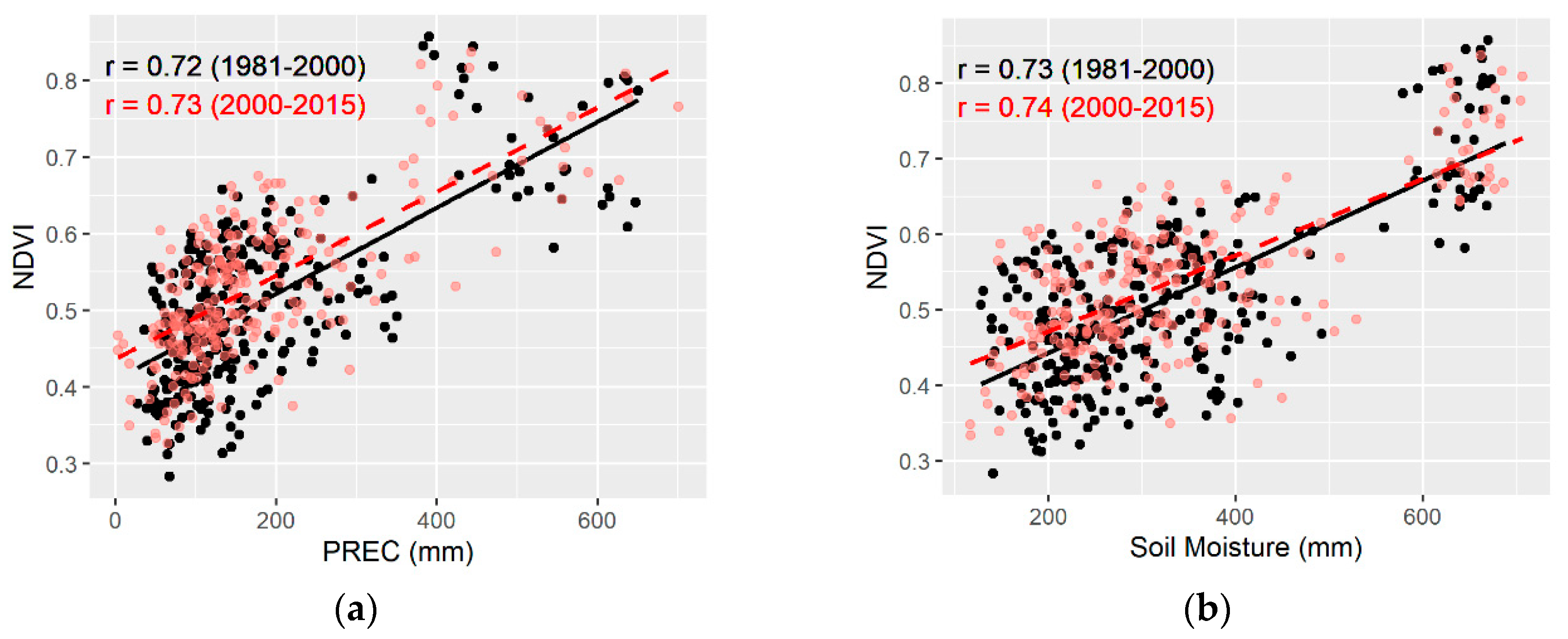
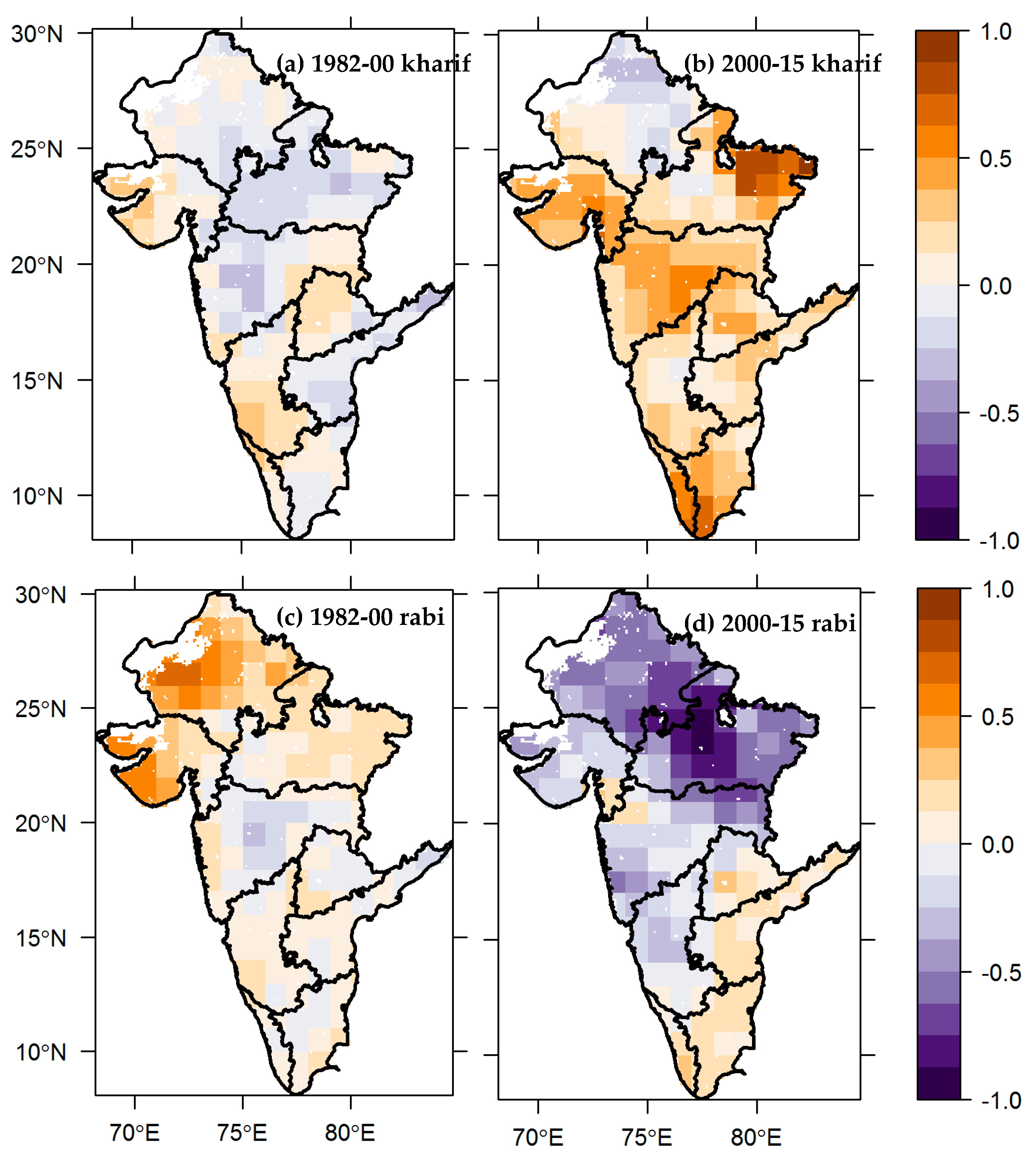
The climatic variables and their control on vegetation growth (as expressed by NDVI) as represented by Pearson’s correlation coefficient (r) are shown in Figure 7. These results showed that precipitation and soil moisture primarily regulated the growth of vegetation (both forests and croplands) in the Northwestern Plain and Central India. There was a positive relationship between the NDVI and precipitation/soil moisture with r ranging from 0.72 to 0.83 (p < 0.001) for both earlier and later periods. However, as these regions are not energy-limited, a negative correlation coefficient was observed between NDVI and solar radiation/temperature with an r value ranging from 0.71 to 0.82 (p < 0.001) for both earlier period and later periods.
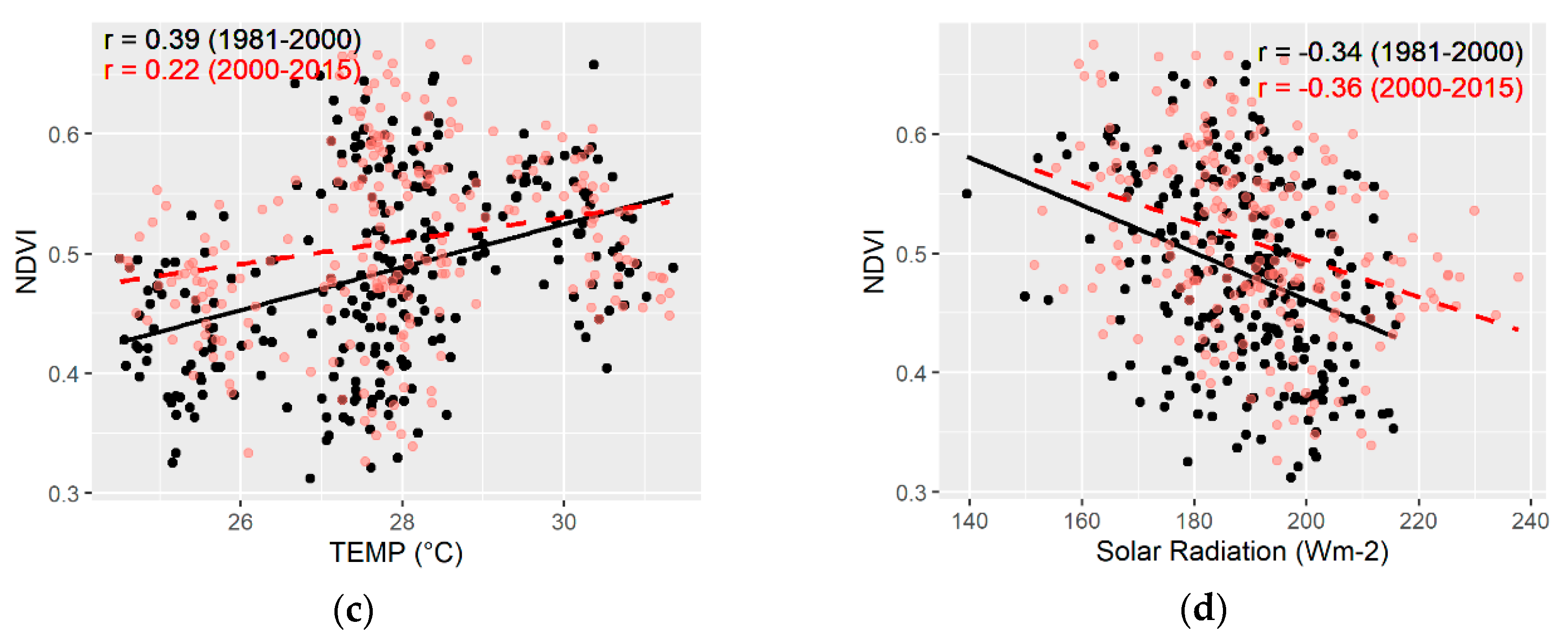
The South Peninsula and the western peninsula regions are also water-limited, including the Western Ghats, and thereby both precipitation and soil moisture are positively correlated with NDVI (Figure 8), which is indicative of both climatic variables playing critical roles in regulating the growth of vegetation. In contrast, there was a weaker positive correlation (r = 0.22–0.39) between NDVI and temperature, indicative of temperature not being the main climatic variable over peninsula India. Over the non-energy-limited peninsula of India, a weak negative correlation (r = 0.34–0.36) between NDVI and solar radiation was noticed, indicative of solar radiation also not being the main climatic variable.
3.7. Relation between Cropland’s NDVI and Non-Climatic Factors in the Northwestern Plain and Central India
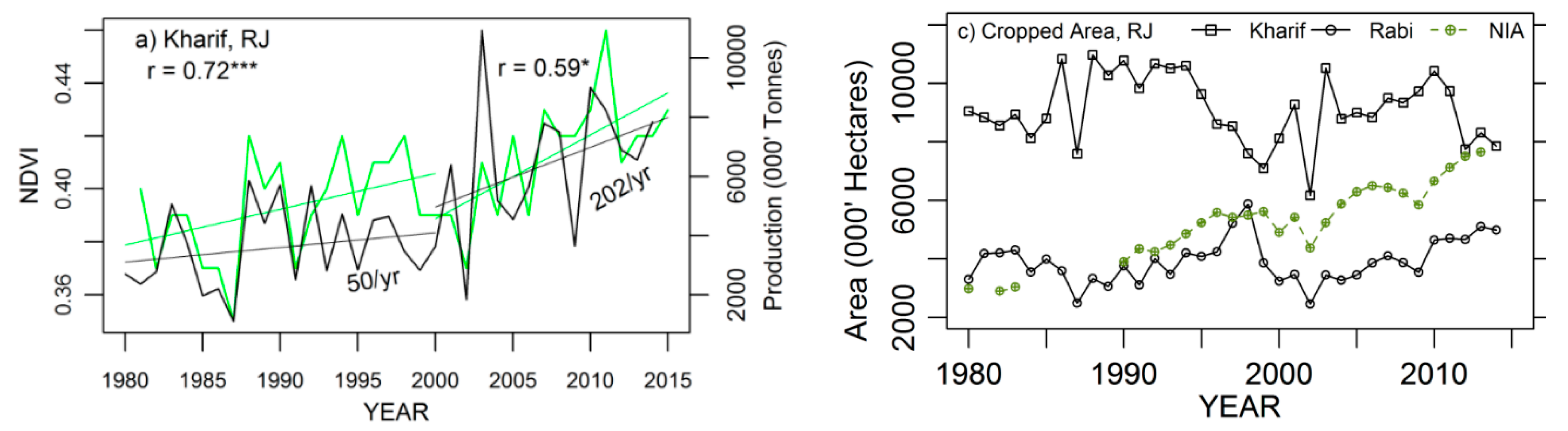
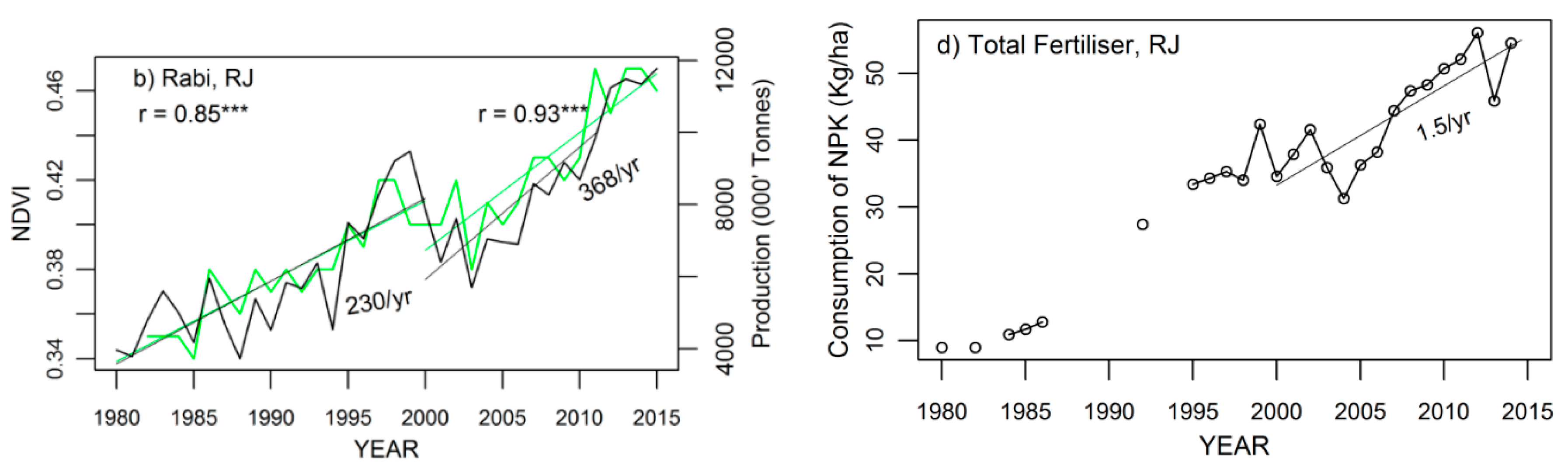
In this section, we address the roles of non-climatic factors, such as changes in cropped area (kharif and rabi), production, area under irrigation and consumption of NPK fertilizers in Rajasthan (RJ) and Madhya Pradesh (MP) states located in the Northwestern Plain and Central India, respectively. In the case of Rajasthan state (Figure 9), the NDVI and kharif season’s foodgrain productions are positively correlated well in both the earlier (Pearson’s r = 0.72) and later periods (Pearson’s r = 0.59), given foodgrain production of 50 thousand tonnes/year in the earlier period and 202 thousand tonnes/year in the later period (Figure 9a). Whereas there was a stronger correlation between the NDVI and rabi season’s foodgrain productions with Pearson’s r > 0.85 (Figure 9b), given foodgrain production of 230 thousand tonnes/year in the earlier period and 368 thousand tonnes/year in the later period (Figure 9b). This increased trends in foodgrain production both in kharif and rabi season were driven by technological changes, such as improved seeds, varieties, fertilizers and mechanization usages, and increased government subsidies. The improved foodgrain production in the later period was well corroborated with the increasing trends of vegetation growth over the Northwestern Plain and Central India. These improved foodgrain production trends were also attributed to the increasing trends of cropping area, net irrigation area (NIA) and consumption of NPK fertilizers in the later period (Figure 9c,d; Table A1).
In the case of MP state (Figure 10), the NDVI and floodgrains productions positively correlated but relatively weaker in kharif season but stronger in rabi season. There was a significant increase in trends of cropping area of rabi, NIA and usages of consumption of NPK fertilizers in the later period (Table A1) which was linked to the continued greening trends over MP. It can be noted that in the year 2000, there was sudden change in the cropping area and foodgrain production which is related to bifurcation of MP state into Chhattisgarh.
3.8. Relation between Cropland’s NDVI and Non-Climatic Factors in the South Peninsula
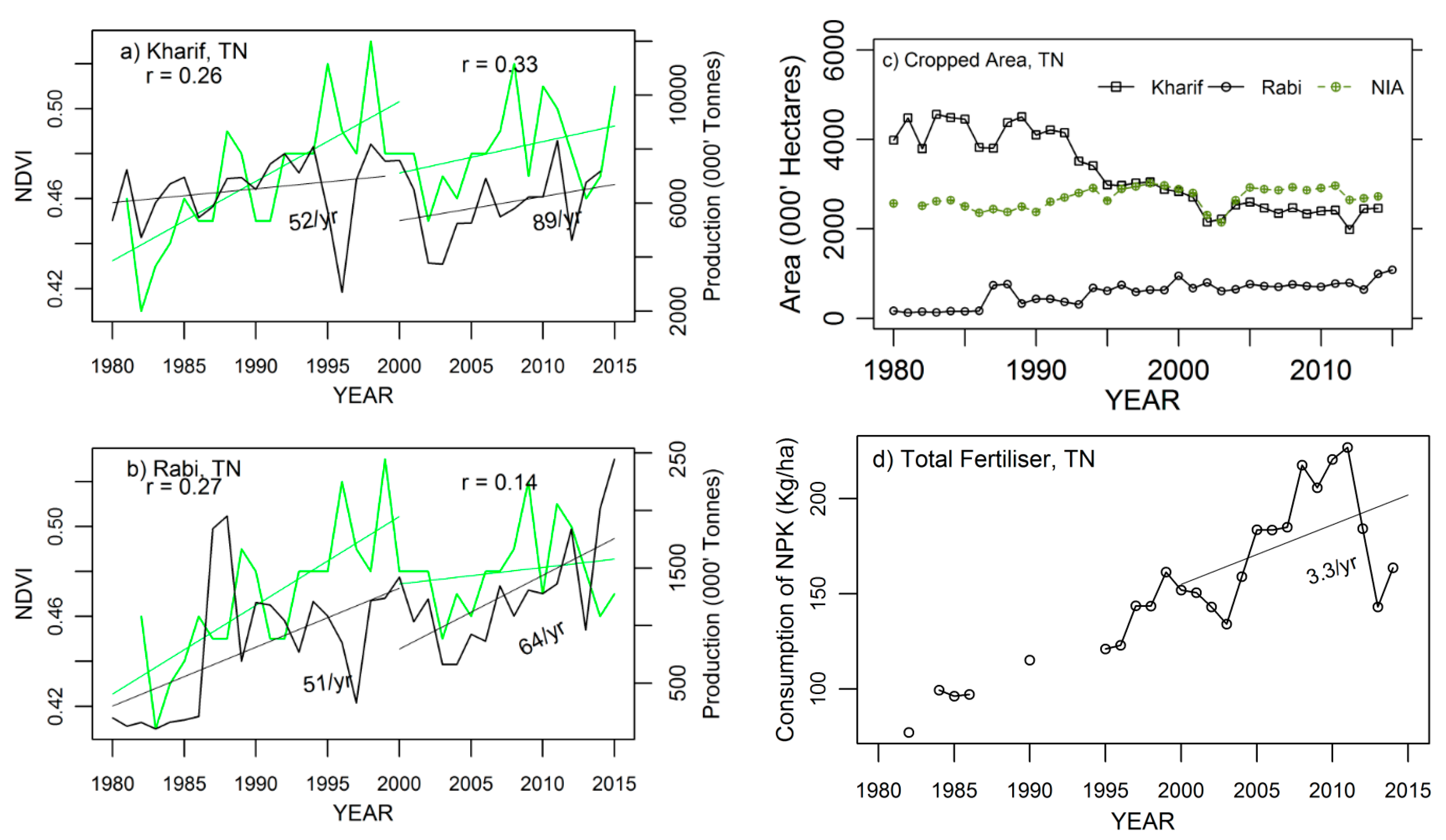
Here, we addressed the roles of non-climatic factors in Tamil Nadu and Andhra Pradesh (AP) states located in the South Peninsula. In the case of Tamil Nadu state (Figure 11), NDVI and kharif/rabi seasons’ foodgrain productions are positively but weakly correlated both in the earlier and the later period. Trends of foodgrain production were 52 thousand tonnes/year in the earlier period and 89 thousand tonnes/year in the later period in kharif season (Figure 11a), whereas in rabi season, the foodgrain production trend was 51 thousand tonnes/year in the earlier period and 64 thousand tonnes/year in the later period. The weaker trend of NDVI in the later period was also associated with land use changes, as depicted in Table A1; areas used in kharif and rabi seasons were dropped substantially and there was a moderate increase in area under NIA (Figure 11c,d). Moreover, it was noticed in Figure 4b,d that there was a large-scale absence of trends and there were large-scale browning trends of vegetation growth in both the seasons.
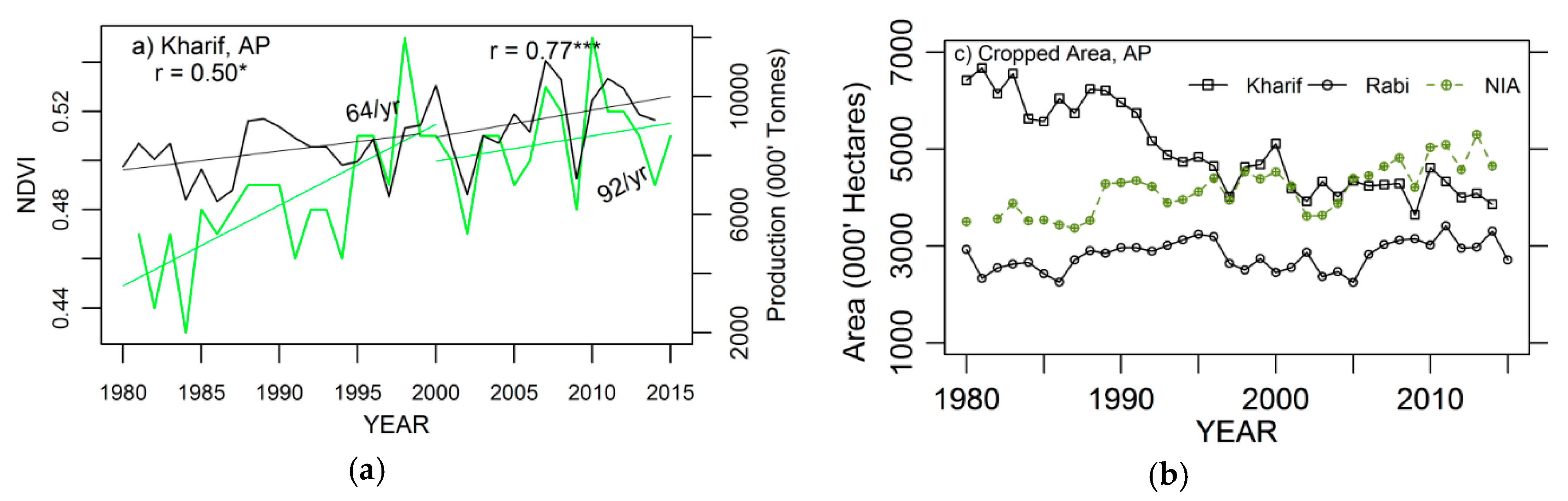
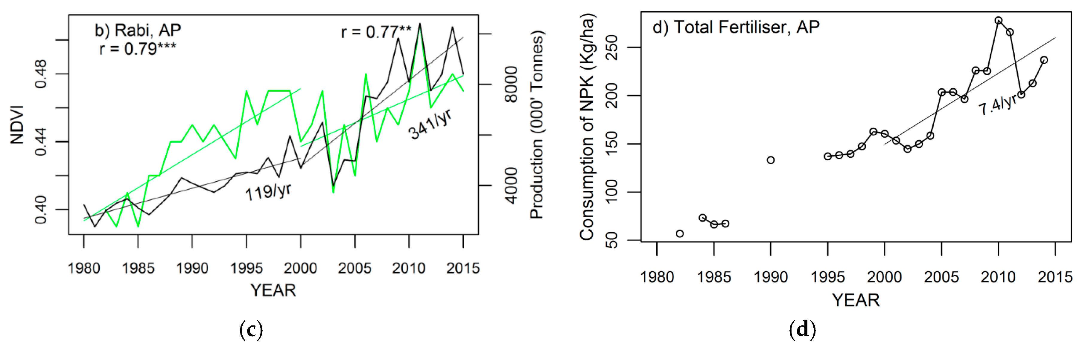
In the case of Andhra Pradesh (AP) state (Figure 12), NDVI and kharif/rabi seasons’ foodgrain productions are positively and strongly correlated both in earlier and later periods (Figure 12a,b). Trends of foodgrain production were 64 thousand tonnes/year in the earlier period and 92 thousand tonnes/year in the later period in kharif season (Figure 12a), whereas in Rabi season, foodgrain production trends were 119 thousand tonnes/year in the earlier period and 341 thousand tonnes/year in the later period. It was noticed that the trends of area under kharif were reduced for both the periods (Figure 12c), both of which were also associated with diminished crop growth, indicating no trends or browning trends (Figure 4b). There were increasing trends of NIA and consumption of NPK (Figure 12c,d).
4. Discussion
This study utilized satellite-derived NDVI time-series (1981/82–2015) data to characterize inter-annual and seasonal trends in vegetation (i.e., forests, woodlands, shrublands) and croplands over India to understand the both climatic and non-climatic drivers behind the observed changes. Both Mann–Kendall and Sen’s slope regression techniques were performed for every pixel to acquire the spatial patterns of linear trends of NDVI and climatic variables, and furthermore, correlation was computed among NDVI and climatic variables. Plants in the Northwestern Plain, Central India, and the South Peninsula are generally sensitive to climatic warming and the biomes, including croplands, were typically water-limited and not temperature-limited. Notably, in the more recent years (2000–2015), temperature increases (up to 1.0 °C/decade) were observed over these regions with pronounced warming in kharif season, In contrast, pronounced cooling trends of temperature (up to –1.0 °C/decade) were seen in the Rabi season. The warming trends in kharif season led to reductions in crop growth, which caused no trends or even browning trends in some parts of Central India, and the South Peninsula. The diminished crop growth pattern was stronger in the South Peninsula than in the Northwestern Plain and Central India. These outcomes are also consistent with some earlier studies that reported declined crop growth from the rabi and kharif seasons’ crops and mostly over the majorly water-limited foodgrain-producing states of India that show resilience for water shortage [5,14]. Moreover, some parts of the Northwestern Plain and Central India (MP) displayed a continued greening trend in the later period (2000–2015), which can be associated with increasing trends of precipitation and soil moisture, a phenomenon known as moisture-induced greening. Furthermore, anthropogenic practices such as technology gains (new crop varieties and hybrids), expansion of irrigation facilities and increased access to surface waters have also supported the continued greening trends of croplands (Table A1; Figure 9c). A significant increase in kharif and rabi season foodgrain production was observed in Central India (Madhya Pradesh) owing to increasing trends of cropping and irrigated area with access to surface waters from the Gandhi Sagar Dam in the Chambal river. These findings are in line with the earlier studies which concluded kharif season growth enhanced over MP in the Chambal valley [5]. It was also observed that there was an increased trend in consumption of fertilizers (3.8 kg/ha in a year) and has a positive relationship with crop growth.
In the case of the South Peninsula, the greening trends of the earlier period during kharif season switched to large-scale absences of trends or browning trends in some parts of peninsula, which can be explained by warming trends of temperature and decreasing trends of precipitation and soil moisture, a phenomenon known as temperature-induced moisture stress [72,73], combined with human-induced LULC changes with clearance of natural vegetation for expansion of urban infrastructures. In rabi season, cooling trends of temperature and also increasing trends of precipitation/soil moisture were attributed to an increase in crop growth, especially over the Northwestern Plain and Central India. However, especially over the South Peninsula, the cooling trends of temperature was not beneficial for crop growth due to water limitation (i.e., negative trend of precipitation/soil moisture). In general, it was observed that greening trends were either sustained or even increased during the rabi season over the kharif season. It can be inferred that the winter season climatic factors contributed greater variability to the vegetation greenness in the Northwestern Plain, Central India and the South Peninsula. These observations are quite similar to those of Sarmah et al. [16], who concluded that higher positive slopes or greening are persistent during the winter season.
Most of the earlier studies related to greening and browning trends have analyzed NDVI data over the Northern parts of India and South Asia by using either the 1982–2005 period, or in some cases 2001–2017 using either NDVI3g data or MODIS-based NDVI and LAI data [16,17,71,74,75,76]. None of the studies have analyzed NDVI trends of vegetation by using long-term time series vegetation data (1981–2015) separately before and after 2000 in response to climatic variables over the climatic sub-regions, such as the South Peninsula, Northwest India, Central India, and North and North-East India. Thus, in the present study, NDVI and climatic trends statistics were presented for the Indian subcontinent and for India’s aforementioned climatic sub-regions. The key findings revealed that nearly 88% of the greening trend was from croplands when whole-period NDVI data were employed (1982–2015) for the Indian subcontinent, and forests accounted for nearly 56% of greening trends. A recent study by [17] analyzed the whole of India using MODIS-based LAI records over the span of 2001–2017 and concluded that the greening is mainly from croplands (82%) with minor contributions from forests (4.4%) in India. In contrast, Chakraborty et al. [74] indicated 12% browning trends and 67% greening trends in natural vegetation (mostly forests and woody trees) in India by using MODIS NDVI data over the span of 2001–2014 [17]. Our results depicted that vegetation over Northeast India and Himalayas had a browning trend over the period 2000–2015 because of declined precipitation/moisture and solar radiation trends with increased warming trend, a phenomenon known as temperature-induced moisture stress or temperature-induced drought stress (Figure S1 and Figure S2). These findings are also consistent with negative trends suggested by other studies [14,76] which were attributed to deforestation, shifting cultivation and human-induced land use conversion for urban expansion. In the Uttarakhand Himalayas, browning of vegetation was also reported by Mishra and Chaudhari [75] associated with temperature-induced moisture stress which arose due to increased temperature with declines or no changes in precipitation. This phenomenon has an adverse impact on vegetation productivity [72,73] along with rising forest fires in Himalayan states [77]. The key findings also depicted a greening of nearly 47% of vegetation in the early period (1982–2000) which continued and increased up to 80% in the later period (2000–2015) over the Northwestern Plain and Central India, and that can be attributed to increased vegetation productivity related to shrublands due to favorable environmental variables such as increased rainfall with decreased temperatures. In contrast, in the South Peninsula and the western peninsula (Maharashtra), greening of 71% vegetation area switched to 34% in the later period, and it was mostly associated with browning of vegetation in the Western Ghats due to temperature-induced moisture stress which was also reported by [14,16]. For instance, nearly 62% of forest pixels depicted a negative trend according to NDVI3g during 2002–2014 [14].
Among the four climatic factors, namely, precipitation, temperature, solar radiation and soil moisture, it was observed that precipitation and soil moisture played greater roles for greening trends of vegetation growth in the Northwestern Plain, Central India and the South Peninsula. The NDVI and these two climatic factors were positively correlated with r ranging from 0.72 to 0.83 (p < 0.001). The NDVI and temperature including solar radiation displayed negative correlations in the Northwestern Plain and Central India with r values ranging from 0.71 to 0.82 (p < 0.001). In the case of the South Peninsula, the NDVI and temperature and the NDVI and solar radiation displayed weak positive and negative correlations, respectively. It was reported by various studies that a positive correlation between precipitation and NDVI was prevalent over most of these regions in India, including a negative correlation between temperature and NDVI [14,16].
The non-climatic factors such as NIA and consumption of NPK fertilizer showed positive correlations with NDVI (Table 6) across all the states, and most of the relationships were statistically significant at p < 0.01. Other factors, such as land use change, as indicated by changes in kharif and rabi cropping areas, were reduced substantially over the period 1982–2015 across the Northwestern Plain, Central India and the South Peninsula. However, such changes have adverse effects on vegetation growth patterns, especially over the South Peninsula compared to the Northwestern Plain and Central India. Moreover, the land use change impacts were higher for the kharif season than the rabi season.
The findings of this study demonstrate that inter-seasonal trends provide better spatial patterns of changes in agriculture ecosystems, whilst inter-annual trends of vegetation are better in forest ecosystems and responses of vegetation to global climatic changes and other climatic and non-climatic drivers. The identified mechanisms such as temperature-induced moisture stress and moisture-induced greening were operating at larger spatial scales in India, and exhibited changes in vegetation productivity and also varied among different sub-climatic regions in India. Such large-scale changes in vegetation productivity have implications for societal impacts (e.g., employment, wealth and food security). Declining growth rates of crop production have been reported from various water-limited ecoregions of India which can also be confirmed with declining growth rates of NDVI [5]. Among water-limited ecoregions, the main foodgrain-producing states located in the Indo-Gangetic Plain (IGP), the Northwestern Plain (RJ, GJ) and the southern peninsula (MH, AP, KA) exhibited declining growth rates of agriculture area and food production. In this context, it was estimated that at least 50% increases in yields of major cereal crops are needed to accomplish food security under the existing population projections by 2050 [78]. Increments of crop yields driven by technological changes may be offset by increasing competition for water with non-agricultural sectors, increasing temperature-induced drought stress and loss of croplands to desertification and urbanization, which poses challenges to national food security and could have societal impacts. There could be a yield gap between domestic food production (i.e., supply) and demand which can be made for with imports. However, food imports may have adverse impacts on domestic prices, employment and farmer livelihoods. It was projected that sustainable food security in India would face a severe risk of domestic food supply by 2050 [79] and thereby there could be a substantial challenge in achieving basic nutritional needs under the second Sustainable Development Goal (SDG2). In regard to accelerated global environmental changes, the identified mechanisms such as temperature-induced moisture stress and moisture-induced greening are not well understood across many sub-climatic ecoregions in India and at global-scale, so persistent efforts will have to be made to monitor vegetation changes using both satellite and in-situ observations. The understanding of changes in vegetation growth and productivity over time at a broader spatial level are also crucial for the management of ecosystems and identifying adaptation options to global climatic changes. Moreover, these findings are very constructive to policymakers and climate change awareness-raising campaigns at the national level.
5. Conclusions
In the present study, we analyzed the long-term (1982/82–2015) available satellite records of NDVI along with climatic variables (precipitation, temperature, soil moisture and solar radiation) and the long-term non-climatic variables (cropping area, irrigated area, fertilizer use). With the help of 35 years of satellite NDVI records, we investigated the greening and browning trends of vegetation separately over two focal periods (i.e., 1981/82–2000 and 2000–2015) in relation to both climatic and non-climatic factors. Based on this comprehensive study, the following conclusions were drawn.
- The GIMMS-based NDVI3g data has assisted in making a new contribution to the evolution of vegetation trends among different sub-climatic regions of India over the span of 1981–2015.
- Precipitation and soil moisture played a greater role for greening trends of croplands in both seasons in the Northwestern Plain and Central India. The crop growth was sustained in the later period due to the continued increasing trend of precipitation/soil moisture, a phenomenon known as moisture-induced greening, combined with cooling trends of temperature. About 54% of the cropland areas exhibited greening trends in the earlier period (1981–2000), which was further increased to 57% of greening in the kharif season in the later period (2000–2015) with no significant changes in rabi seasons.
- In the South Peninsula, warming trends and a declining trend of precipitation, a phenomenon known as temperature-induced moisture stress, caused adverse impacts on croplands in the monsoon season (kharif) and winter season (rabi). Thereby, a large-scale diminished-crop growth pattern was noticed. About 84% of areas under greening trends in the earlier period (1981–2000) switched to 40% in the later period (2000–2015). Similarly, a change in greening from 88% to 58% occurred in rabi seasons.
- Our findings also suggested that a decline in cropped kharif area due to human-induced LULC changes stagnated crop growth patterns, especially over the South Peninsula, and thereby, it had an adverse impact on foodgrain production.
- Moreover, it was observed that expansion of net irrigated area and consumption pattern of NPK fertilizer had positive roles in boosting the foodgrain production in the water-limited regions of the Northwestern Plain, Central India and the South Peninsula.
- Majority of Northwestern Plain, Central India and South Peninsula vegetation is greening (positive trend) with the exception of the Western Ghats forests, due to temperature-induced moisture stress and deforestation.
- Vegetation over the Himalayas and Northeast India portrayed a browning trend which could be explained by temperature-induced moisture stress or drought stress along with declined solar radiation trends and human-induced land use changes, shifting cultivation and deforestation.
- The quantifications of greening/browning/constant trends are therefore very critical for understanding and managing agriculture and forest ecosystems dominated by varied climatic regions of India.
- Nevertheless, the NDVI3g data have a limitation in spatial resolution, so can be substituted by MODIS-based vegetation indices and the described methods can be applied at a fine spatial resolution and in other geographic regions.
Supplementary Materials
The following are available online at https://0-www-mdpi-com.brum.beds.ac.uk/2225-1154/8/8/92/s1, Figure S1: Trends as estimated using Sen’s slope (in mm/year) for the two focal periods (a) 1982–2000 and (b) 2000–2015 for precipitation, whereas (c,d) represents temperature trends (°C/year). Trends are statistically significant when it exceeds ±0.5 mm/year for rainfall whereas ±0.1 °C/decade for temperature (p < 0.1). The Sen’s slope was estimated using the IMD-based annual mean data. Figure S2: Trends as estimated using Sen’s slope (in Wm−2/year) for the two focal periods (a) 1982–2000 and (b) 2000–2015 for incoming solar radiation (SR), whereas (c,d) represents soil moisture (SM) (mm/year). Trends are statistically significant when it exceeds ±0.25 Wm−2/year for solar radiation, whereas ±1.25 mm/year for soil moisture (p < 0.1).
Author Contributions
B.R.P.: conceptualization, methodology, software, formal analysis, investigation and writing—original draft preparation. A.C.P. and N.R.P.: conceptualization, supervision, data support, and writing—review and editing. All authors have read and agreed to the published version of the manuscript.
Funding
This research was funded by the Science and Engineering Research Board (SERB), Department of Science and Technology (DST) and project grant number YSS/2015/000801. The first author B.R.P. was the recipient of the project.
Acknowledgments
We thank NASA/GFSC GIMMS for providing access to NDVI3g satellite data. We thank the anonymous reviewers for their insightful comments and suggestions.
Conflicts of Interest
The authors declare no conflict of interest.
Appendix A

Table A1.
Trends estimated by Sen’s slope on area used under kharif and rabi seasons and net irrigated area (NIA) in Rajasthan (RJ), MP, Tamil Nadu (TN) and Andhra Pradesh (AP) states.
Table A1.
Trends estimated by Sen’s slope on area used under kharif and rabi seasons and net irrigated area (NIA) in Rajasthan (RJ), MP, Tamil Nadu (TN) and Andhra Pradesh (AP) states.
| Area (000 ha) | Earlier Period | Later Period | Earlier Period | Later Period |
|---|---|---|---|---|
| RJ | MP | |||
| kharif | −28 | 14 | −113 | 1.5 |
| rabi | 36 | 151 | 136 | 181 |
| NIA | 145 | 204 | 269 | 350 |
| TN | AP | |||
| kharif | −81 | −19 | −105 | −31 |
| rabi | 33 | 10 | 13 | 47 |
| NIA | 27 | 14 | 52 | 76 |
Figure A1.
Precipitation trends as estimated using Sen’s slope (in mm/year) for the two focal periods (a) 1982–2000 and (b) 2000–2015 in kharif (JJAS), whereas (c,d) represents rabi (JFM) season. Trends are statistically significant when they exceed ±0.5 mm/year for rainfall (p < 0.1). Sen’s slope was estimated using the IMD-based seasonal mean data.

Figure A2.
Temperature trends as estimated using Sen’s slope (°C/decade) for the two focal periods (a) 1982–2000 and (b) 2000–2015 in kharif (JJAS), whereas (c,d) represents rabi (JFM) season. Trends are statistically significant when they exceed ±0.1°C/decade (p < 0.1). Sen’s slope was estimated using the IMD-based seasonal mean data.

References
- Foley, J.A.; Levis, S.; Costa, M.H.; Cramer, W.; Pollard, D. Incorporating dynamic vegetation Cover within global climate models. Ecol. Appl. 2000, 10, 1620–1632. [Google Scholar] [CrossRef]
- Pielke, R.A., Sr.; Avissar, R.; Raupach, M.; Dolman, A.J.; Zeng, X.; Denning, A.S. Interactions between the atmosphere and terrestrial ecosystems: Influence on weather and climate. Glob. Chang. Biol. 1998, 4, 461–475. [Google Scholar] [CrossRef]
- Tucker, C.J.; Slayback, D.A.; Pinzon, J.E.; Los, S.O.; Myneni, R.B.; Taylor, M.G. Higher northern latitude normalized difference vegetation index and growing season trends from 1982 to 1999. Int. J. Biometeorol. 2001, 45, 184–190. [Google Scholar] [CrossRef]
- IPCC. Climate Change and Land: An IPCC Special Report on Climate Change, Desertification, Land Degradation, Sustainable Land Management, Food Security, and Greenhouse Gas Fluxes in Terrestrial Ecosystems; IPCC: Geneva, Switzerland, 2019. [Google Scholar]
- Milesi, C.; Samanta, A.; Hashimoto, H.; Kumar, K.K.; Ganguly, S.; Thenkabail, P.S.; Srivastava, A.N.; Nemani, R.R.; Myneni, R.B. Decadal Variations in NDVI and Food Production in India. Remote Sens. 2010, 2, 758–776. [Google Scholar] [CrossRef] [Green Version]
- Revadekar, J.V.; Tiwari, Y.K.; Kumar, K.R. Impact of climate variability on NDVI over the Indian region during 1981–2010. Int. J. Remote Sens. 2012, 33, 7132–7150. [Google Scholar] [CrossRef]
- Kumar, T.V.L.; Rao, K.K.; Barbosa, H.; Jothi, E.P. Studies on spatial pattern of NDVI over India and its relationship with rainfall, air temperature, soil moisture adequacy and ENSO. Geofizika 2013, 30, 1–18. [Google Scholar]
- Kumar, K.K.; Patwardhan, S.K.; Kulkarni, K.; Kamala, K.; Koteswara, R.K.; Jones, R. Simulated projections for summer monsoon climate over India by a high-resolution regional climate model (PRECIS). Curr. Sci. 2011, 101, 312–326. [Google Scholar]
- Tyagi, A.; Asnani, G.C.; De, U.S.; Hatwar, H.R.; Mazumdar, A.B. Meteorological Monograph, Volume 1 by Indian Meteorological Department (IMD), Government of India, Ministry of Earth Sciences; IMD: Pune, India, 2012.
- Guhathakurta, P.; Rajeevan, M. Trends in the rainfall pattern over India. Int. J. Clim. 2008, 28, 1453–1469. [Google Scholar] [CrossRef]
- Konwar, M.; Parekh, A.; Goswami, B.N. Dynamics of east-west asymmetry of Indian summer monsoon rainfall trends in recent decades. Geophys. Res. Lett. 2012, 39. [Google Scholar] [CrossRef] [Green Version]
- Mabuchi, K.; Sato, Y.; Kida, H. Climatic Impact of Vegetation Change in the Asian Tropical Region. Part II: Case of the Northern Hemisphere Winter and Impact on the Extratropical Circulation. J. Clim. 2005, 18, 429–446. [Google Scholar] [CrossRef]
- de Jong, R.; de Bruin, S.; de Wit, A.; Schaepman, M.E.; Dent, D.L. Analysis of monotonic greening and browning trends from global NDVI time-series. Remote Sens. Environ. 2011, 115, 692–702. [Google Scholar] [CrossRef] [Green Version]
- Wang, X.; Wang, T.; Liu, D.; Guo, H.; Huang, H.; Zhao, Y. Moisture-induced greening of the South Asia over the past three decades. Glob. Chang. Biol. 2017, 23, 4995–5005. [Google Scholar] [CrossRef] [PubMed]
- Zhu, Z.; Piao, S.; Myneni, R.B.; Huang, M.; Zeng, Z.; Canadell, J.G.; Ciais, P.; Sitch, S.; Friedlingstein, P.; Arneth, A.; et al. Greening of the Earth and its drivers. Nat. Clim Chang. 2016, 6, 791–795. [Google Scholar] [CrossRef]
- Sarmah, S.; Jia, G.; Zhang, A. Satellite view of seasonal greenness trends and controls in South Asia. Environ. Res. Lett. 2018, 13, 034026. [Google Scholar] [CrossRef]
- Chen, C.; Park, T.; Wang, X.; Piao, S.; Xu, B.; Chaturvedi, R.K.; Fuchs, R.; Brovkin, V.; Ciais, P.; Fensholt, R.; et al. China and India lead in greening of the world through land-use management. Nat. Sustain. 2019, 2, 122–129. [Google Scholar] [CrossRef] [PubMed]
- Wang, X.; Piao, S.; Ciais, P.; Li, J.; Friedlingstein, P.; Koven, C.; Chen, A. Spring temperature change and its implication in the change of vegetation growth in North America from 1982 to 2006. Proc. Natl. Acad. Sci. USA 2011, 108, 1240–1245. [Google Scholar] [CrossRef] [PubMed] [Green Version]
- White, M.A.; de Beurs, K.M.; Didan, K.; Inouye, D.W.; Richardson, A.D.; Jensen, O.P.; O’Keefe, J.; Zhang, G.; Nemani, R.R.; van Leeuwen, W.J.D.; et al. Intercomparison, interpretation, and assessment of spring phenology in North America estimated from remote sensing for 1982-2006. Glob. Chang. Biol. 2009, 15, 2335–2359. [Google Scholar] [CrossRef]
- Tottrup, C.; Rasmussen, M.S. Mapping long-term changes in savannah crop productivity in Senegal through trend analysis of time series of remote sensing data. Agric. Ecosyst. Environ. 2004, 103, 545–560. [Google Scholar] [CrossRef]
- Propastin, P.; Kappas, M.; Erasmi, S.; Muratova, N.R. Remote sensing based study on intra-annual dynamics of vegetation and climate in drylands of Kazakhastan. Basic Appl. Dryland Res. 2007, 1, 138–154. [Google Scholar] [CrossRef]
- Hüttich, C.; Herold, M.; Schmullius, C.; Egorov, V.; Bartalev, S.A. Indicators of Northern Eurasia’s land-cover change trends from SPOT-Vegetation time-series analysis 1998–2005. Int. J. Remote Sens. 2007, 28, 4199–4206. [Google Scholar] [CrossRef]
- Metternicht, G.; Zinck, J.A.; Blanco, P.D.; del Valle, H.F. Remote Sensing of Land Degradation: Experiences from Latin America and the Caribbean. J. Environ. Qual. 2010, 39, 42–61. [Google Scholar] [CrossRef]
- Verbyla, D. Browning boreal forests of western North America. Environ. Res. Lett. 2011, 6, 041003. [Google Scholar] [CrossRef] [Green Version]
- Buermann, W.; Parida, B.; Jung, M.; MacDonald, G.M.; Tucker, C.J.; Reichstein, M. Recent shift in Eurasian boreal forest greening response may be associated with warmer and drier summers. Geophys. Res. Lett. 2014, 41, 1995–2002. [Google Scholar] [CrossRef] [Green Version]
- Goetz, S.J.; Bunn, A.G.; Fiske, G.J.; Houghton, R.A. Satellite-observed photosynthetic trends across boreal North America associated with climate and fire disturbance. Proc. Natl. Acad. Sci. USA 2005, 102, 13521–13525. [Google Scholar] [CrossRef] [Green Version]
- Lotsch, A. Response of terrestrial ecosystems to recent Northern Hemispheric drought. Geophys. Res. Lett. 2005, 32, L06705. [Google Scholar] [CrossRef] [Green Version]
- Pettorelli, N.; Vik, J.O.; Mysterud, A.; Gaillard, J.-M.; Tucker, C.J.; Stenseth, N.C. Using the satellite-derived NDVI to assess ecological responses to environmental change. Trends Ecol. Evol. 2005, 20, 503–510. [Google Scholar] [CrossRef] [PubMed]
- Lucht, W. Climatic Control of the High-Latitude Vegetation Greening Trend and Pinatubo Effect. Science 2002, 296, 1687–1689. [Google Scholar] [CrossRef] [Green Version]
- Buermann, W.; Bikash, P.R.; Jung, M.; Burn, D.H.; Reichstein, M. Earlier springs decrease peak summer productivity in North American boreal forests. Environ. Res. Lett. 2013, 8, 024027. [Google Scholar] [CrossRef]
- Myneni, R.B.; Keeling, C.D.; Tucker, C.J.; Asrar, G.; Nemani, R.R. Increased plant growth in the northern high latitudes from 1981 to 1991. Nature 1997, 386, 698–702. [Google Scholar] [CrossRef]
- Parida, B.R.; Buermann, W. Increasing summer drying in North American ecosystems in response to longer nonfrozen periods. Geophys. Res. Lett. 2014, 41, 5476–5483. [Google Scholar] [CrossRef]
- Nemani, R.; White, M.; Thornton, P.; Nishida, K.; Reddy, S.; Jenkins, J.; Running, S. Recent trends in hydrologic balance have enhanced the terrestrial carbon sink in the United States. Geophys. Res. Lett. 2002, 29, 106-1–106-4. [Google Scholar] [CrossRef] [Green Version]
- Groisman, P.Y.; Karl, T.R.; Knight, R.W. Observed Impact of Snow Cover on the Heat Balance and the Rise of Continental Spring Temperatures. Science 1994, 263, 198–200. [Google Scholar] [CrossRef]
- Piao, S.; Friedlingstein, P.; Ciais, P.; Zhou, L.; Chen, A. Effect of climate and CO2 changes on the greening of the Northern Hemisphere over the past two decades. Geophys. Res. Lett. 2006, 33, L23402. [Google Scholar] [CrossRef] [Green Version]
- Nemani, R.R. Climate-Driven Increases in Global Terrestrial Net Primary Production from 1982 to 1999. Science 2003, 300, 1560–1563. [Google Scholar] [CrossRef] [PubMed] [Green Version]
- Buermann, W.; Anderson, B.; Tucker, C.J.; Dickinson, R.E.; Lucht, W.; Potter, C.S.; Myneni, R.B. Interannual covariability in Northern Hemisphere air temperatures and greenness associated with El Niño-Southern Oscillation and the Arctic Oscillation: Northern latitude greening. J. Geophys. Res. 2003, 108. [Google Scholar] [CrossRef]
- Eklundh, L.; Olsson, L. Vegetation index trends for the African Sahel 1982–1999. Geophys. Res. Lett. 2003, 30. [Google Scholar] [CrossRef]
- Gamon, J.A.; Field, C.B.; Goulden, M.L.; Griffin, K.L.; Hartley, A.E.; Joel, G.; Penuelas, J.; Valentini, R. Relationships Between NDVI, Canopy Structure, and Photosynthesis in Three Californian Vegetation Types. Ecol. Appl. 1995, 5, 28–41. [Google Scholar] [CrossRef] [Green Version]
- Myneni, R.B.; Hall, F.G.; Sellers, P.J.; Marshak, A.L. The interpretation of spectral vegetation indexes. IEEE Trans. Geosci. Remote Sens. 1995, 33, 481–486. [Google Scholar] [CrossRef]
- Zeng, F.-W.; Collatz, G.; Pinzon, J.; Ivanoff, A. Evaluating and Quantifying the Climate-Driven Interannual Variability in Global Inventory Modeling and Mapping Studies (GIMMS) Normalized Difference Vegetation Index (NDVI3g) at Global Scales. Remote Sens. 2013, 5, 3918–3950. [Google Scholar] [CrossRef] [Green Version]
- Watson, J.E.M.; Iwamura, T.; Butt, N. Mapping vulnerability and conservation adaptation strategies under climate change. Nat. Clim Chang. 2013, 3, 989–994. [Google Scholar] [CrossRef]
- FAO. Food Security and Nutrition in the Age of Climate Change: Proceedings of the Int. Symposium Organized by the Government of Québec in Collaboration with FAO; Meybeck, A., Laval, E., Lévesque, R., Parent, G., Eds.; FAO: Rome, Italy, 2017. [Google Scholar]
- Ibrahim, Y.; Balzter, H.; Kaduk, J.; Tucker, C. Land Degradation Assessment Using Residual Trend Analysis of GIMMS NDVI3g, Soil Moisture and Rainfall in Sub-Saharan West Africa from 1982 to 2012. Remote Sens. 2015, 7, 5471–5494. [Google Scholar] [CrossRef] [Green Version]
- DES. Directorate of Economics and Statistics: Agricultural Statistics at a Glance 2018; Department of Agriculture Cooperation & Farmers Welfare, Goverment of India: New Delhi, India, 2018. [Google Scholar]
- Devereux, S.; Edwards, J. Climate Change and Food Security. IDS Bull. 2004, 35, 22–30. [Google Scholar] [CrossRef] [Green Version]
- Ramachandran, A.; Praveen, D.; Jaganathan, R.; RajaLakshmi, D.; Palanivelu, K. Spatiotemporal analysis of projected impacts of climate change on the major C3 and C4 crop yield under representative concentration pathway 4.5: Insight from the coasts of Tamil Nadu, South India. PLoS ONE 2017, 12, e0180706. [Google Scholar] [CrossRef]
- Teal, R.K.; Tubana, B.; Girma, K.; Freeman, K.W.; Arnall, D.B.; Walsh, O.; Raun, W.R. In-Season Prediction of Corn Grain Yield Potential Using Normalized Difference Vegetation Index. Agron. J. 2006, 98, 1488–1494. [Google Scholar] [CrossRef] [Green Version]
- Funk, C.; Budde, M.E. Phenologically-tuned MODIS NDVI-based production anomaly estimates for Zimbabwe. Remote Sens. Environ. 2009, 113, 115–125. [Google Scholar] [CrossRef]
- Genovese, G.; Vignolles, C.; Nègre, T.; Passera, G. A methodology for a combined use of normalised difference vegetation index and CORINE land cover data for crop yield monitoring and forecasting. A case study on Spain. Agronomie 2001, 21, 91–111. [Google Scholar] [CrossRef] [Green Version]
- Rojas, O. Operational maize yield model development and validation based on remote sensing and agro-meteorological data in Kenya. Int. J. Remote Sens. 2007, 28, 3775–3793. [Google Scholar] [CrossRef] [Green Version]
- Jeyaseelan, A.T.; Roy, P.S.; Young, S.S. Persistent changes in NDVI between 1982 and 2003 over India using AVHRR GIMMS (Global Inventory Modeling and Mapping Studies) data. Int. J. Remote Sens. 2007, 28, 4927–4946. [Google Scholar] [CrossRef]
- Tucker, C.J.; Pinzon, J.E.; Brown, M.E.; Slayback, D.A.; Pak, E.W.; Mahoney, R.; Vermote, E.F.; El Saleous, N. An extended AVHRR 8-km NDVI dataset compatible with MODIS and SPOT vegetation NDVI data. Int. J. Remote Sens. 2005, 26, 4485–4498. [Google Scholar] [CrossRef]
- Dimri, A.P.; Chevuturi, A. Western Disturbances—Indian Winter Monsoon. In Western Disturbances—An Indian Meteorological Perspective; Springer International Publishing: Cham, Switzerland, 2016; pp. 83–111. ISBN 978-3-319-26735-7. [Google Scholar]
- ISFR. State of Forest Report 2019. Forest Survey of India (FSI); Ministry of Environment Forest & Climate Change, Government of India: New Delhi, India, 2019.
- Zhu, Z.; Bi, J.; Pan, Y.; Ganguly, S.; Anav, A.; Xu, L.; Samanta, A.; Piao, S.; Nemani, R.; Myneni, R. Global Data Sets of Vegetation Leaf Area Index (LAI)3g and Fraction of Photosynthetically Active Radiation (FPAR)3g Derived from Global Inventory Modeling and Mapping Studies (GIMMS) Normalized Difference Vegetation Index (NDVI3g) for the Period 1981 to 2011. Remote Sens. 2013, 5, 927–948. [Google Scholar] [CrossRef] [Green Version]
- Kern, A.; Marjanović, H.; Barcza, Z. Evaluation of the Quality of NDVI3g Dataset against Collection 6 MODIS NDVI in Central Europe between 2000 and 2013. Remote Sens. 2016, 8, 955. [Google Scholar] [CrossRef] [Green Version]
- Shepard, D. A two-dimensional interpolation function for irregularly-spaced data. In Proceedings of the 1968 23rd ACM National Conference, New York, NY, USA, 27–29 August 1968; ACM Press: New York, NY, USA, 1968; pp. 517–524. [Google Scholar]
- Pai, D.S.; Sridhar, L.; Rajeevan, M.; Sreejith, O.P.; Satbhai, N.S.; Mukhopadhyay, B. Development of a new high spatial resolution (0.25° X 0.25°) Long period (1901-2010) daily gridded rainfall data set over India and its comparison with existing data sets over the region. Mausam 2014, 65, 1–18. [Google Scholar]
- Pai, D.S.; Sridhar, L.; Badwaik, M.R.; Rajeevan, M. Analysis of the daily rainfall events over India using a new long period (1901–2010) high resolution (0.25° × 0.25°) gridded rainfall data set. Clim. Dyn. 2015, 45, 755–776. [Google Scholar] [CrossRef]
- Krishnamurthy, V.; Shukla, J. Intraseasonal and Seasonally Persisting Patterns of Indian Monsoon Rainfall. J. Clim. 2007, 20, 3–20. [Google Scholar] [CrossRef] [Green Version]
- Parida, B.; Behera, S.; Bakimchandra, O.; Pandey, A.; Singh, N. Evaluation of Satellite-Derived Rainfall Estimates for an Extreme Rainfall Event over Uttarakhand, Western Himalayas. Hydrology 2017, 4, 22. [Google Scholar] [CrossRef] [Green Version]
- Parida, B.R.; Behera, S.N.; Oinam, B.; Patel, N.R.; Sahoo, R.N. Investigating the effects of episodic Super-cyclone 1999 and Phailin 2013 on hydro-meteorological parameters and agriculture: An application of remote sensing. Remote Sens. Appl. Soc. Environ. 2018, 10, 128–137. [Google Scholar] [CrossRef]
- Sheffield, J.; Goteti, G.; Wood, E.F. Development of a 50-Year High-Resolution Global Dataset of Meteorological Forcings for Land Surface Modeling. J. Clim. 2006, 19, 3088–3111. [Google Scholar] [CrossRef] [Green Version]
- Fan, Y.; Doon, H.V.D. Climate Prediction Center global monthly soil moisture data set at 0.5° resolution for 1948 to present. J. Geophys. Res. 2004, 109, D10102. [Google Scholar] [CrossRef] [Green Version]
- DES. Directorate of Economics & Statistics, DAC&FW (DES) (2020); Agricultural Statistics at a Glance. Ministry of Agriculture, Government of India: New Delhi, India, 2020. Available online: https://eands.dacnet.nic.in (accessed on 15 January 2020).
- Mann, H.B. Nonparametric tests against Trend. Econometrica 1945, 13, 245–259. [Google Scholar] [CrossRef]
- Yue, S.; Wang, C.Y. Applicability of prewhitening to eliminate the influence of serial correlation on the Mann-Kendall test. Water Resour. Res. 2002, 38, 4–7. [Google Scholar] [CrossRef]
- Sen, P.K. Estimated of the regression coefficient based on Kendall’s Tau. J. Am. Stat. Assoc. 1968, 63, 1379–1389. [Google Scholar] [CrossRef]
- Theil, H. A rank-invariant method of linear and polynomial regression analysis, Part 1, 2, and 3. Ned. Akad. Wentsch Proc. 1950, 53, 386–392, 521–525, 1397–1412. [Google Scholar]
- Panday, P.K.; Ghimire, B. Time-series analysis of NDVI from AVHRR data over the Hindu Kush–Himalayan region for the period 1982–2006. Int. J. Remote Sens. 2012, 33, 6710–6721. [Google Scholar] [CrossRef]
- D’Arrigo, R.D.; Kaufmann, R.K.; Davi, N.; Jacoby, G.C.; Laskowski, C.; Myneni, R.B.; Cherubini, P. Thresholds for warming-induced growth decline at elevational tree line in the Yukon Territory, Canada. Glob. Biogeochem. Cycles 2004, 18. [Google Scholar] [CrossRef]
- Krishnaswamy, J.; John, R.; Joseph, S. Consistent response of vegetation dynamics to recent climate change in tropical mountain regions. Glob. Chang. Biol 2014, 20, 203–215. [Google Scholar] [CrossRef] [PubMed]
- Chakraborty, A.; Seshasai, M.V.R.; Reddy, C.S.; Dadhwal, V.K. Persistent negative changes in seasonal greenness over different forest types of India using MODIS time series NDVI data (2001–2014). Ecol. Indic. 2018, 85, 887–903. [Google Scholar] [CrossRef]
- Mishra, N.B.; Chaudhuri, G. Spatio-temporal analysis of trends in seasonal vegetation productivity across Uttarakhand, Indian Himalayas, 2000–2014. Appl. Geogr. 2015, 56, 29–41. [Google Scholar] [CrossRef]
- Mishra, N.B.; Mainali, K.P. Greening and browning of the Himalaya: Spatial patterns and the role of climatic change and human drivers. Sci. Total Environ. 2017, 587–588, 326–339. [Google Scholar] [CrossRef]
- Bar, S.; Parida, B.R.; Pandey, A.C. Landsat-8 and Sentinel-2 based Forest fire burn area mapping using machine learning algorithms on GEE cloud platform over Uttarakhand, Western Himalaya. Remote Sens. Appl. Soc. Environ. 2020, 18, 100324. [Google Scholar] [CrossRef]
- Kalra, N.; Aggarwal, P.K.; Chander, S.; Pathak, H.; Choudhary, R.; Chaudhary, S.M.; Rai, H.; Soni, U.; Sharma, A.; Jolly, M.; et al. Impacts of climate change on agriculture. In Climate Change and India: Vulnerability Assessment and Adaptation; Shukla, P., Sharma, S.K., Ravindranath, N.H., Garg, A., Bhattacharya, S., Eds.; University Press: Hyderabad, India, 2003; pp. 193–226. [Google Scholar]
- Ritchie, H.; Reay, D.; Higgins, P. Sustainable food security in India—Domestic production and macronutrient availability. PLoS ONE 2018, 13, e0193766. [Google Scholar] [CrossRef] [Green Version]
Figure 1.
LULC map of 2001 derived from MODIS land cover type data product (MCD12Q1) with the IGBP classification scheme. The names of states of India are annotated to show the locations of various states and circles represent the Northwestern Plain and South Peninsula, whilst a smaller circle represents Central India (e.g., Madhya Pradesh denoted as MP).

Figure 2.
Grid point Mann–Kendall test for NDVI trends (τ) for the two focal periods 1982–2000 and 2000–2015 by using annual mean of NDVI. Trends are statistically significant at p < 0.1 when τ exceeds ±0.25. De-seasoning and pre-whitening were performed prior to Mann–Kendall test. Croplands are presented in (a,b), whereas forest is presented in (c,d), and the corresponding histograms are shown.

Figure 3.
Grid point Mann–Kendall test for NDVI trends (τ) for the whole period of 1982–2015 by using the annual means of NDVI3g data. Trends are statistically significant at p < 0.1 when τ is above ±0.10. Croplands and forests are presented in (a,b) respectively and the corresponding histograms are shown.

Figure 4.
Grid point Mann–Kendall test for NDVI trends (τ) for the two focal periods (a) 1981/82–2000 and (b) 2000–2015 for agriculture pixels during kharif season (July–October), whereas (c,d) represents agriculture pixels during rabi season (January–March). Trends are statistically significant at p < 0.1 when τ is above ±0.25.

Figure 5.
Trends as estimated using Sen’s slope (in mm/year) for the two focal periods (a) 1982–2000 and (b) 2000–2015 for precipitation, whereas (c,d) represents temperature trends (°C/year). Trends are statistically significant when they exceed ±0.5 mm/year for rainfall, and ±0.1°C/decade for temperature (p < 0.1). The Sen’s slope was estimated using the IMD-based annual mean data.

Figure 6.
Trends as estimated using Sen’s slope (in Wm−2/year) for the two focal periods (a) 1982–2000 and (b) 2000–2015 for incoming solar radiation (SR), whereas (c,d) represents soil moisture (SM) (mm/year). Trends are statistically significant when they exceed ±0.25 Wm−2/year for solar radiation, and ±1.25 mm/year for soil moisture (p < 0.1).

Figure 7.
Pearson’s correlation (r) for (a) precipitation, (b) soil moisture, (c) temperature and (d) solar radiation with NDVI for the two focal periods 1982–2000 (black circles) and 2000–2015 (red circles) over the Northwestern Plain and Central India. Correlation coefficient (r) is statistically significant at p < 0.001.

Figure 8.
Pearson’s correlation (r) for (a) precipitation, (b) soil moisture, (c) temperature and (d) solar radiation and NDVI for the two focal periods 1982–2000 (black circles) and 2000–2015 (red circles) over the southern peninsula. Correlation coefficient (r) is statistically significant at p < 0.001.


Figure 9.
Trends of foodgrain production (tonnes/year) during kharif (a) and rabi (b) seasons, area (000 ha) (c) and fertilizer use (kg/ha) (d) over the period 1981–2015 in the state of Rajasthan (RJ). The correlation coefficient (r) between NDVI (green line) and production (black line) is shown inside (a,b) plots.


Figure 10.
Trends of foodgrain production (tonnes/year) during kharif (a) and rabi (b) seasons, area (000 ha) (c), and fertilizer use (kg/ha) (d) over the period 1981–2015 in the state of Madhya Pradesh (MP). The correlation coefficient (r) between NDVI (green line) and production (black line) is shown inside (a,b) plots.

Figure 11.
Trends of foodgrain production (tonnes/year) during kharif (a) and rabi (b) seasons, area (000 ha) (c) and fertilizer use (kg/ha) (d) over the period 1981–2015 in the state of Tamil Nadu (TN). The correlation coefficient (r) between NDVI (green line) and production (black line) is shown inside (a,b) plots.

Figure 12.
Trends of foodgrain production (tonnes/year) during kharif (a) and rabi (b) seasons, area (000 ha) (c) and fertilizer use (kg/ha) (d) over the period 1981–2015 in the state of Andhra Pradesh (AP). The correlation coefficient (r) between NDVI (green line) and production (black line) is shown inside (a,b) plots.


Table 1.
Key datasets used in this study covering the target period 1981–2015.
| Dataset | Resolutions | Period |
|---|---|---|
| MCD12Q1 | 500 m (LULC) | 2001 |
| NDVI3g | 8 km, bimonthly | 1981/82–2015 |
| IMD | prec. (0.25°), temp. (1°) | 1981–2015 |
| Solar radiation (SRB) | 0.5° and monthly | 1981–2014 |
| Soil moisture (CPC) | 0.5° and monthly | 1981–2015 |
| Crop statistics | seasonal data | 1981–2015 |
Table 2.
Percent area (%) computed for browning trend, no trend and greening trend over the Indian subcontinent based on Figure 2 and Figure 3.
| Focal Periods | Browning (%) | No Trend | Greening (%) | |
|---|---|---|---|---|
| Cropland | 1982–2000 | 0.3 | 18.3 | 81.4 |
| 2000–2015 | 3.0 | 27.8 | 69.2 | |
| 1982–2015 | 1.3 | 10.4 | 88.3 | |
| Forest | 1982–2000 | 0.4 | 56.5 | 43.1 |
| 2000–2015 | 20 | 44 | 36 | |
| 1982–2015 | 10.7 | 33 | 56.3 |
Table 3.
Percent forest area (%) computed under browning, no trend and greening trends in the Northwestern Plain, Central India and the South Peninsula based on Figure 2c,d (i.e., annual aggregated NDVI data).
Table 3.
Percent forest area (%) computed under browning, no trend and greening trends in the Northwestern Plain, Central India and the South Peninsula based on Figure 2c,d (i.e., annual aggregated NDVI data).
| Focal Periods | Browning (%) | No Trend (%) | Greening (%) | |
|---|---|---|---|---|
| Northwestern Plain and Central India | ||||
| Forest | 1982–2000 | 0.41 | 52.56 | 47.03 |
| 2000–2015 | 0.22 | 19.73 | 80.04 | |
| South Peninsula | ||||
| Forest | 1982–2000 | 0.05 | 29.11 | 70.84 |
| 2000–2015 | 12.36 | 53.15 | 34.48 | |
Table 4.
Percent cropland area (%) computed under browning trend, no trend and greening trend over the Northwestern Plain, Central India and the South Peninsula based on Figure 2c,d (i.e., annual aggregated NDVI).
Table 4.
Percent cropland area (%) computed under browning trend, no trend and greening trend over the Northwestern Plain, Central India and the South Peninsula based on Figure 2c,d (i.e., annual aggregated NDVI).
| Focal Periods | Browning (%) | No Trend (%) | Greening (%) | |
|---|---|---|---|---|
| Northwestern plain and Central India | ||||
| Cropland (kharif) | 1981–2000 | 0.3 | 45.4 | 54.3 |
| 2000–2015 | 2.3 | 41 | 56.7 | |
| Cropland (rabi) | 1982–2000 | 0.1 | 15.7 | 84.2 |
| 2000–2015 | 0.5 | 10.6 | 88.9 | |
| South Peninsula | ||||
| Cropland (kharif) | 1981–2000 | 0.2 | 15.9 | 83.9 |
| 2000–2015 | 2.5 | 57.1 | 40.4 | |
| Cropland (rabi) | 1982–2000 | 0.1 | 12 | 87.9 |
| 2000–2015 | 1.5 | 40.6 | 57.9 | |
Table 5.
Percent area (%) of Sen’s slope under decreasing trend, no trend and increasing trend for annual mean precipitation (mm/yr), temperature (°C/decade), solar radiation (wm-2) and soil moisture (mm/yr) in the Northwestern Plain, Central India and the South Peninsula.
Table 5.
Percent area (%) of Sen’s slope under decreasing trend, no trend and increasing trend for annual mean precipitation (mm/yr), temperature (°C/decade), solar radiation (wm-2) and soil moisture (mm/yr) in the Northwestern Plain, Central India and the South Peninsula.
| Focal Periods | Decreasing (%) | No Trend (%) | Increasing (%) | |
|---|---|---|---|---|
| Northwestern Plain and Central India | ||||
| precipitation | 1982–2000 | 8.79 | 67.28 | 23.94 |
| 2000–2015 | 2.28 | 12.98 | 84.73 | |
| temperature | 1982–2000 | 1.5 | 25.5 | 73 |
| 2000–2015 | 47.2 | 41.2 | 11.6 | |
| soil moisture | 1982–2000 | 11.94 | 45.27 | 42.78 |
| 2000–2015 | 0 | 1.77 | 98.23 | |
| solar radiation | 1982–2000 | 43.47 | 56.53 | 0 |
| 2000–2015 | 88.78 | 11.22 | 0 | |
| South Peninsula | ||||
| precipitation | 1982–2000 | 6.42 | 52.33 | 41.25 |
| 2000–2015 | 7.53 | 41.80 | 50.67 | |
| temperature | 1982–2000 | 33.7 | 49 | 17.3 |
| 2000–2015 | 3.8 | 40.7 | 55.5 | |
| soil moisture | 1982–2000 | 0 | 23.7 | 76.30 |
| 2000–2015 | 19.47 | 37.78 | 42.75 | |
| solar radiation | 1982–2000 | 0 | 19.36 | 80.64 |
| 2000–2015 | 76.52 | 21.09 | 2.4 | |
Table 6.
Correlation between NDVI and non-climatic factors such as NIA and consumption of NPK in the later period (2000-2015). The statistical significance codes are *** for 0.001, ** for 0.01 and * 0.05.
Table 6.
Correlation between NDVI and non-climatic factors such as NIA and consumption of NPK in the later period (2000-2015). The statistical significance codes are *** for 0.001, ** for 0.01 and * 0.05.
| Trends | Kharif | Rabi | Kharif | Rabi | Kharif | Rabi | Kharif | Rabi |
|---|---|---|---|---|---|---|---|---|
| RJ | MP | TN | AP | |||||
| NIA | 0.66 ** | 0.75 *** | 0.33 | 0.94 *** | 0.63 ** | 0.41 * | 0.56 ** | 0.52 ** |
| NPK | 0.71 ** | 0.86 *** | 0.61 ** | 0.88 *** | 0.52 ** | 0.54 ** | 0.43 * | 0.58 ** |
© 2020 by the authors. Licensee MDPI, Basel, Switzerland. This article is an open access article distributed under the terms and conditions of the Creative Commons Attribution (CC BY) license (http://creativecommons.org/licenses/by/4.0/).
Share and Cite
MDPI and ACS Style
Parida, B.R.; Pandey, A.C.; Patel, N.R. Greening and Browning Trends of Vegetation in India and Their Responses to Climatic and Non-Climatic Drivers. Climate 2020, 8, 92. https://0-doi-org.brum.beds.ac.uk/10.3390/cli8080092
AMA Style
Parida BR, Pandey AC, Patel NR. Greening and Browning Trends of Vegetation in India and Their Responses to Climatic and Non-Climatic Drivers. Climate. 2020; 8(8):92. https://0-doi-org.brum.beds.ac.uk/10.3390/cli8080092
Chicago/Turabian StyleParida, Bikash Ranjan, Arvind Chandra Pandey, and N.R. Patel. 2020. "Greening and Browning Trends of Vegetation in India and Their Responses to Climatic and Non-Climatic Drivers" Climate 8, no. 8: 92. https://0-doi-org.brum.beds.ac.uk/10.3390/cli8080092
Note that from the first issue of 2016, this journal uses article numbers instead of page numbers. See further details here.