Selection of Effective GCM Bias Correction Methods and Evaluation of Hydrological Response under Future Climate Scenarios

Abstract

Global climate change is presenting a variety of challenges to hydrology and water resources because it strongly affects the hydrologic cycle, runoff, and water supply and demand. In this study, we assessed the effects of climate change scenarios on hydrological variables (i.e., evapotranspiration and runoff) by linking the outputs from the global climate model (GCM) with the Soil and Water Assessment Tool (SWAT) for a case study in the Lijiang River Basin, China. We selected a variety of bias correction methods and their combinations to correct the lower resolution GCM outputs of both precipitation and temperature. Then, the SWAT model was calibrated and validated using the observed flow data and corrected historical GCM with the optimal correction method selected. Hydrological variables were simulated using the SWAT model under emission scenarios RCP2.6, RCP4.5, and RCP8.5. The results demonstrated that correcting methods have a positive effect on both daily precipitation and temperature, and a hybrid method of bias correction contributes to increased performance in most cases and scenarios. Based on the bias corrected scenarios, precipitation annual average, temperature, and evapotranspiration will increase. In the case of precipitation and runoff, projection scenarios show an increase compared with the historical trends, and the monthly distribution of precipitation, evapotranspiration, and runoff shows an uneven distribution compared with baseline. This study provides an insight on how to choose a proper GCM and bias correction method and a helpful guide for local water resources management.

1. Introduction

Global climate change and its impact on hydrology and water resources have received special attention due to its effects on land use and development [1]. The hydrologic cycle in watersheds is changing greatly under the influence of global climate change. According to the fifth assessment report of Intergovernmental Panel on Climate Change (IPCC5), the average global surface temperature has risen by 1.5 °C since the industrial revolution, confirming that climate change is happening all over the world [2,3] and brings out more obvious fluctuation of precipitation and evaporation at both annual and interannual scales. This changing climate will eventually influence hydro systems, including spatial and temporal runoff distribution as well as available water resources [4]. According to the 4th version of the World Water Development Report (WWDR), the availability of water resources will decrease as the human demand for water increases continuously. Under the dual effects of climate change and social development, some river basins are facing problems such as the frequent occurrence of extreme hydrological events including drought and flood [5]. Climate is therefore becoming a crucial factor of vulnerable changes in global water circulation.

One of the ways to analyze climate effects on runoff, evapotranspiration, and water resources are Global Circulation Models (GCMs). GCMs provide insights of both historical and future climate scenarios. It can simulate the evolution of the earth’s climate system and its state changes over time, including the atmosphere, land surface conditions, sea, and ice [6]. The Coupled Model Intercomparison Project 5 (CMIP5) developed new future climate scenarios called representative concentration pathways (RCPs) [7] and gives many possibilities for future climate scenarios. Many countries and institutions have made their own GCMs to provide convenience for climatic and hydrological researchers [8,9,10]. Several simulated GCMs have been used as an important input of Soil and Water Assessment Tool (SWAT) models to assess the hydrological responses to climate change in many watersheds [3,4,11,12]. However, the direct use of GCM outputs in studies of hydrological impacts still remains a challenge as the GCM output usually shows errors and uncertainties with observed data [1,13]. Thus, GCM output should be either downscaled to match with the basin scale [14] or corrected to decrease the systematic bias between simulated and observed data to increase model precision and accuracy before being used in any climate and hydrological analysis.

For bias correction methods, correction techniques can be mainly classified into two categories: simple scaling technique (mainly containing linear scaling (LS) and power transformation method (PT)) and sophisticated distribution mapping methods (with Empirical cumulation distribution function (ECDF) of the most typical) [15]. Many researchers have evaluated the performances of different bias correction methods. For example, Luo et al. [16] compared the effects of LS, DT (Daily Transition), LOCI (Local Intensity Scaling), PT, VARI (Variance Scaling), and ECDF methods of either precipitation or temperature in the Kaidu River Basin in Xinjiang, China, and found that ECDF performs better than other methods. Teutschbein et al. [17] also made the introduction and comparison of these different correction methods in Sweden, and also found that all the methods are effective, while distribution mapping is of relatively more success.

Beside GCMs, hydrological modeling is also a powerful tool in the analysis of climate change as it is responsible for providing information on the impacts of future scenarios in the availability of water resources based on land use. There are numerous hydrological models developed by many researchers [18,19,20,21]. In general terms, they can be classified into two categories: lumped and distributed. Lumped hydrological modeling, such as the SIMHYD model [22] and Génie Rural à 4 paramètres Journalier (GR4J) model [23], places emphasis on physical principles, aiming at reproducing the non-linear water balance occurring at a finite scale in the soil [24]. For example, Li et al. [3] simulated and predicted the future runoff of the Tibetan Plateau by using a combination of the SIMHYD and GR4J models. Distributed hydrological models, with Shertan and the variable infiltration capacity (VIC) model being relatively typical, considered the spatial uneven distribution of environmental variables, such as precipitation and different land uses, as compared with a lumped model [25]. It provides many simulation functions and can expand runoff simulation to water resources and environmental management [26]. Birkinshaw et al. [14] predicted the outflow of the Three Gorges Reservoir using the Shertan hydrological model under climate change. The semi-distributed hydrological model is another category that usually separates a large watershed into several sub-watersheds with simple structure and higher accuracy [27]. The Soil and Water Assessment Tool (SWAT), a basin-scale and physical-based hydrological model, is one of the most used semi-distributed models for hydrological applications. For example, Muhammad et al. [12] used global climate data to drive the SWAT model to analyze the future trends of temperature, rainfall, and runoff in different climate scenarios in northwestern Pakistan. Luo et al. [1] constructed a harmony control model based on the coupling of the SWAT hydrological model, water quality model, and ecological model based on the harmony theory. However, the simulation results of the hydrological models often contain uncertainties including parameter calibration and selection of hydrological models, but the main source is still from the bias and low resolution of GCM outputs [28,29]. Although studies have focused on different methods of bias correction of GCM outputs, few studies have presented a combination method of bias correction that may reduce errors more efficiently.

Moreover, there is no doubt that climate changes influence hydrological regimes, especially evapotranspiration and runoff, but the changing hydrological variables would further simultaneously affect the socioeconomic water resources supply and demand system because the amount of water resources is mostly from precipitation. There are also a great number of studies that assess the responses of water resources under climate change. For example, Chattopadhyay et al. [28] evaluated evapotranspiration and hydrological droughts in the Kentucky River Basin by using SWAT. Fonseca et al. [11] also assessed the total runoff changes under future RCPs of the Tâmega River Basin in the north of Portugal by using the Hydrological Simulation Program FORTRAN (HSPF) model. Previous studies have obtained abundant results of hydrological changes under climate change in arid and semi-arid areas like northwest China. However, relatively fewer studies have put emphasis on monsoon and humid areas with the same problems. Although arid or semi-arid areas are more likely to encounter extreme hydrological events, especially droughts, monsoon and humid areas are no better than arid areas as they are more likely to encounter flood disasters, which cause numerous economic losses and a threat to human lives. For example, flood events almost happen every summer, especially in Southern China. Therefore, it is still necessary to further analyze the mutual relationship between the changing climate and hydrological processes, because future climate change is still giving greater challenges to regional water supply and demand balance in more areas, which is of practical significance to hydrology, water allocation, and scientific and sustainable water management.

In this paper, the links between climate and hydrology are studied to better understand the impacts of hydrological variables on climate change and their responses to the water resources system. The selection and analysis of GCM outputs are examined. The SWAT model is applied to simulate both the historical and future runoff based on changing climates. The main objectives of this study are to (1) analysis the historical and future GCMs outputs using several bias correction methods and their hybrid method; (2) to explore the runoff and evapotranspiration response to future climate projections; and (3) to give different strategies according to future scenarios to provide references for water management

2. Materials and Methods

2.1. Study area and data

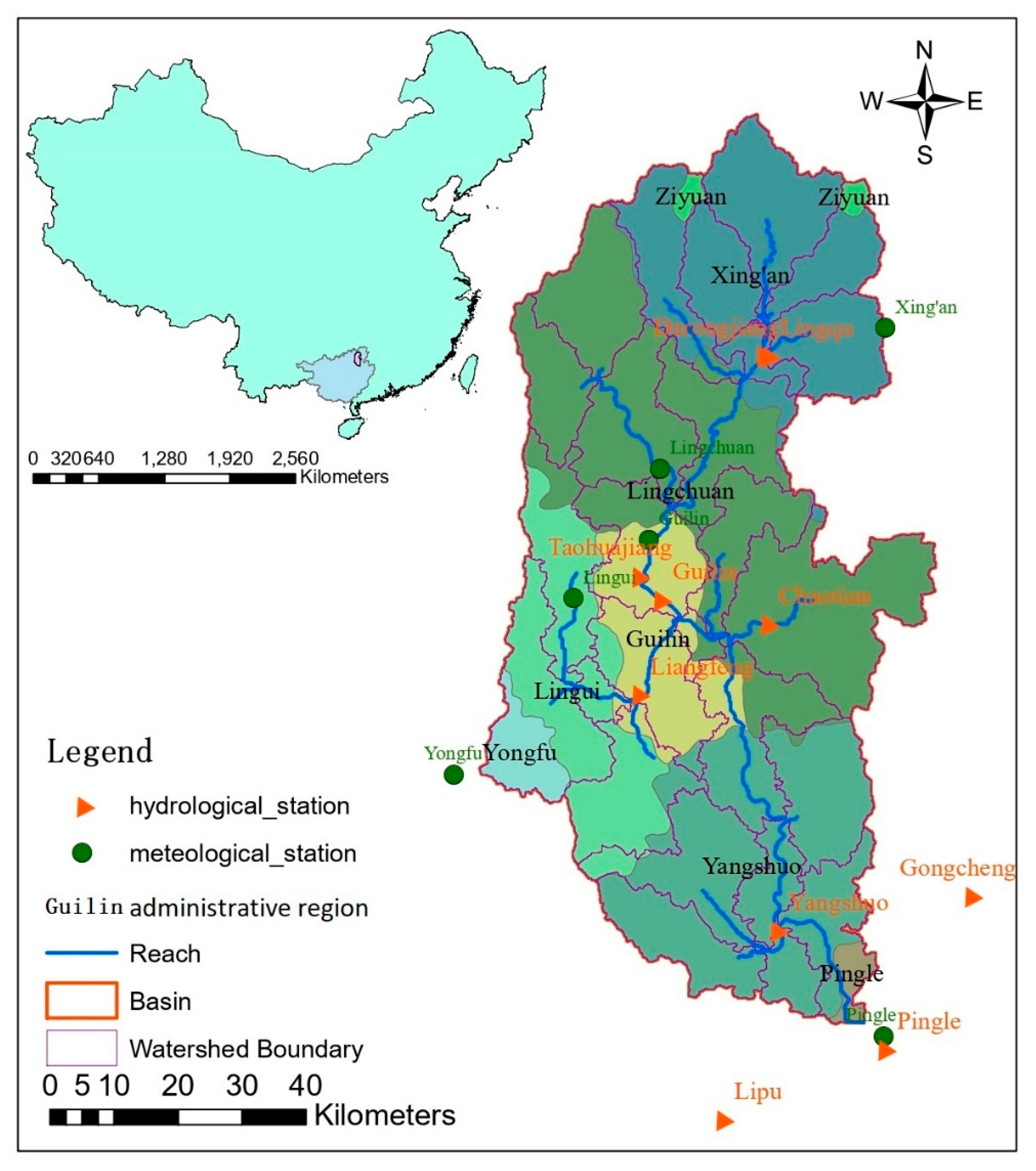
The Lijiang River Basin is located in Guilin city, Guangxi, which is the branch basin of the Pearl River Basin. It is enclosed between the latitude of 24°40′ N–26°00′ N and the longitude of 110°00′ E–110°40′ E. It is a karstic area with elevation ranging from 17 to 2111 m, with an average elevation of 1061 m. The average temperature of this area is 18 °C and the annual average rainfall is about 1500–2000 mm, and has a total area of 6375 km² (Figure 1). The detailed observed data of each weather or hydrological station are shown in Figure 1, and the meteorological and hydrological data are from http://data.cma.cn/ and the local hydrological yearbook over years. Although the Lijiang River Basin is located in South China, where the total amount of runoff from rainfall is relatively abundant, hydrological extremes, including droughts and floods, are frequent. The uneven distribution of the precipitation and runoff at both time and spatial scales is one of the effects of climate change in this basin [5]. Climatic events, such as droughts and floods, are closely affecting people lives and local economic development. Therefore, assessing the hydrological response to complicated climate changes is of great necessity.

The input data for SWAT modeling included the digital elevation model (DEM), hydrological, and meteorological data. The DEM data of the shuttle radar topography mission (SRTM) with resolution of 1 × 1 m were obtained from http://www.gscloud.cn. Hydrological data, including observed streamflow, land use, and soil data, were retrieved from the local hydrological yearbook and resource and environment data cloud platform (http://www.resdc.cn). Soil data were from the harmonized world soil database (HWSD) and their parameters were determined by the soil–plant–atmosphere–water (SPAW) tool. Climate data included both observed and GCM data, containing precipitation, maximum/minimum temperature, relative humidity, sunshine duration, and wind speed. Precipitation data were used to simulate the runoff, while others were used to simulate the potential evapotranspiration. The climate data of both observed and GCM were all at a daily scale. The observed data were from the meteorological stations presented in Figure 1, and GCMs were based on the fifth assessment report (AR5) of Intergovernmental Panel on Climate Change (IPCC) and developed several GCM data (http://www.ipcc-data.org/sim/gcm_monthly/AR5/index.html) of both historical and RCPs. Considering there are dozens of GCM outputs within IPCC and it is unrealistic to assess all of the GCM outputs, we used three GCMs (BNU-ESM, IPSL-CM5A-MR, and MIROC5) in this study, and three future RCPs (RCP2.6, RCP4.5, RCP8.5) were used. These three GCMs included all three RCPs and were presented just as an example to analyze the bias correction process and give a reference on how to correct the bias of other GCMs. The GCM outputs were corrected with observed data for the historical period of 1964–2005. Then, the corrected method was applied to the future period of 2016–2055.

2.2. Bias correction and Evaluation of GCM Outputs

2.2.1. Overview of Bias Correction Methods

Before setting up SWAT, the GCM outputs were preprocessed. GCMs often show significant biases including systematic model errors if compared with observed variables, especially precipitation and temperature [30]. To fully assess the future impacts of climate change on hydrological process, GCM is an effective tool to generate future climate patterns. In contrast to climate reanalysis, GCMs used for climate change impact assessment do not have the aim to fully represent observed daily values of meteorological variables. Instead, they try to represent climatological patterns, such as mean, trend, and seasonality. The reason is that GCM for reanalysis tries to meet initial conditions closely, but GCM for climate change assessment tries to follow boundary conditions. The SWAT model is forced by the original GCM simulations against the observed data. Bias correction is not required if there are small biases between simulated and observed data; otherwise, it is required as it is not suitable for hydrological modeling [18]. However, GCMs are usually based on climatological assumptions that usually emerge some non-ignorable errors compared with observed data. The original purpose of bias correction is, therefore, to make the GCM output close to the corresponding observed data as much as possible to decrease the errors of GCM outputs.

Table 1. Equations of multiple bias correction methods and corresponding symbol definition.

Correction Methods	Mathematical Equations		Coverage	References
Linear Scaling (LS)	$P_{cor}^{LS}\left(t\right)=P_{GCM}\left(t\right)\times \frac{{\mu }_m\left(P_{obs}(t)\right)}{{\mu }_m\left(P_{GCM}(t)\right)}$ $T_{cor}^{LS}\left(t\right)=T_{GCM}\left(t\right)+\left[{\mu }_m\left(T_{obs}(t)\right)-{\mu }_m\left(T_{GCM}(t)\right)\right]$		Precipitation and Temperature	[17]
Local Intensity Scaling (LOCI)	$s=\frac{\mu \left(P_{OBS}|P_{OBS}\ge OBS,thres\right)-P_{OBS,thres}}{\mu \left(P_{GCM}|P_{GCM}\ge GCM,thres\right)-P_{GCM,thres}}$ $P_{cor}^{LOCI}(t)=\max \left(0,P_{OBS,thres}+s\left(P_{GCM}\left(t\right)-P_{GCM,thres}\right)\right)$		Precipitation	[17,31]
Empirical Cumulative Distribution Function (ECDF)	$F\left(x\right)={\displaystyle {\int }_0^{x}f(t|\alpha ,\beta )dt}=\frac{1}{{\beta }^{\alpha }\Gamma \left(\alpha \right)}{\displaystyle {\int }_0^x{t}^{\alpha -1}{e}^{-\frac{t}{\beta }}dt}x\ge 0;\alpha ,\beta >0$ $G(x)={\displaystyle {\int }_{-\infty }^{x}g\left(t|\mu ,{\sigma }^2\right)}dt={\displaystyle {\int }_{-\infty }^x\frac{1}{\sqrt{2\pi }\sigma }}{e}^{-\frac{{(t-\mu )}^2}{2{\sigma }^2}}dt$ $P_{cor}^{ECDF}\left(t\right)=ecd{f}_{obs}^{-1}\left[ecd{f}_{GCM}\left(P\left(t\right)\right)\right]$ $T_{cor}^{ECDF}\left(t\right)=ecd{f}_{obs}^{-1}\left[ecd{f}_{GCM}\left(T\left(t\right)\right)\right]$		Precipitation and temperature	[15,32]
Variance Scaling (VARI)	$T_{cor}^{VARI}\left(t\right)=\left[T_{LS}\left(t\right)-{\mu }_m\left(T_{LS}\left(t\right)\right)\right]\cdot \frac{{\sigma }_m\left(T_{obs}(t)\right)}{{\sigma }_m\left[T_{LS}\left(t\right)-{\mu }_m\left(T_{LS}\left(t\right)\right)\right]}+{\mu }_m\left(T_{LS}\left(t\right)\right)$		Temperature	[33,34]
Symbols
P		Precipitation
μ()		Mean value
T		Temperature
s		Scaling factor
μ(A|B)		The mean value of A that satisfies the condition of B
F(x), f(t|α,β)		Cumulative distribution function and probability density function of Gamma distribution with two parameters α and β. Precipitation variable obey this distribution
G(x), g(t|μ,σ2)		Cumulative distribution function and probability density function of normal distribution with two parameters μ andσ2. Temperature variable obey this distribution
ecdf		Empirical cumulative distribution function
σ()		Standard deviation
Subscripts
cor		Corrected variables
obs		Observed variables
GCM		Original GCM variables
m		Monthly interval
thres		Threshold

lists the equations of multiple bias correction methods and corresponding references used in this study. A detailed description of each bias correction can be found in Supplementary Materials.

2.2.2. Hybrid Method

We also combined the bias correction methods to increase the correction precision, based on the assumption that the hybrid method may correct GCM output bias more efficiently compared with using only one method. We selected a combination of two of those methods in order to reduce computational cost. For each hybrid, the output of the initial correction becomes the input of the hybrid method. We use the hybrid of VARI&ECDF and LS&LOCI to correct temperature and precipitation, respectively, in this study, while LS&ECDF is used to correct both temperature and precipitation data. Thus, the developed hybrid bias correction is shown as follows:

$$T_{cor}^{VARI\&ECDF}\left(t\right)=ecd{f}_{OBS}^{-1}\left[ecdf\left(T_{cor}^{VARI}\left(t\right)\right)\right]$$

(1)

$$P_{cor}^{LS\&LOCI}\left(t\right)=\max \left(0,P_{obs,THRES}+s\left(P_{cor}^{LS}\left(t\right)-P_{LS,thres}\right)\right)$$

(2)

$$T_{cor}^{LS\&ECDF}\left(t\right)=ecd{f}_{OBS}^{-1}\left[ecdf\left(T_{cor}^{LS}\left(t\right)\right)\right]$$

(3)

$$P_{cor}^{LS\&ECDF}\left(t\right)=ecd{f}_{OBS}^{-1}\left[ecdf\left(P_{cor}^{LS}\left(t\right)\right)\right]$$

(4)

2.3. Description and Development of the SWAT Model

2.3.1. A brief Description of SWAT Model

The SWAT model is a typical semi-distributed model that has higher accuracy, which separates a large watershed into several sub-watersheds that consist of hydrological response units (HRUs) to increase its resolution. This includes a comprehensive coverage of basin behaviors and strong compatibility with a geographic information system (GIS) and diverse algorithms for hydrological processes [35]. For this study, we are evaluating the effects of climate change in runoff and evapotranspiration. SWAT calculates runoff based on the Soil Conservation Service [36] for estimating the amount of runoff under varying land use and soil types [37,38]:

$$Q_{surf}=\frac{{(R_{day}-0.2S)}^2}{R_{day}+0.8S}$$

(5)

$$S=25.4\left(\frac{1000}{CN}-10\right)$$

(6)

where Q_surf, R_day, S, and CN denote surface runoff (mm), rainfall depth (mm), retention parameter, and curve number. The curve number is determined by different types of land uses and soils that are classified by hydrological groups. For details on runoff calculations, see [38].

The groundwater runoff is presented as follows:

$$Q_{gw}=\frac{8000KH}{L^2}$$

(7)

where K, H, and L are the permeability coefficient (mm/d), depth of the diving surface (m), and the distance from the watershed of the sub-basin to the main channel (m), respectively.

Potential evapotranspiration (PET) was evaluated before calculating actual evapotranspiration using the Penman–Monteith equation:

$$E{T}_0=\frac{0.408\Delta \left(H_{net}-G\right)+\gamma \frac{900}{T+273}{u}_2\left(e_z^0-e_z\right)}{\Delta +\gamma \left(1+0.34u_2\right)}$$

(8)

where ET₀ is the potential evapotranspiration (mm/d), Δ is the slope vapor pressure curve (kPa/°C), H_net is the net radiation (MJ/m²/d), G is the soil heat flux density (MJ/m²/d), T is air temperature at 2 m height (°C), u₂ is wind speed at 2 m height (m/s), e_z⁰ and e_z are the saturation and actual vapor pressure of air at height z (kPa), and γ is the psychrometric constant (kPa/°C). Then, the actual evapotranspiration is calculated by evaporating the rainfall intercepted by the plant canopy and calculating the maximum amount of transpiration and sublimation/soil evaporation [38]. Therefore, evapotranspiration is determined by many environmental variables including temperature, solar radiation, humidity, etc.

2.3.2. SWAT Model Setup

The Soil and Water Assessment Tool (SWAT) was developed to simulate the runoff of the watershed in both historical and future periods under different scenarios of climate change. In this study, we used ArcSWAT2012, which is the extensional toolbar of ArcGIS 10.2 to setup the SWAT model. The simulated runoff of the historical period was used to calibrate and validate the performance of the SWAT model, while projected GCM outputs were used to predict the runoff in the future period. SWAT was developed based on the theory of the water balance equation [27,39]:

$$S{W}_t=S{W}_i+{\displaystyle \sum _{i=1}^t\left(P_i-Q_{i,surf}-E{T}_i-f_i-Q_{i,gw}\right)}$$

(9)

where SW_t and SW₀ (mm) are the soil water content at the tth and ith time interval, respectively. In this case, subscript i is the initial time. P_i (mm), Q_i,surf (mm), ET_i (mm), f_i (mm), and Q_i,gw (mm) are the precipitation, surface runoff, evapotranspiration, infiltration, and base flow at ith time interval. The SWAT model first divides the watershed into several small sub-basins according to the Digital Elevation Model (DEM) data and river system of the watershed. Then, the smallest unit of the watershed, HRU, is generated based on soil, land use, and slope. Each HRU contains these three elements. For this study, the watershed was divided in 29 sub-basins and 822 HRUs. Apart from DEM, land use, and soil data, SWAT also needs daily climate data including precipitation, maximum and minimum temperature, solar radiation, relative humidity, and wind speed to generate the hydrological process of a watershed. Additionally, SWAT also contains a weather generator model (WXGEN) that can generate water data or fill the gaps of observed climate data.

2.3.3. Model Performance Assessment

In this study, we used SWAT calibration and uncertainty program (SWAT-CUP) to evaluate the uncertainty and its performance of parameters by using the sequential uncertainty fitting (SUFI2) algorithm. We selected three years (1964–1966) for model warming up, while 1967–1975 and 1976–1984 were selected as calibration and validation periods, respectively. To evaluate the performance of the SWAT model, R², mean square error (MSE), and Nash–Sutcliffe Efficiency (NSE) were used. The value of R² and NSE range from −1 to 1 and from negative infinity to 1, respectively. In general, the closer the values of R² and NSE are to 1, the better the simulation effect is. If R² is greater than 0.6, while NSE is greater than 0.5, the simulation effect is satisfactory. If NSE is greater than 0.75, the simulation effect is efficient. The expressions of R² and NSE are shown below:

$$R^2=\frac{{\left[{\displaystyle \sum _{i=1}^n\left(Q_{obs,i}-\overline{Q_{obs}}\right)\left(Q_{sim,i}-\overline{Q_{sim}}\right)}\right]}^2}{{\displaystyle \sum _{i=1}^n{\left(Q_{obs,i}-\overline{Q_{obs}}\right)}^2}{\displaystyle \sum _{i=1}^n{\left(Q_{sim,i}-\overline{Q_{sim}}\right)}^2}}$$

(10)

$$MSE=\frac{{\displaystyle \sum _{i=1}^n{\left(Q_{obs,i}-Q_{sim,i}\right)}^2}}{\mathrm{var}\left(Q_{obs,i}\right)}$$

(11)

$$NSE=1-\frac{{\displaystyle \sum _{i=1}^n{\left(Q_{obs,i}-Q_{sim,i}\right)}^2}}{{\displaystyle \sum _{i=1}^n{\left(Q_{obs,i}-\overline{Q_{obs}}\right)}^2}}$$

(12)

where $Q_{obs,i}$ and $Q_{sim,i}$ are the observed and simulated streamflow at ith time interval, respectively. $\overline{Q_{obs}}$ and $\overline{Q_{sim}}$ are the average observed and simulated streamflow, respectively, during the entire evaluating period.

3. Results

3.1. Assessment of the GCM Outputs Using Multiple Bias Correction Methods

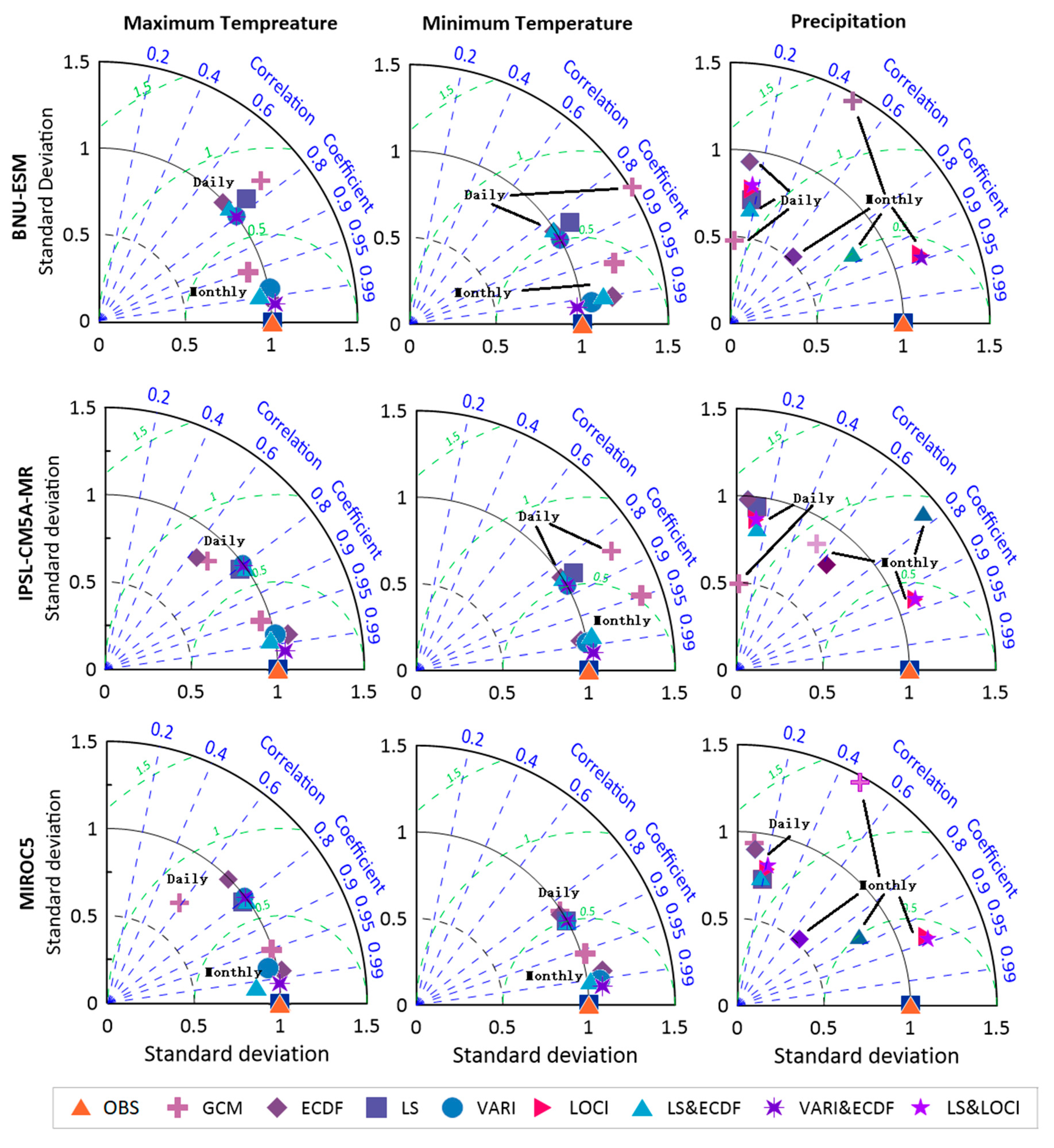
Due to the various number of GCMs that are unrealistic to analyze the bias correction methods for a full scale as there are dozens of GCM outputs, we selected and compared three GCM outputs for this study as the examples to test which bias method is relatively better. Figure 2 shows the Taylor diagram for the GCM corrections for daily data of 1964~2005. Measurements of evaluation include standard deviation (STD), root mean square error (RMSE), and correlation coefficient (CC). The CC of each original GCM of maximum temperature ranged from 0.6 to 0.8, while the CC of minimum temperature ranged from 0.8 to 0.9. The standard RMSE of both maximum and minimum temperature ranged from 0.5 to 1. Even if there was a relatively good simulation of original GCM of temperature, there was still an improvement of all the correction methods compared with original GCMs. To quantify the effect of the improvement, we also compared each improved percentage, which is shown in Figure 2. It can be seen from Figure 2 that for all three GCMs of temperature, each correction method is closer to the corresponding original GCMs and the effect of the hybrid method is better than either of the single methods in both CC and RMSE indexes.

Precipitation is more uncertain than temperature in terms of how dynamic the variable is, missed data, and record errors. Many factors determine the amount of precipitation, which is the main source of uncertainty. Moreover, when the frequency of precipitation data is higher, the error also increases. That is why the daily simulation result of the original GCM is poor compared with temperature, which is reflected by the CC of the original GCM only in the range from 0.01 to 0.1, and RMSE is larger than 1 (Figure 2). In addition, for the same climate variables, the monthly simulation is better than daily simulation results. Although the CC of the original GCM is very low, there is enough room for improvement. All the correction methods perform well in terms of CC. The CC is around 0.2 compared with the value before correction (0.01 to 0.1), which is the reason why the percentages of increase in CC have exceeded 100% (

Table 2. The percentage of change of correlation coefficient CC and root mean square error in each corrected method relative to the original daily precipitation as well as temperature of GCMs (unit: %).

Predictions	Correcting Methods	CC			RMSE
		BNU-ESM	IPSL-CM5A-MR	MIROC5	BNU-ESM	IPSL-CM5A-MR	MIROC5
Precipitation	LS	115.34	174.44	154.82	−6.70	−17.23	12.94
	ECDF	17.93	53.92	62.64	1.36	2.21	19.10
	LOCI	120.99	224.29	163.86	−9.47	−12.51	10.80
	LS&ECDF	154.53	351.29	87.03	−3.66	−8.17	21.19
	LS&LOCI	119.55	223.67	155.84	−10.66	−12.59	19.67
Maximum temperature	LS	10.31	22.55	38.93	12.32	14.09	16.69
	ECDF	2.90	4.65	5.20	11.36	6.39	4.08
	VARI	24.10	18.65	34.04	23.59	10.42	12.92
	LS&ECDF	12.09	24.20	40.46	16.61	14.65	17.01
	VARI&ECDF	24.88	20.03	35.54	24.13	15.51	18.91
Minimum temperature	LS	1.41	1.19	8.61	24.04	16.81	11.58
	ECDF	1.19	1.20	2.79	26.00	18.72	3.96
	VARI	8.50	8.56	8.81	35.94	26.77	11.77
	LS&ECDF	2.26	2.30	9.43	27.53	19.81	12.77
	VARI&ECDF	8.96	8.92	8.99	36.02	26.86	11.91

Notes: CC is the increase percentage and RMSE is the decrease percentage. For example, in BNU-ESM, the CC value of the maximum temperature of the LS method has increased by 10.31%, while RMSE value has decreased by 12.32%.

). However, the acute changes happen in RMSE in the BNU-ESM and IPSL-CM5A-MR models, which is reflected by the minus value which means the increasing trend of RMSE. Fortunately, the RMSE of MIROC5 performs well and all ECDF-corrected methods in each model are effective. For this phenomenon, we can contribute it for the uncertainty of the GCM itself that is determined by many factors, and the determinants may be also numerous and extremely complicated. From

Table 3. Nash–Sutcliffe efficiency (NSE) coefficient for both original and corrected daily GCM in the historical period of daily precipitation as well as temperature.

Correcting Methods	Precipitation			Maximum Temperature			Minimum Temperature
	BNU-ESM	IPSL-CM5A-MR	MIROC5	BNU-ESM	IPSL-CM5A-MR	MIROC5	BNU-ESM	IPSL-CM5A-MR	MIROC5
GCM	−0.64	−0.69	−0.67	0.31	0.50	0.45	0.38	0.53	0.68
LS	−0.30	−0.63	−0.27	0.47	0.63	0.62	0.72	0.75	0.81
ECDF	−0.15	−0.14	−0.10	0.45	0.43	0.41	0.69	0.69	0.70
LOCI	−0.36	−0.25	−0.33	/	/	/	/	/	/
VARI	/	/	/	0.59	0.60	0.59	0.80	0.80	0.81
LS&ECDF	−0.12	−0.09	−0.32	0.52	0.65	0.63	0.67	0.69	0.76
LS&LOCI	−0.27	−0.15	−0.37	/	/	/	/	/	/
VARI&ECDF	/	/	/	0.60	0.61	0.59	0.75	0.75	0.75

, we can see that the ECDF-corrected method performs also better in terms of NSE, and when it is combined with LS, the effect is greatly improved compared with LOCI and its hybrid with LS. It can also be seen from Table 3 that the value of all other correcting methods has greatly improved compared with the original GCM, which demonstrated that all the correcting methods have a positive effect. The effect of the hybrid method of precipitation can also be superimposed, except in the MIROC5 model and LS&LOCI method in the IPSL-CM5A-MR model. Although the value of NSE is slightly less than 0, the NSE value of the hybrid method is greatly better than the original and corresponding single GCM. This means the simulation of the process may have errors due to the uncertainty and complicated determinants, but the overall simulation result is reliable.

3.2. Calibration and Validation of the SWAT Model

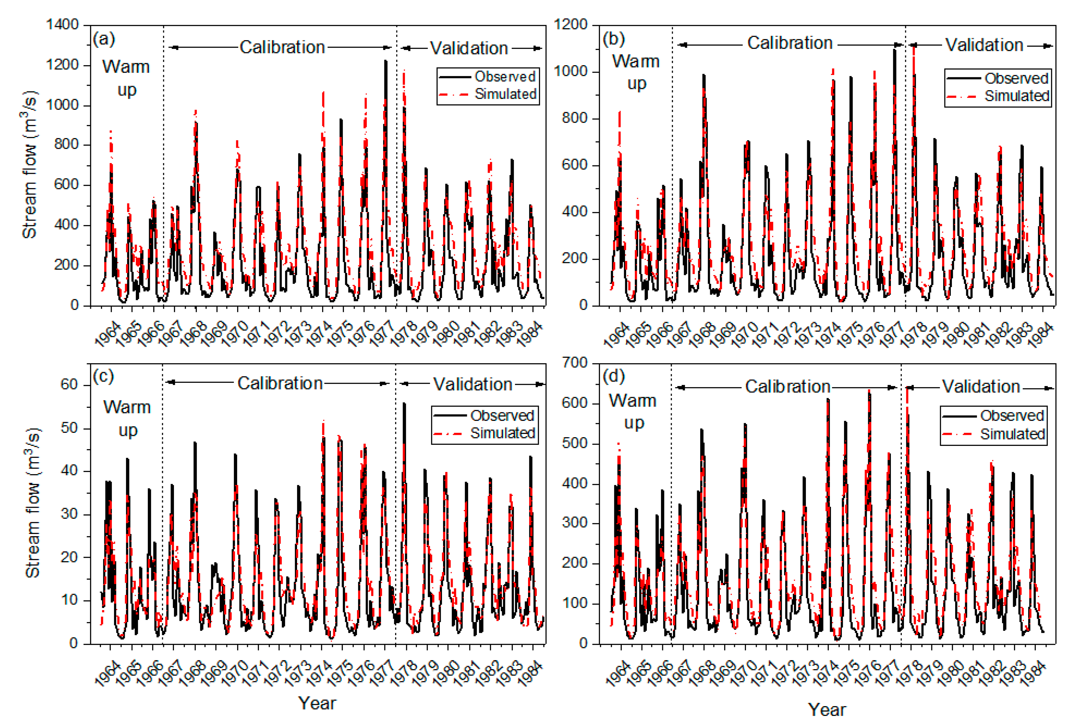
Calibration and validation processes were performed using monthly streamflow data given by the Pingle, Yangshuo, Lingqu, and Guilin hydrological stations. The first three years (1964–1966) were used to warm up and were not adopted in the model evaluation. The periods 1967~1975 and 1976~1984 were selected as calibration and validation periods. Visual comparison of the continuous data of observed and simulated streamflow in both calibration and validation periods is shown in Figure 3 and the statistical evaluation result is demonstrated in

Table 4. Simulation effect evaluation of monthly streamflow of four hydrological stations.

Hydrological Station	Calibration Period			Validation Period
	R2	MSE	NSE	R2	MSE	NSE
Pingle	0.87	0.23	0.77	0.82	0.25	0.71
Yangshuo	0.89	0.16	0.85	0.86	0.16	0.81
Lingqu	0.87	0.15	0.76	0.85	0.26	0.77
Guilin	0.87	0.16	0.82	0.86	0.20	0.82

. It can be seen that the R² values of four stations in both the two periods all exceeded 0.8 and NSE values also exceeded 0.7. Meanwhile, the MSE value in both periods was less than 0.3. It can also be indicated from Figure 3 that the monthly flow trends in the two periods for each hydrological station almost stayed the same, suggesting the simulation results have a relatively good performance.

3.3. Projected Climate Change Response to Hydrological Systems

3.3.1. Changes in Projected Precipitation and Temperature

Of all the single models, the performances of temperature seem to be similar, while those of precipitation vary from different similar models. For example, the ECDF method for monthly temperature performs poorer than other single methods (see Figure 2). This can be contributed to the statistical errors and the definition ambiguity of the drizzle rainfall, and less static errors of the observed temperature. However, the performance of the hybrid method of both monthly and daily scales of both precipitation and temperature is better compared with the single method in most cases. According to the correction results shown by Table 3, we found that precipitation correction performed the best in the LS&ECDF method in the IPSL-CM5A-MR method; the same GCM performed relatively better in temperature compared with the other two models. The LS&ECDF and VARI perform the best in maximum and minimum temperature, respectively. In this study, we used the abovementioned model and method to drive the SWAT model to simulate the hydrological variables.

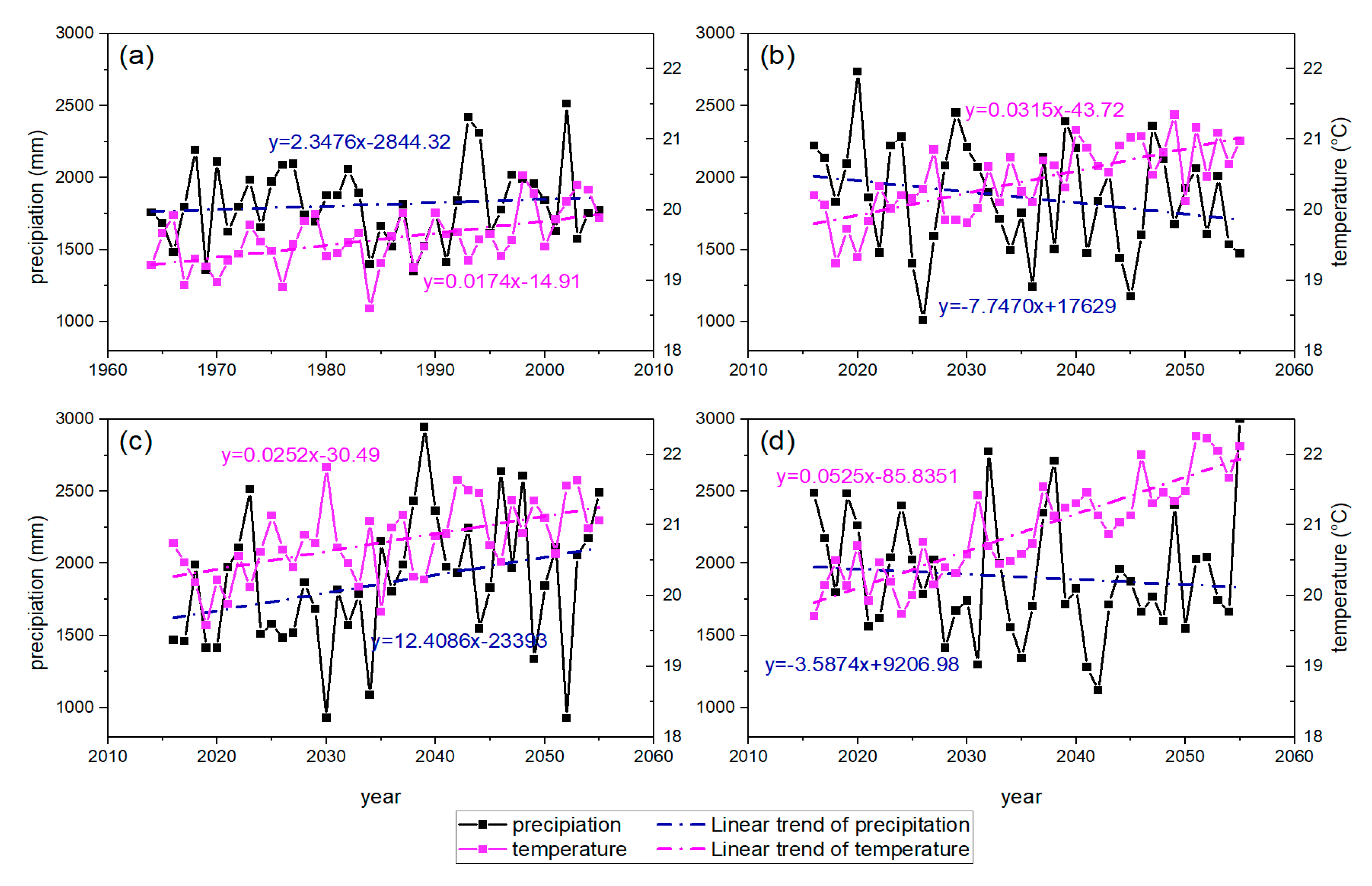
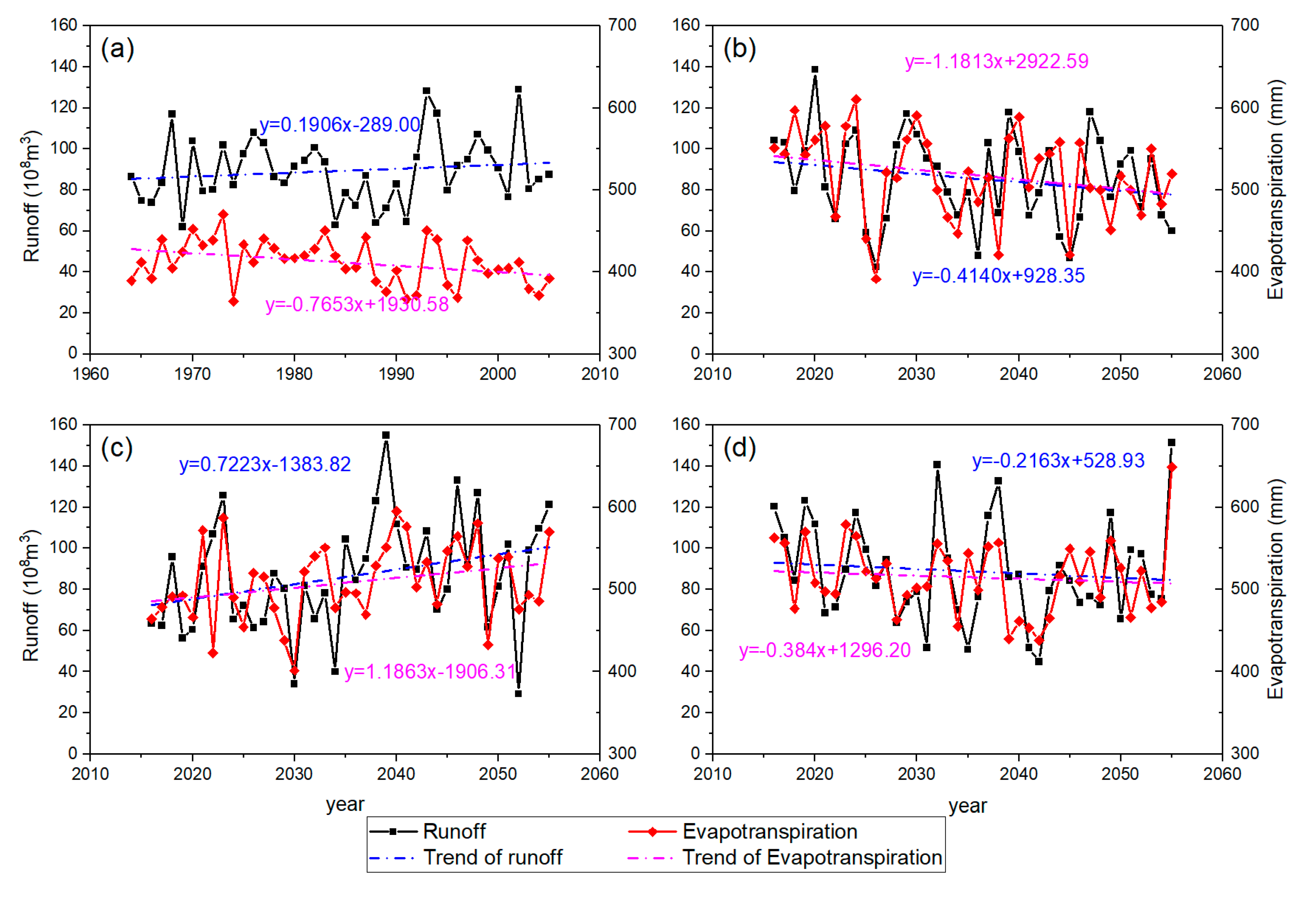
The multiyear trends of all the historical and future scenarios and the changes in the total amount of precipitation and temperature are shown in Figure 4 and

Table 5. The amount of annual precipitation and temperature during the historical and future period.

Hydrological Variables	Scenarios
	Historical	RCP2.6	RCP4.5	RCP8.5
Precipitation(mm)	1814.41	1860.18	1864.76	1904.89
Temperature(°C)	19.56	20.41	20.76	20.92

. In general, it presented increasing trends in all the scenarios in temperature and the increasing ratios of future scenarios (with the increase rate of 0.3, 0.25, and 0.53 °C per decade) are all greater than the historical periods (with the increase rate of 0.17 °C per decade). A greater ratio of temperature increase occurred in the RCP8.5 scenario compared with other RCP and historical scenarios. Similarly, the annual average temperature demonstrated the same change as the multiyear trend. Moreover, no matter from a multiyear trend or annual average perspective, the effect of RCP8.5 is the most obvious. Unlike the multiyear trend of temperature, the multiyear precipitation change reflects the increasing trend only in historical and RCP4.5 scenarios, with the increasing rate of 23.48 and 124.09mm per decade. However, the descending trend in RCP8.5 (77.47mm per decade) is less than that in RCP4.5 (35.87mm per decade). Although there is a descending trend in both RCP2.6 and RCP8.5 scenarios, the annual average precipitation in both scenarios is greater than that in the historical period. Besides, the increasing percentage change in RCP8.5 is greater than any of the other scenarios, which presents the same phenomenon as temperature in these two points.

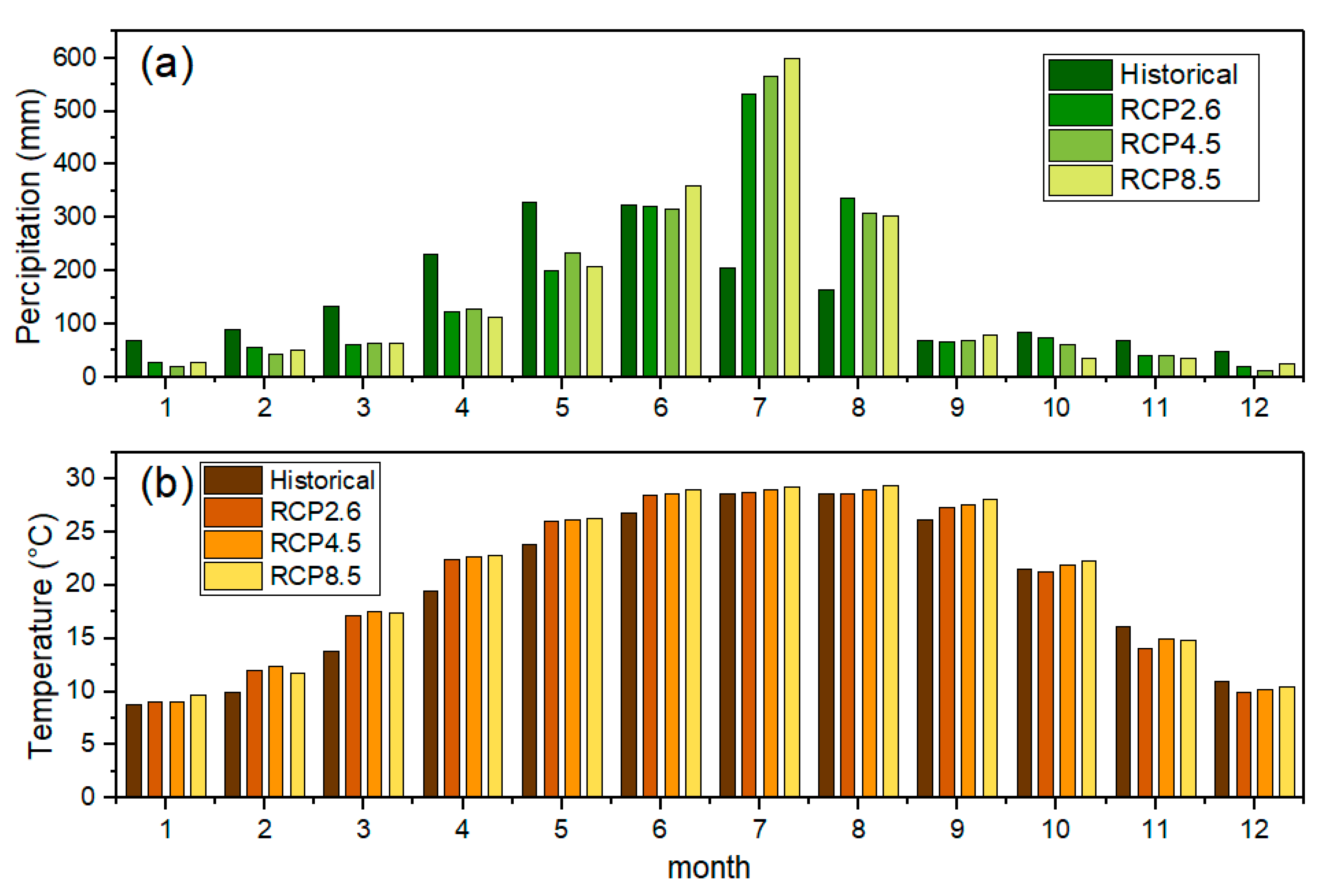
Figure 5 presents the monthly distribution of precipitation and temperature for each scenario, and it can be seen that the annual monthly temperature in future scenarios is always greater than the historical period except in November and December. The increasing rate presents a relatively obvious ratio from March to June compared with other months. When comparing with different future scenarios, the monthly temperature in RCP4.5 and RCP8.5 is always greater than RCP2.6. When it comes to precipitation, it is quite different from temperature. The precipitation in future scenarios increased in flood seasons, especially in July and August, and the rest of the months presented a decreasing trend. The temporal distribution of precipitation seems to be more uneven and the peak precipitation is increased and delayed. This means the peak precipitation happens in May with its value of about 350 mm in the historical period, while that in future scenarios has changed to about 550 mm and happened in July. This distribution change is likely to be manifestations of climate change.

3.3.2. Changes in Future Runoff and Evapotranspiration

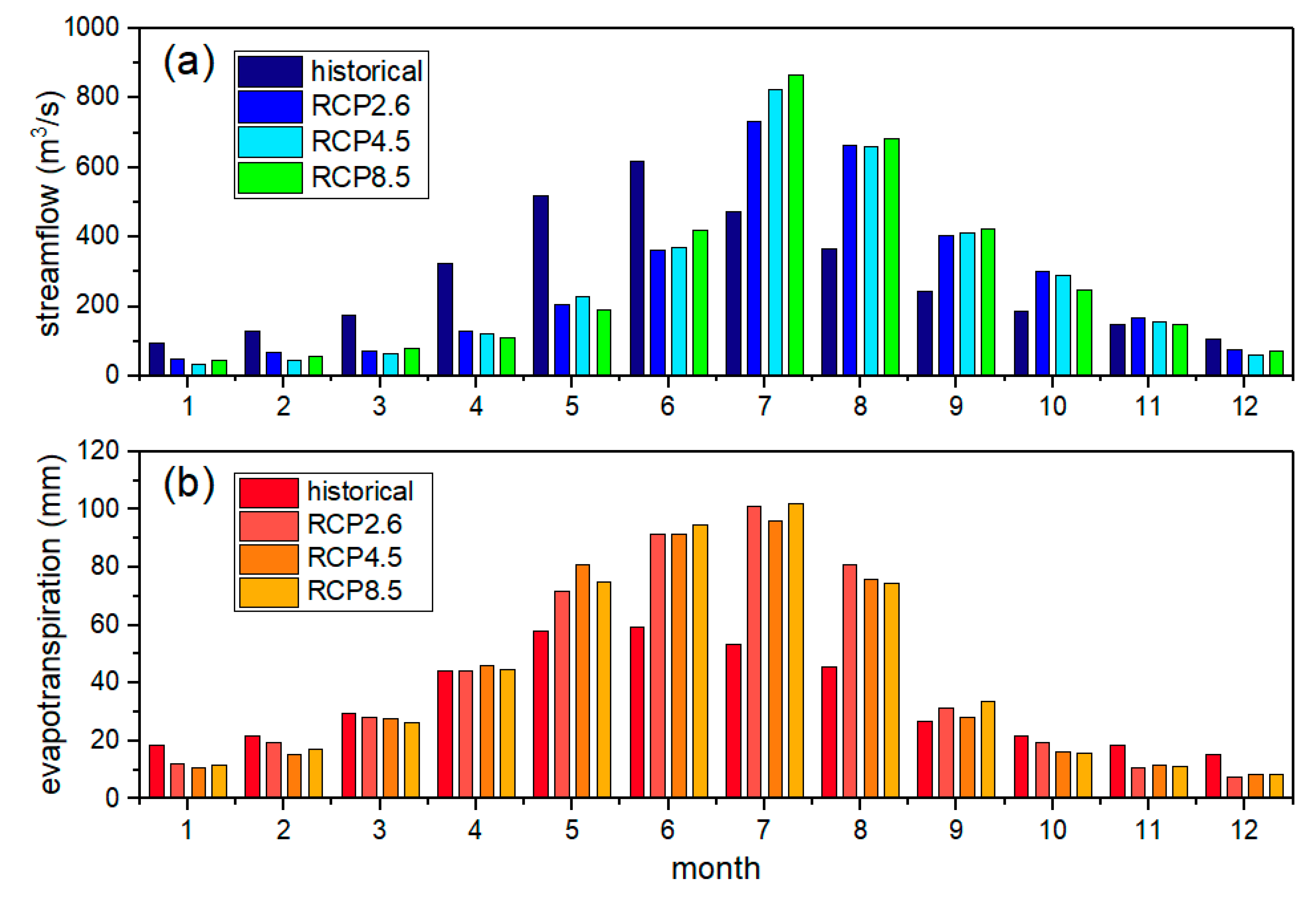
Figure 6 shows the multiyear trend of runoff and evapotranspiration of both historical and future periods based on three scenarios. These results showed the comprehensive effects of climate change based on the different emission scenarios. It can be seen from Figure 6 that the multiyear trend of runoff presents the descending trend in RCP2.6 and RCP8.5, while it showed an increasing trend in RCP4.5 and the historical period. The descending rate in RCP2.6 is slightly greater (4.1 × 10⁸ m³ per decade) than in RCP8.5 (2.2 × 10⁸ m³ per decade), while the increasing rate in RCP4.5 is greater (7.2 × 10⁸ m³ per decade) than in the historical period (1.9 × 10⁸ m³ per decade). This happens because the precipitation in the corresponding RCP scenarios is the same trend. However, RCP itself in the future scenarios is not the real-time trend that is based on several assumptions; therefore, different RCPs as well as GCMs and trends of either increase or decrease are both possibilities. The total amount of runoff in future cases is also more than that in the historical case (

Table 6. The amount of annual runoff and evapotranspiration during the historical and future period.

Hydrological Variables	Scenarios
	Historical	RCP2.6	RCP4.5	RCP8.5
Runoff (108 m3)	85.26	90.61	92.48	94.64
Evapotranspiration (mm)	411.83	508.45	514.57	518.15

). That means the total runoff in the future has also increased and the maximum amount of runoff occurs under RCP8.5. The changes are similar with that of precipitation (see Table 5, the annual average precipitation in future scenarios is more than that in historical scenarios). When focusing on the monthly distribution of runoff (Figure 7a), it showed a similar change as precipitation. The runoff will experience relatively positive changes in mid-period and later-period flood seasons (June to November) and negative changes in other periods, and the effect under RCP8.5 is more visible compared with other future scenarios in the mid-period flood season. Besides, the peak value is much greater and appears later compared with the historical period, suggesting the annual distribution of runoff is changed and becoming more uneven under the impacts of climate change.

The multiyear trends of evapotranspiration are the same as runoff in future scenarios, and this is even reflected in the increasing or decreasing rates. That is, the trend of evapotranspiration under RCP2.6 and RCP8.5 is decreasing while that in RCP4.5 is increasing, which is the same as the corresponding scenarios of runoff. Additionally, the decreasing rate in RCP8.5 (3.8 mm per decade) is also slightly less than in RCP2.6 (11.8 mm per decade). The annual average evapotranspiration in the future period is much greater than in the historical period (Table 6). This happens because the temperature in future scenarios is increasing greatly due to climate change, and the evapotranspiration will increase as temperature increases according to the Penman–Monteith equation. When comparing different future scenarios, the highest and the lowest increase ratio occurs in RCP8.5 and RCP2.6, respectively. The monthly distribution of evapotranspiration is also changed under the impact of climate change. We can see from Figure 7b that the evapotranspiration in flood seasons in all future scenarios is more than that in the historical period. The effect is obvious, especially in flood seasons from May and August. For non-flood seasons, it is either less than or keeps pace with historical periods. It is observed that the distribution of evapotranspiration is also changed and becomes uneven under climate change in each scenario.

4. Discussion

4.1. Comparison of Different Bias Correction Methods

Research on the impact of climate change has become popular in the last few decades. However, it is of great necessity to correct the GCM bias in that there will be systematic error in subsequent runoff simulating without bias correction. According to the previous studies in this field, the effect of GCM itself and the ECDF method of bias correction perform relatively well in higher latitudes and elevations where there is less precipitation, which brings about less uncertainty compared with humid and subtropical areas [1,16]. For low latitude and monsoon areas where there may be more precipitation with more uncertainties, the NSE value would be a little smaller but near zero so the model is still reliable. Additionally, the time interval also affects the NSE value, as monthly or average daily precipitation performs more perfectly than long-term daily data [16]. From this point of view, the results can also support the validity of the bias correction method used in this study.

According to the correction results (Table 3), the ECDF-corrected method performs better than the LOCI-corrected and LS-corrected method. This result is also validated in other research works, where the study area has similar climate conditions [15,32]. The change of precipitation is nonlinear and the LS method will not correct as perfectly as we expected. LOCI is independent of distribution compared with ECDF in that its scaling factors are calibrated on mean values of precipitation, and features instabilities in estimating the process of temporal variability. Therefore, it cannot correct the error adequately when the data are significantly curved and intensity-dependent [33]. ECDF is corrected based on the distribution of the long-term observed data, which is respectively representative and closer to the observed distribution data. That is also the reason why when LOCI is combined with LS, the simulation is poor compared with the hybrid method of LS&ECDF. Temperature simulating is much better than precipitation because of its lower uncertainty and determinants, and variance is smaller than precipitation. This is reflected by the greater value of NSE in temperature than precipitation, which means the model is reliable from both the overall and process perspective. Moreover, there is no sudden change in temperature as it is relatively stable, whereas the rainfall occurs with a certain probability that is difficult to quantify. That is why the value of RMSE in precipitation has an acute change. However, there is a normal change in MIROC5 so GCM itself also has uncertainty. Therefore, choosing a proper correcting method and GCM is also a key point before hydrological modeling. Additionally, the VARI-corrected method performs better than the LS-corrected method because VARI is the extension of LS as it considered both mean and variance of the total sample, which can be comprehended as the combination of linear and variable scaling [34,35]. Meanwhile, other hybrid methods perform also greater than corresponding single methods in both precipitation and temperature other than some exceptions, which means the effect of hybrid methods performs better than single methods to some extent, although it may not work in all the scenarios absolutely. After all, the sample size of climate data is too large and uncertainty is more likely to emerge, and it also has regional specificities. Therefore, the results are still valuable and provides a good reference to similar studies.

4.2. Variations of Hydrological Variables Caused by the Impacts of Climate Change

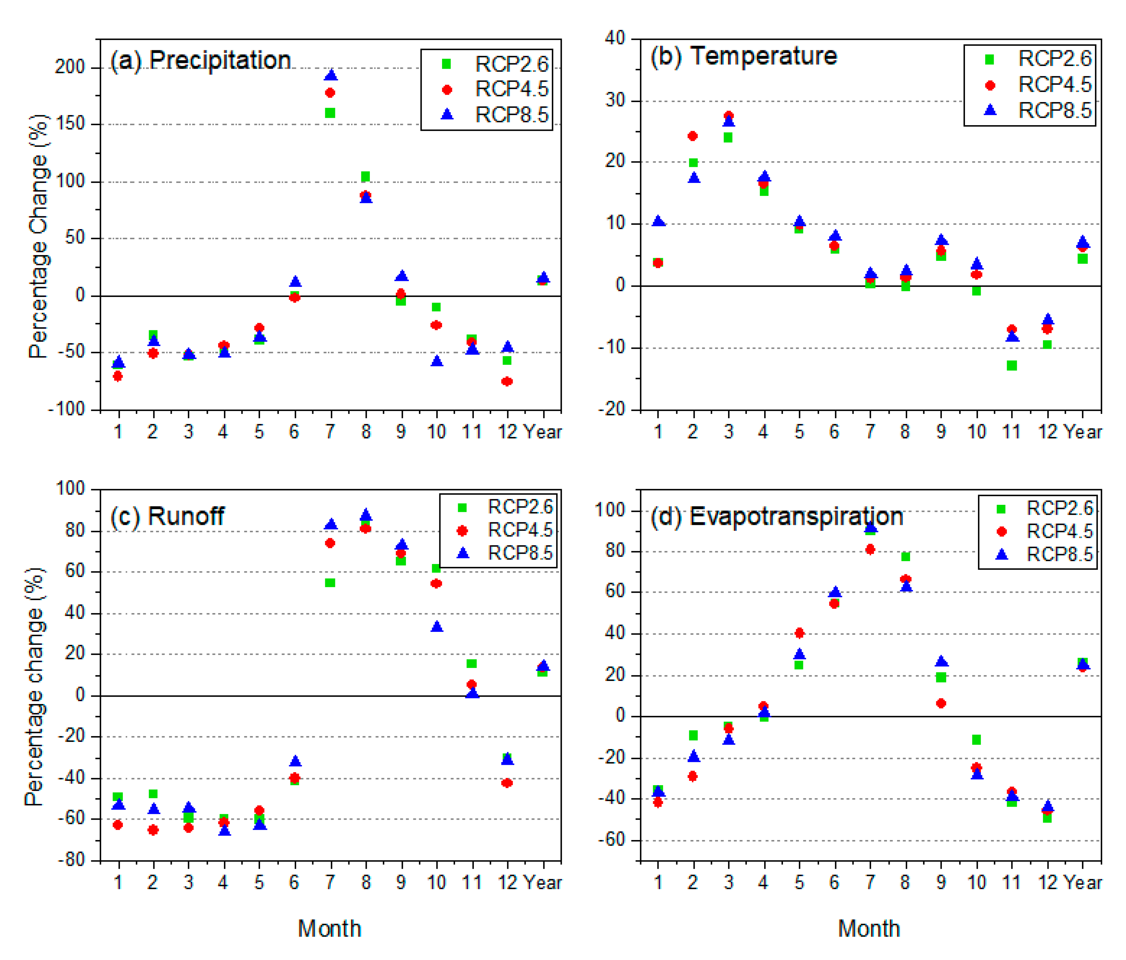
In general, the impacts of climate change showed intense temporal heterogeneity of hydrological variables in this study. According to the theoretical basis provided by [38], the amount of runoff is determined by the precipitation and condition of the underlying surface and evapotranspiration is determined mainly by temperature, humidity, and solar radiation. The annual average changes of evapotranspiration in 2016–2055 have increased by about 20% in three future scenarios, which can be mainly contributed to the changes of temperature, because the annual temperature has also increased about 1 °C (Figure 8b,d). There is no doubt that global warming is in process and will last for decades [2,27], and it is also the same with Lijiang River Basin. Both the multiyear trend of temperature (Figure 4) and the absolute temperature are increasing, contributing to the relatively large increasing ratio of evapotranspiration. The increasing temperature also contributes to the increasing value of evapotranspiration (about 100 mm, see Figure 5). Previous studies also indicated that continuous global warming will experience the growth of evapotranspiration compared with the past (Luo et al., 2019; Bibi et al., 2016). However, the changes in monthly temperature and evapotranspiration do not completely match (Figure 8b,d); for example, the increasing change in evapotranspiration in July and August is greater than that of temperature in the same period. This is probably because evapotranspiration is not only determined by temperature, but also solar radiation and humidity, as the solar radiation in these two months is much larger than other months, which brings about uncertainty factors to some extent. The evapotranspiration also varies in different climate scenarios. For example, its value in RCP8.5 (518.15 mm) is higher than those in RCP2.6 (508.45 mm) and 4.5 (514.51 mm) (see Table 6). This is easy to understand because a higher concentration of CO₂ emission occurs in the RCP8.5 scenario, which is likely to accelerate the greenhouse effect, which accelerates the increase in temperature, which contributes to the increasing evapotranspiration. There is no doubt that in the study area located in South China, sunshine duration is longer than other areas, especially in summer, as it is close to the equator. Yet, one thing is certain: the total amount of evapotranspiration is increasing compared with the historical period under the impact of climate change.

Climate change is also reflected in the changes more in temperature, but also in precipitation. Our results showed that annual average precipitation has increased (Table 5 and Figure 8a), which is consistent with other studies with similar conditions of the study area [27]. Simultaneously, the distribution of the monthly precipitation has also changed, reflected by the sharp increase in rainfall in the flood season (May to September) and decrease in the non-flood season (October to next April) (Figure 8a) as well as the delay of the peak occurrence time (Figure 5a), which may consequently lead to greater floods in the future flood season and frequent drought events in the non-flood season. Consequently, similar changes will also occur in the distribution of runoff (Figure 8c). Therefore, the stakeholders of water resources management should take measures towards this issue like floodwater utilization—gathering the water resources in flood seasons to meet the needs in dry seasons. With the increasing precipitation, runoff is also increasing compared with baseline. Although evapotranspiration increases in future scenarios, the study area is a monsoon and humid area where annual precipitation is larger than evapotranspiration and future precipitation is also increasing as we speculated. Moreover, the dual effect of increasing precipitation and temperature can accelerate streamflow. This is validated by its value under different climate scenarios. The runoff in RCP8.5 is 94.64 × 10⁸ m³, which is less than that under RCP2.6 (90.61 × 10⁸ m³) and RCP4.5 (92.48 × 10⁸ m³), in which the precipitation and temperature are also lower compared with RCP8.5. Thus, we can speculate that the increasing trend of the annual amount of runoff will happen during 2060–2100. Zhang et al. [27] also showed that the change in streamflow is influenced by the simultaneous changes of precipitation and temperature and showed similar results in the 2020s, 2050s, and 2080s; their study area is also a monsoon area that is similar to the area in this study. In contrast, other studies [1,35,40,41] with alpine and dry areas, where evapotranspiration is more than precipitation, show a decreasing trend in runoff.

4.3. Changing Hydrological Variables Compared with Other Areas

We compared the hydrological response of climate change in the Lijiang River Basin with other related watersheds. As presented in this study, the annual average of temperature, evapotranspiration, and precipitation will increase in the future. The results are also validated in Piao et al. [42], which performed a similar study in Southern China. Although runoff has slightly decreased in the study area, it is affected by both increasing precipitation and evapotranspiration, and the theorical runoff could either increase or decrease. Related research obtained similar findings. For example, Zhang et al. [27] assessed the hydrological response of climate change in the Xin River Basin, which is also a monsoon and humid area and is also located in Southern China. This study showed the increasing change of precipitation and temperature, and the result of runoff is close to baseline, which showed similar changes in this study. The monthly precipitation and runoff distribution are also similar to this study as the peak flow occurs in summer, although the peak value of the Xin River Basin is in early- and mid-summer, while in this study, it occurs in mid-summer. The annual average runoff in the 2080s is more than that in the 2050s, and runoff in the 2050s is also greater than in the 2020s. Stagge et al. [43] has also demonstrated the increasing trend of annual runoff in the Potomac River located in Mid-Atlantic US, with an average increasing percentage of only 2.7%, 4.0%, and 4.3% in short-, mid-, long-term future periods.

When comparing with the areas that are different from our study area, the results are different. In this case, different conditions are usually with higher altitude and drier climates, and their annual precipitation is usually less than most monsoon areas [44]. However, most arid areas have more runoff compared with humid and monsoon areas, in that there is more snow accumulation in winter and snow melt in spring as temperature rises [1,12]. Therefore, hydrological elements have heterogeneity in multiple areas of different conditions. In general, in humid and monsoon areas, especially in southern China, the precipitation and runoff usually demonstrate the seasonal characteristics and annual precipitation is usually greater than arid areas with higher altitude, such as the typical areas of Western China and Central Asia.

5. Conclusions

In this study, we analyzed several GCM outputs by using both single and combined bias correction methods and selected the most suitable corrected GCM as input for the SWAT model. The historical (1964–2005) and future scenarios (2016–2055) with three RCPs were used to simulate the precipitation, temperature, evapotranspiration, and runoff. The hydrological variables indicated great heterogeneity, especially in monthly distribution. The following conclusions can be drawn in this study:

(1) All the correction methods have a positive effect compared with the original GCM. For precipitation, the ECDF-corrected method performs better than LOCI and LS, and the effect of the hybrid method containing ECDF is also more obvious than that containing LOCI. The correcting method except ECDF is less obvious in the BNU-ESM and IPSL-CM5A-MR model in terms of RMSE, but it is better in the MIROC5 model, which demonstrates the GCM itself has uncertainty and complicated determinants. For temperature, the simulating result is better than precipitation as it has less uncertainty, and VARI performs the best among the single methods.

(2) The hybrid method of correcting precipitation and temperature has the superimposed effect in terms of NSE in most cases of the study area, which means the effect of the hybrid method is more obvious than either of the single methods to some extent. Therefore, choosing a proper GCM and correcting method is also a key procedure, and this paper can provide a reference for the method of bias correction.

(3) Both the trend of temperature changes in multiyear and its annual average value are increasing and the maximum rate occurs in the RCP8.5 scenario. The monthly distribution of temperature also increased in each month. The trend of precipitation changes in multiyear showed an increasing trend in RCP4.5, while other future scenarios showed a decreasing trend, but the annual average precipitation is increasing relative to baseline, and the maximum changing rate is under RCP8.5. The monthly distribution trend of precipitation is uneven, reflected by the increase in mid-flood season, decrease in other seasons, increase in peak flow, and delay of the peak occurrence time.

(4) The annual evapotranspiration increased in all three future scenarios, but the multiyear trend increase only occurred in RCP4.5. Its positive changes also occurred in flood seasons and kept pace with historical periods in non-flood seasons. The multiyear trend of runoff increased only in RCP4.5 and the annual average of runoff decreased slightly compared with baseline, but in future scenarios, the multiyear average runoff has increased compared with baseline and the maximum runoff occurs under RCP8.5. The monthly distribution of runoff is similar to precipitation and also showed the uneven trend in the future. As the precipitation continues increasing compared with baseline and raising the temperature can accelerate the streamflow, the annual average runoff in the further future may increase.

Although this research determined the hydrological response to climate change for the Lijiang River Basin, there are some issues that require further discussion; for example, the uncertainty of GCM outputs analysis and the performance of several GCM outputs that best fit the study area. The standard should be various and comprehensive and not limited to R² or NSE. Another valuable endeavor would be using more samples of GCM outputs. The best bias correction methods may differ from multiple GCM outputs as GCM outputs are generated based on several assumptions that cause uncertainties, and the uncertainties analysis based on more samples can be conducted in our further studies.

References

- Luo, M.; Liu, T.; Meng, F.; Duan, Y.; Bao, A.; Xing, W.; Feng, X.; de Maeyer, P.; Frankl, A. Identifying climate change impacts on water resources in Xinjiang, China. Sci. Total Environ. 2019, 676, 613–626. [Google Scholar] [CrossRef]
- Intergovernmental Panel on Climate Change (IPCC). AR5 Synthesis Report: Climate Change; Cambridge University Press: Cambridge, UK, 2014. [Google Scholar]
- Li, F.; Zhang, Y.; Xu, Z.; Teng, J.; Liu, C.; Liu, W.; Mpelasoka, F. The impact of climate change on runoff in the southeastern Tibetan Plateau. J. Hydrol. 2013, 505, 188–201. [Google Scholar] [CrossRef]
- Ruelland, D.; Ardoin-Bardin, S.; Collet, L.; Roucou, P. Simulating future trends in hydrological regime of a large Sudano-Sahelian catchment under climate change. J. Hydrol. 2012, 424, 207–216. [Google Scholar] [CrossRef]
- Lin, Q.X.; Wu, Z.Y.; Singh, V.P.; Sadeghi, S.H.R.; He, H.; Lu, G. Correlation between hydrological drought, climatic factors, reservoir operation, and vegetation cover in the Xijiang Basin, South China. J. Hydrol. 2017, 549, 512–524. [Google Scholar] [CrossRef]
- Almazroui, M.; Islam, M.N.; Saeed, F.; Alkhalaf, A.K.; Dambul, R. Assessing the robustness and uncertainties of projected changes in temperature and precipitation in AR5 Global Climate Models over the Arabian Peninsula. Atmos. Res. 2017, 194, 202–213. [Google Scholar] [CrossRef]
- Meinshausen, M.; Smith, S.J.; Calvin, K.; Daniel, J.S.; Kainuma, M.; Lamarque, J.; Matsumoto, K.; Montzka, S.; Raper, S.; Riahi, K. The RCP greenhouse gas concentrations and their extensions from 1765 to 2300. Clim. Chang. 2011, 109, 213–241. [Google Scholar] [CrossRef] [Green Version]
- Xin, X.; Zhang, L.; Zhang, J.; Wu, T.; Fang, Y. Climate change projections over East Asia with BCC-CSM1.1 climate model under RCP scenarios. J. Meteorol. Soc. Jpn. 2013, 91, 413–429. [Google Scholar] [CrossRef] [Green Version]
- Chen, J.; Frauenfeld, O.W. Surface air temperature changes over the twentieth and twenty-first centuries in China simulated by 20 CMIP5 models. J. Clim. 2014, 27, 3920–3937. [Google Scholar] [CrossRef]
- Siew, J.H.; Tangang, F.T.; Juneng, L. Evaluation of CMIP5 coupled atmosphere-ocean general circulation models and projection of the Southeast Asian winter monsoon in the 21th century. Int. J. Climatol. 2014, 34, 2872–2884. [Google Scholar] [CrossRef]
- Fonseca, A.R.; Santos, J.A. Predicting hydrological flows under climate change: The Tamega Basin as an analog for the Mediterranean region. Sci. Total Environ. 2019, 668, 1013–1024. [Google Scholar] [CrossRef]
- Anjum, M.N.; Ding, Y.; Shangguan, D.; Ahmad, I.; Ijaz, M.W.; Farid, H.U.; Yagoub, Y.E.; Zaman, M.; Adnan, M. Performance evaluation of latest integrated multi-satellite retrievals for Global Precipitation Measurement (IMERG) over the northern highlands of Pakistan. Atmos. Res. 2018, 205, 134–146. [Google Scholar] [CrossRef]
- Chu, J.T.; Xia, J.; Xu, C.Y.; Singh, V.P. Statistical downscaling of daily mean temperature, pan evaporation and precipitation for climate change scenarios in Haihe River of China. Theor. Appl. Climatol. 2010, 99, 149–161. [Google Scholar] [CrossRef]
- Birkinshaw, S.J.; Guerreiro, S.B.; Nicholson, A.; Liang, Q.; Quinn, P.; Zhang, L.; He, B.; Yin, J.; Fowle, H.J. Climate change impacts on Yangtze River discharge at the Three Gorges Dam. Hydrol. Earth Syst. Sci. 2017, 21, 1911–1927. [Google Scholar] [CrossRef] [Green Version]
- Piani, C.; Haerter, J.O.; Coppola, E. Statistical bias correction for daily precipitation in regional climate models over Europe. Theor. Appl. Climatol. 2010, 99, 187–192. [Google Scholar] [CrossRef] [Green Version]
- Luo, M.; Liu, T.; Meng, F.; Duan, Y.; Frankl, A.; Bao, A.; De Maeyer, P. Comparing bias correction methods used in downscaling precipitation and temperature from regional climate models: A case study from the Kaidu river basin in Western China. Water 2018, 10, 1046. [Google Scholar] [CrossRef] [Green Version]
- Teutschbein, C.; Seibert, J. Bias correction of regional climate model simulations for hydrological climate-change impact studies: Review and evaluation of different methods. J. Hydrol. 2012, 456, 12–29. [Google Scholar] [CrossRef]
- Hashino, M.; Yao, H.; Yoshida, H. Studies and evaluations on interception processes during rainfall based on a tank model. J. Hydrol. 2002, 255, 1–11. [Google Scholar] [CrossRef]
- Steele-Dunne, S.; Lynch, P.; McGrath, R.; Semmler, T.; Wang, S.; Hanafin, J.; Nolan, P. The impacts of climate change on hydrology in Ireland. J. Hydrol. 2008, 356, 28–45. [Google Scholar] [CrossRef]
- Gao, C.; Liu, L.; Ma, D.; He, K.; Xu, Y.P. Assessing responses of hydrological processes to climate change over the southeastern Tibetan Plateau based on resampling of future climate scenarios. Sci. Total Environ. 2019, 664, 737–752. [Google Scholar] [CrossRef]
- Gao, J.; Holden, J.; Kirkby, M. Modelling impacts of agricultural practice on flood peaks in upland catchments: An application of the distributed TOPMODEL. Hydrol. Process. 2017, 31, 4206–4216. [Google Scholar] [CrossRef] [Green Version]
- Chiew, F.H.S.; Siriwardena, L. Estimation of SIMHYD Parameter Values for Application in Ungauged Catchments 1; University of Melbourne: Melbourne, Australia, 2005. [Google Scholar]
- Harlan, D.; Wangsadipura, M.; Munajat, C.M. Rainfall-runoff modeling of Citarum Hulu River basin by using GR4J. Proc. World Congr. Eng. 2010, 2, 1–5. [Google Scholar]
- Martina, M.L.V.; Todini, E.; Liu, Z. Preserving the dominant physical processes in a lumped hydrological model. J. Hydrol. 2011, 399, 121–131. [Google Scholar] [CrossRef]
- Wi, S.; Ray, P.; Demaria, E.M.C.; Steinschneider, S.; Brown, C. A user-friendly software package for VIC hydrologic model development. Environ. Model. Softw. 2017, 98, 35–53. [Google Scholar] [CrossRef]
- Wang, Z.G.; Liu, C.M.; Wu, X.F. A review of the studies on distributed hydrological model based on DEM. J. Nat. Resour. 2003, 18, 168–173. [Google Scholar]
- Zhang, Y.; You, Q.; Che, C.; Ge, J. Impacts of climate change on streamflows under RCP scenarios: A case study in Xin River Basin, China. Atmos. Res. 2016, 178–179, 521–534. [Google Scholar] [CrossRef]
- Chattopadhyay, S.; Edwards, D.R.; Yu, Y.; Hamidisepehr, A. An Assessment of Climate Change Impacts on Future Water Availability and Droughts in the Kentucky River Basin. Environ. Process. 2017, 4, 477–507. [Google Scholar] [CrossRef]
- Xu, Y.-P.; Zhang, X.; Ran, Q.; Tian, Y. Impact of climate change on hydrology of upper reaches of Qiantang River basin, East China. J. Hydrol. 2013, 483, 51–60. [Google Scholar] [CrossRef]
- Christensen, J.H.; Boberg, F.; Christensen, O.B.; Lucas-Picher, P. On the need for bias correction of regional climate change projections of temperature and precipitation. Geophys. Res. Lett. 2008, 35. [Google Scholar] [CrossRef]
- Schmidli, J.; Frei, C.; Vidale, P.L. Downscaling from GCM precipitation: A benchmark for dynamical and statistical downscaling methods. Int. J. Climatol. J. R. Meteorol. Soc. 2006, 26, 679–689. [Google Scholar] [CrossRef]
- Jakob Themeßl, M.; Gobiet, A.; Leuprecht, A. Empirical-statistical downscaling and error correction of daily precipitation from regional climate models. Int. J. Climatol. 2011, 31, 1530–1544. [Google Scholar] [CrossRef]
- Chen, J.; Brissette, F.P.; Poulin, A.; Leconte, R. Overall uncertainty study of the hydrological impacts of climate change for a Canadian watershed. Water Resour. Res. 2011, 47. [Google Scholar] [CrossRef]
- Chen, J.; Brissette, F.P.; Leconte, R. Uncertainty of downscaling method in quantifying the impact of climate change on hydrology. J. Hydrol. 2011, 401, 190–202. [Google Scholar] [CrossRef]
- Zhang, H.; Huang, G.H.; Wang, D.; Zhang, X. Multi-period calibration of a semi-distributed hydrological model based on hydroclimatic clustering. Adv. Water Resour. 2011, 34, 1292–1303. [Google Scholar] [CrossRef]
- Soil Conservation Service (SCS). National Engineering Handbook, Hydrology, Section 4; Soil Conservation Service; US Department of Agriculture: Washington, DC, USA, 1956. [Google Scholar]
- Rallison, R.E.; Miller, N. Past, present, and future SCS runoff procedure. In Rainfall-Runoff Relationship/Proceedings, Proceedings of the International Symposium on Rainfall-Runoff Modeling, Starkville, MS, USA, 18–21 May 1981; Singh, V.P., Ed.; Water Resources Publications: Littleton, CO, USA, 1982. [Google Scholar]
- Neitsch, S.L.; Arnold, J.G.; Kiniry, J.R.; Williams, J.R. Soil and Water Assessment Tool Theoretical Documentation Version 2009; Texas Water Resources Institute, Texas A&M University: College Station, TX, USA, 2011. [Google Scholar]
- Arnold, J.G.; Srinivasan, R.; Muttiah, R.S.; Williams, J.R. Large area hydrologic modeling and assessment part I: Model development. J. Am. Water Resour. Assoc. 1998, 34, 73–89. [Google Scholar] [CrossRef]
- Naz, B.S.; Kao, S.C.; Ashfaq, M.; Rastogi, D.; Mei, R.; Bowling, L.C. Regional hydrologic response to climate change in the conterminous United States using high-resolution hydroclimate simulations. Glob. Planet. Chang. 2016, 143, 100–117. [Google Scholar] [CrossRef] [Green Version]
- Fang, G.; Yang, J.; Chen, Y.; Zhang, S.; Deng, H.; Liu, H.; De Maeyer, P. Climate change impact on the hydrology of a typical watershed in the Tianshan Mountains. Adv. Meteorol. 2015, 2015. [Google Scholar] [CrossRef] [Green Version]
- Piao, S.; Ciais, P.; Huang, Y.; Shen, Z.; Peng, S.; Li, J.; Zhou, L.; Liu, H.; Ma, Y.; Ding, Y.; et al. The impacts of climate change on water resources and agriculture in China. Nature 2010, 467, 43–51. [Google Scholar] [CrossRef]
- Stagge, J.H.; Moglen, G.E. A nonparametric stochastic method for generating daily climate-adjusted streamflows. Water Resour. Res. 2013, 49, 6179–6193. [Google Scholar] [CrossRef]
- Gao, G.; Chen, D.; Xu, C.Y.; Simelton, E. Trend of estimated actual evapotranspiration over China during 1960–2002. J. Geophys. Res. 2007. [Google Scholar] [CrossRef] [Green Version]
Figure 1.
Location of Lijiang River Basin with digital elevation model DEM, and meteorological and hydrological stations.
Figure 2.
Taylor diagrams comparing the original and corrected GCMs of different methods of precipitation and minimum and maximum temperature of both daily (1960.1.1–2005.12.31) and monthly (1960.1–2005.12).
Figure 3.
SWAT model calibration and validation results: comparison between simulated and observed monthly stream flows of four hydrological stations: (a) Pingle; (b) Yangshuo; (c) Lingqu; (d) Guilin.
Figure 4.
Yearly changing trend of precipitation and temperature of both historical and future period: (a) historical, (b) RCP2.6, (c) RCP4.5, and (d) RCP8.5.
Figure 5.
Monthly changes of hydrological variables in the whole study area in both historical (1964–2005) and future (2016–2055) period: (a) precipitation; (b) temperature.
Figure 6.
Yearly changing trend of runoff and evapotranspiration of both historical and future period: (a) historical, (b) RCP2.6, (c) RCP4.5, and (d) RCP8.5.
Figure 7.
Monthly changes of hydrological variables in the whole study area in both historical (1964–2005) and future (2016–2055) period: (a) streamflow; (b) evapotranspiration.
Figure 8.
Percentage changes in all hydrological variables.