1. Introduction
Climate tends to change at a slow pace; however, this does not mean that climate is not prone to experiencing short-term fluctuations or anomalies at seasonal or longer timescales [
1,
2]. For instance, with rainfall being an essential meteorological variable subject to climate system components (e.g., to the atmosphere), it can fluctuate around the average without causing the long-term rainfall average itself to change [
3]. This phenomenon is a clear example of climate variability, which refers to variations in the mean state and in other statistics on spatio-temporal scales [
4]—such as extreme hydrological events withdrawing too far away from long-term values. These variations result from atmospheric and oceanic circulation, which in turn is caused mostly by differential heating of the sun on Earth. Globally, atmosphere–ocean circulations may cause extreme rainfall events or even exacerbate local and regional rainfalls from season to season or year to year time periods [
5,
6].
Furthermore, it is acknowledged that a higher global surface temperature (GTS) increases the intensity of extreme rainfall events more greatly than that of average rainfalls [
7,
8,
9,
10]. For the North Atlantic sector, a substantial portion of the GTS variability is associated with the North Atlantic Oscillation (NAO), a hemispheric meridional oscillation with one centre of action over the subtropical Atlantic and the other near Iceland. The NAO refers to large-scale changes in atmospheric pressure at sea level (SLP), and thus, changes in GTS and rainfall [
11]. The NAO-related impacts on climate, particularly in winter, extend from eastern North America to Greenland and from northwestern Africa over Europe [
12]. Despite this large-scale circulation pattern being non-linear in how it reacts, it has been shown that it has largely influenced the occurrence of extreme rainfalls during its negative and positive phases, leading to stronger climate responses depending on the location in the North Atlantic or the proximity to the Atlantic Ocean (e.g., [
13,
14,
15]). For instance, when the NAO is in its negative phase, pressure anomalies are not so noticeable, producing stronger-than-average easterlies. Throughout the same negative NAO phase, warmer and wetter conditions characterise the northwestern Atlantic and southern European regions, whereas colder and drier than average conditions are seen in Northern Europe [
16]. Contrasting patterns occur during the NAO positive phases with generalised opposite conditions.
A remarkable feature of the NAO is the upward seasonal and annual trend shown since the late 1980s, with high positive records [
17]. However, this period has also been characterised by persistent negative NAO index (NAOI) values that seem to be unprecedented in the daily observational record [
18]. Some of these persistent negative anomalies have occurred since the 2009/2010 winter. In this period, the NAO swung into an extreme negative phase, escaping the long-term upward trend, fostering unusually wet conditions and apparently promoting extreme rainfall events in some North Atlantic regions, most notably in the European Macaronesia—e.g., in the Canary Islands and the Madeira Archipelago [
19]. Thus, monitoring the state of the NAO at shorter timescales (e.g., at daily scale) can improve the understanding of the climate variability with regard to rainfall extremes—as performed in this research work for a small island of the Madeira Archipelago, namely, Madeira Island—and be crucial for better short-term water resource management and planning.
Although the effects of the NAO persist for some months, the closest relationships are shown in the winter period, accounting for more than one-third of the total rainfall variance from December through February [
20,
21]. The formulae for the relationships between NAO and extreme rainfalls in this research work are therefore based on rainfalls above a quantile threshold occurring in those months and on previous NAOI to such events, i.e., on the occurrence of unprecedented NAOI values and extreme rainfalls with a time lag.
In this study, statistical models are developed to assess (i) how persistent NAO conditions alone can model extreme daily rainfall and (ii) if considering a multivariate approach—specifically a bivariate one between NAO and rainfall—improves the assessment of climate variability in the small Portuguese island of Madeira. This island is the appropriate setting for this analysis as it shows an overall mild climate but different microclimates due to its geographical location, sharp topography, and effect of the mountain ridge and of the North Atlantic Ocean. In the mountain region of Madeira, particularly during the winter season, heavy rainfalls have triggered flash floods, landslides and debris flows (the so-called “
aluviões”) [
22] in periods that coincide with perturbation of Earth’s energy balance. In addition, during the winter of 2009/2010, the most negative NAO records were registered for the last 160 years clearly outside of the long-term averages or trends [
23] along with extreme rainfall, which in turn led to numerous hazards and causalities for the same winter period. Although rare, hydrological extreme events, such as extreme rainfall, have caused loss of life and had negative economic and social impacts on the island. Therefore, the need for appropriate statistical models of extreme hydro-meteorological events linked to large-scale atmospheric phenomena, i.e., teleconnection, becomes clear, particularly in the current context of a more recent pronounced climate variability.
Extreme rainfall events have often been linked to the strong climatic conditions and climate variability in the North Atlantic and adjacent land areas. For instance, Wilby et al. [
24] investigate correlations between extreme rainfall and other climatic variables in the British Isles in relation to decadal variations in the atmospheric circulations—in terms of the NAOI—during winter. Tramblay et al. [
25] provide a regional assessment of trends and variability in extreme rainfall over Maghreb countries—the western and northern African countries of Morocco, Tunisia, Algeria, and Libya—showing that extreme rainfalls exhibit a strong spatial variability and are moderately correlated with large-scale atmospheric patterns such as the NAO, but also with the El Niño Southern Oscillation (ENSO), as described in [
26]. Further, the NAO has also been found to affect the intensity and frequency of extreme rainfall. Queralt et al. [
27] analysed 102 rain gauges with daily records over Spain and the Balearic Islands from 1997 through 2006, arguing that NAO exerts a clear effect on the increasing intensity of total and extreme rainfall rates in northern and westernmost Spanish regions and on the increasing rainfall frequency in central and southwestern areas. Specifically for Madeira Island, very few studies have been undertaken to understand the influence of the NAO on extreme rainfall. As an example, Espinosa et al. [
18] focus on short-term climatic fluctuations in the NAO (e.g., daily NAOI) and claim the existence of systematic evidence of statistical dependence over Madeira between exceptionally daily negative NAOI (−NAOI) records and extreme regionalised rainfalls, based on a bivariate extremal dependence analysis, which is stronger in sustained NAOI year-long periods. It is in this context that the relevance of this study is emphasised by assessing some of the climate variability aspects.
Such an assessment was conducted with the use of copulas [
28] to model the bivariate dependence between daily NAOI and extreme daily rainfall in Madeira, from 1967/1968 to 2016/2017, assuming both variables exhibit different marginal behaviours. Copulas have been recently used to determine the conditional probabilities and return periods of multivariate problems. Wong et al. [
29] fitted a trivariate copula to drought characteristics, i.e., drought magnitude, duration and intensity, for some Australian rainfall districts. André and de Zea Bermudez [
30] analysed and characterised the dependence using copulas between daily maximum wind speeds observed in mainland Portugal and simulate daily maximum wind speeds produced by a numerical physical model. Gouveia-Reis et al. [
31] investigate the dependence of Madeira’s rainfall data and spatial variables (altitude, slope orientation, distance between rain gauges, and distance to the sea) within an extreme value copula approach through an analysis of maximum annual data. To the best of the authors’ knowledge, a more complex framework with at least one large-scale atmospheric pattern as a predictor—in this research work, the state of daily NAO—and extreme rainfall as a response variable has not yet been addressed.
The present paper is structured as follows. A brief description of the study area, the data used, and copula are given with a focus on bivariate return periods. The extreme winter daily rainfalls at six rain gauges in the island are first selected based on an empirical percentile as a threshold. A low-pass filter is applied to the daily NAOI series. The correlation between extreme rainfalls and previous smoothed NAOI, i.e., with a lag in between, is assessed. The bivariate observations for marginals selection and copula modelling are determined. Bivariate copula models for NAOI and extreme rainfalls are developed and compared. The selected copulas are then used to determine the bivariate joint and conditional return periods, in addition to univariate return periods, to assess the climate variability of the NAO and rainfall for Madeira Island from a multivariate perspective. The marginal and copula selection and the climate variability assessment are also discussed.
2. Physical Features of the Study Area
Madeira is the largest island of the Madeira Archipelago with an area of approximately 740 km
, a length of 58 km and a 23 km width. Centred at 32°75
N and 17°00
W, the small island of Madeira—according to its size [
32]—is completely shaped by volcanic materials, consisting of an enormous east-to-west (EW) oriented mass that is cut by deep valleys [
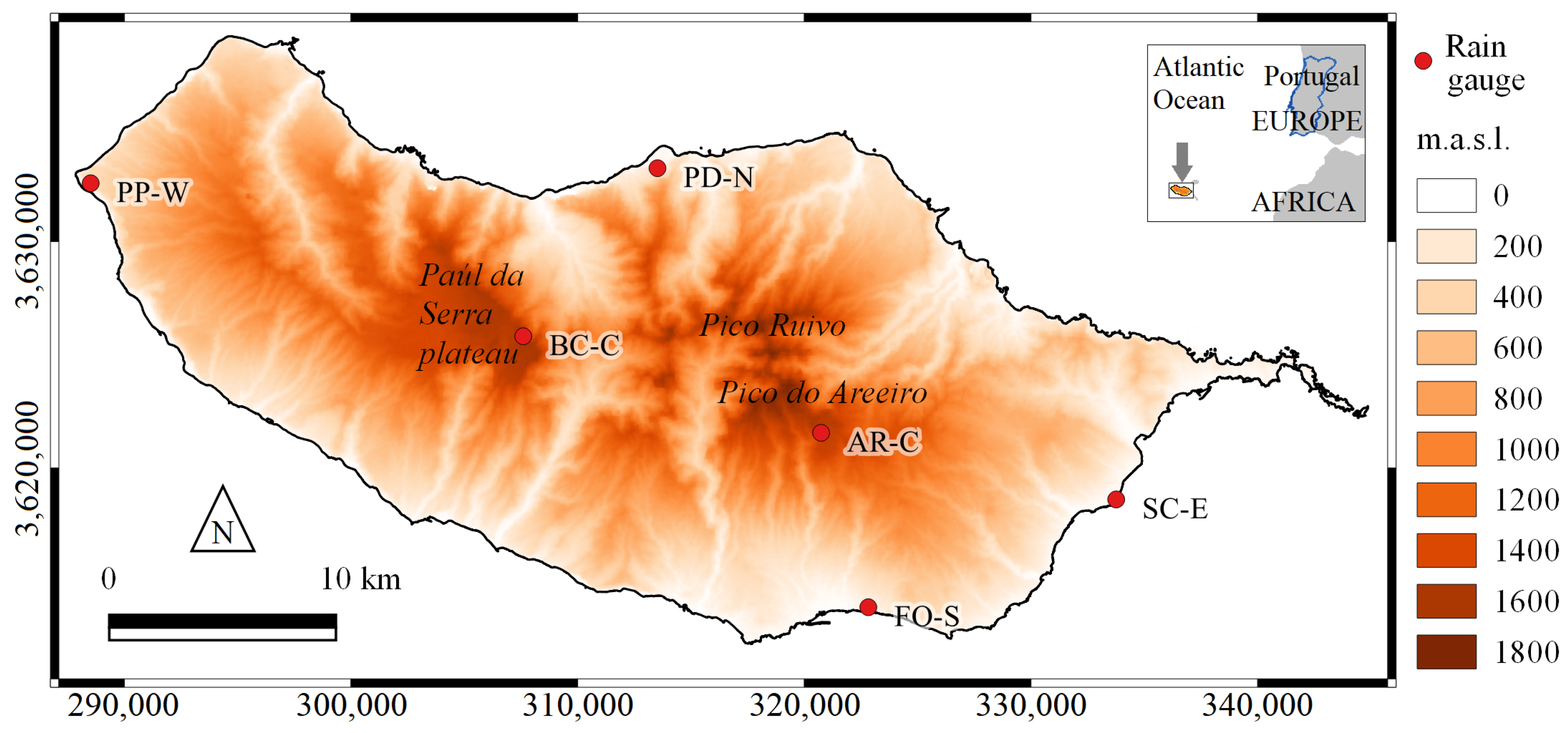
33]. Madeira has a mountain ridge that extends mainly along the central part of the island with the highest peaks in the eastern part, Pico Ruivo (1862 m.a.s.l.) and Pico do Areeiro (1818 m.a.s.l.), while the Paúl da Serra plateau (approx. 24 km
above 1400 m.a.s.l.) is located in the western part, as shown in
Figure 1. The abrupt orography of peaks and valleys, together with the North Atlantic effect, provide the island with a great variety of microclimates, mostly with a mild summer and winter, except for the highlands, where the lowest temperatures are registered [
34].
The rainfall regime over the Madeira is affected by local circulation and also by synoptic systems such as fronts and extratropical cyclones [
22]. The distribution of rainfall presents an evident seasonal pattern, thoroughly different between the rainy season, that extends from November to March, and the dry season, with insignificant rainfall amounts during July and August [
35]. The pronounced spatial variability of the rainfall in Madeira is determined mostly by the topography and the trade winds or easterlies—the permanent EW prevailing winds that flow in the Earth’s equatorial region [
36]—with higher amounts in the northeast (∼1600 mm year
) and central highlands (∼2300 mm year
) than in the western (∼800 mm year
) and southern regions (∼600 mm year
), as previously characterised by Espinosa and Portela [
37].
3. Materials and Methods
To assess the climate variability from 1 December 1967 to 28 February 2017, it was vital to derive some connected schemes of relationship or teleconnections to the NAO from extreme daily rainfall events. To this end, the rainfall daily data from December to February (DJF) of the following year were considered at six rain gauges of the island, with the expectation that different rainfall regimes would be identified due to their location: in the northern, southern, eastern and western slopes, and in the central ridge and plateau. The rainfalls above the 99th empirical percentile rank were considered as extreme rainfall events—following the recommendation of the Expert Team on Climate Change Detection, Monitoring and Indices (ETCCDMI) [
38]. Based on the considered period, the number of selected rainfalls is 90 consecutive days over 50 years. Out of the 4500 days of winter DJF rainfall at each rain gauge, the highest 45 rainfalls, i.e., 1%, were chosen as extreme rainfall events.
Different smoothed NAOI series were considered—by simple averages—relating to their running length,
m, and to the lag between the ending day of the smoothed series and the day of occurrence of each extreme rainfall event,
l. The Pearson linear correlation [
39] was applied to analyse the relationship between the smoothed and lagged values of NAOI and the selected extreme rainfalls events. Based on this correlation analysis, (i) the smoothing factor or low-pass filter [
40] of
m NAOI daily values and (ii) the number of lagged days,
l, between the end of the smoothed NAOI values and the occurrence of extreme rainfalls were selected. This analysis was based on the rainfall data at Areeiro rain gauge (AR-C in
Figure 1). This rain gauge is located at the central highlands, an area that highly contributes to the island’s fresh water availability and aquifer recharge due to the high rainfall and geological conditions prone to infiltration [
35]. The previous NAOI values (smoothed and lagged NAOI) based on the preceding correlation analysis were assigned to the extreme rainfalls. The
m and
l achieved based on AR-C were applied to the other five stations so that the final dataset for copulas modelling could be assembled.
Subsequently, the Wald–Wolfowitz runs test [
41] was used to test the null hypothesis
of independence for the observations of the final dataset (either NAOI values or extreme rainfalls). The second part of the methodology consisted of the bivariate analysis of NAOI as the “cause” of extreme rainfall using copulas by modelling such teleconnection. Finally, the concept of bivariate return period was applied for the events defined by the joint behaviour of pairs of the random variables adopted, i.e., daily NAOI and extreme daily rainfall. This was the core of the climate variability assessment for the island of Madeira.
3.1. Rain Gauge Data
The daily rainfall data at six representative rain gauges located at the central highlands (AR-C and BC-C), southern (FO-S), northern (PD-N), western (PP-W), and eastern (SC-E) slopes, were used—
Table 1 and
Figure 1. The data for the time-frame from December 1967 to February 2017 were made available by IPMA—Portuguese Institute for the Ocean and Atmosphere (
https://www.ipma.pt/en/, accessed on 20 January 2018). The data had some gaps that were filled, as described by Espinosa et al. [
42]. IPMA is the national authority in the fields of meteorology, aeronautical meteorology, climate, seismology, and geomagnetism, and an institution of reference at the international level also devoted to the promotion and coordination of scientific research. For each of the rain gauges, 4500 winter daily rainfall data were retrieved, i.e., 90 DJF daily values for 50 years (excluding leap year days).
3.2. North Atlantic Oscillation Index (NAOI) Data
The large-scale atmospheric characteristics were identified through the analysis of a synoptic meteorological index for the North Atlantic Oscillation, i.e., NAOI, at the daily scale, retrieved from the portal of the NOAA Physical Sciences Laboratory, NOAA PSL [
43]. The NAOI represents a pattern of low-frequency tropospheric height variability. This measure of pressure difference is based on centres of action of 500 millibars constant pressure (mb) height patterns. Note that these height fields are spectrally truncated to total wave number 10 in order to emphasise large-scale aspects of teleconnection. The calculation of this teleconnection index utilises the ESRL/PSD Global Ensemble Forecasting System Reforecast2 (GEFS/R) ensemble forecasts from the averaged region 55–70° N; 70–10° W, which in turn is subtracted from 35–45° N; 70–10° W. The NAOI daily records were utilised for the same period as in the case of daily rainfall (DJF, from 1967/1968 through 2016/2017), but also include the months of September, October, and November, prior to each December.
3.3. Bivariate Copula
The problem of specifying a probability model for dependent bivariate observations can be greatly simplified by expressing the corresponding joint distribution
in terms of its marginals,
and
, and an associated dependence function copula
C—introduced by Sklar [
44]—completely defined through the functional identity
.
C is a bivariate copula, hereafter copula. It is precisely the copula that captures the features of a joint distribution. Moreover, copulas measure the association and dependence structure properties connecting random variables. In this research work, a possible way of analysing bivariate data (NAOI,
X, and extreme rainfall,
Y) consisted of investigating the dependence function and the marginals separately. This approach was convenient for the climate variability assessment, as this allowed studying the dependence structure independently of any marginal effect. Regardless of the marginal laws involved, the analysis of this research work was focused on practical applications of modelling copulas for teleconnection and not on the equations involved. Nevertheless, the main mathematical descriptions related to the copula concept [
44] are presented next.
Definition 1. Let ; a copula is a bivariate function such that (1) uniform marginals: for u, , it holds that , and ; and (2) two-increasing: for , such that and , it holds that ; where is uniformly continuous on . Hereafter (respectively, ) will denote the marginal distribution functions of the random variables (respectively, ).
Theorem 1. (Sklar). Let be a joint distribution function with marginals and . Then, there exists a copula such thatfor all real x, y. If are continuous, then is unique; otherwise, is uniquely defined on Range () × Range (). Conversely, if is a copula and are distribution functions, then , given by Equation (1), is a joint distribution function with marginals and . The detailed proof of Sklar’s Theorem can be found in the work of Schweizer and Sklar [45]. In addition, since
is invariant under strictly increasing transformation of
X and
Y, by virtue of the Probability Integral Transform, the pair of random variables can be expressed as
, where
with
. With
U and
V being non-exceedance probabilities given by the marginal distribution functions, they are uniform on
, i.e.,
u and
u ref. [
46]. Hereafter,
is considered as the pair of NAOI and extreme rainfall variables—and also the pair
, respectively—having a direct practical meaning.
Given a bivariate distribution function
F with invertible margins
and
, a bivariate copula
for
is given by Equation (
3). Meta-elliptic copulas are symmetric and hence lower and upper tail dependence coefficients are the same.
The Archimedean copulas are more flexible than Meta-elliptic and can present lower or upper tail dependences, which are defined by Equation (
4):
where
is the generator function of the copula
C and
is a continuous and factually reducing function. The Meta-elliptic Gaussian and Student’s
t, and the Archimedean Clayton, Frank, and Gumbel, were tested to verify best fit.
Table 2 presents the formulations of the candidate copula families. When the Archimedean copula is rotated 180°, it is called a survival copula and can invert the predefined tail dependence to best fit the data.
3.3.1. Copula Parameter Estimation
The parameters for the candidate copula families were estimated considering the maximum likelihood MLE method, by choosing the Inference Functions from the Margins (IFM) method [
47]. The use of the IFM method requires previous fitting of marginal distribution functions to transform the variables’ values into the
interval.
3.3.2. Best-Fitted Copula
To compare the bivariate copula models from a number of families and choose the best-fitted model, the fit statistic AIC was used. First, all the candidate copulas, Gaussian, Student’s
t, Clayton, Frank, and Gumbel, were fitted using a maximum likelihood estimation, MLE. Then the AIC was computed for all copula families and the one with the minimum AIC was chosen. According to Brechmann and Schepsmeier [
48], for observations
and
with
, the AIC of a bivariate copula family
C with
parameter(s) is defined by Equation (
5):
where one parameter’s copulas has
and the two-parameter Student’s
t has
. The two-parameter copula was penalised in the minimisation of the AIC value to reduce possibility of overfitting due to the parsimony principle.
3.3.3. Bivariate Return Periods
In this subsection, the concept of a return period for events defined by their joint behaviour of pairs of random variables is introduced. This concept was applied to emphasise the particular facets of the dynamics of the considered NAOI—with particular emphasis on the negative phase of the NAO—and extreme rainfall phenomenon in Madeira Island. However, first, some necessary concepts are mathematically described as follows.
Among the several definitions of the return period, Shiau and Shen [
49] describe it as the average elapsed time between occurrences of the event with a certain magnitude or greater than a threshold. The higher the return period, the more exceptional the event is. The univariate return periods of NAOI and extreme rainfall, based on the concept of stochastic processes, are derived as follows. The return period, adapted from [
49,
50,
51], of the NAOI
or extreme rainfall
, is expressed as function of the expected interarrival time
E(
L) and of the cumulative distribution functions (CDFs) of the NAOI,
, and the extreme rainfalls,
, as defined in Equations (
6) and (
7), respectively (marginal distributions). Note that, in this case, T and
E(
L) are expressed in years. The
E(
L) was obtained by dividing the 45 bivariate events (based on the chosen extreme rainfalls) by the 50 analysed years, resulting in 0.9 year for each of the six rain gauges.
Assuming that the phenomenon studied here has a multivariate nature, the return periods of the bivariate distributed NAOI and extreme rainfall events were computed as joint and conditional return periods based on the works by Shiau [
52], but for drought analysis from a multivariate perspective in this case. Thus, the joint NAOI and extreme rainfall return period can be defined for
and
, as described in Equation (
8):
where
is the return period for
(NAOI) and
(extreme rainfall).
Analogously, the conditional return period was calculated for the case when NAOI is the cause of extreme rainfall, i.e., the return period of extreme rainfall given that the previous NAOI is lower than a certain threshold
. This conditional return period is calculated by Equation (
9):
Further discussion on the calculations and relationships between univariate, bivariate, and conditional return periods is out of the scope of this paper. However, this can be found in the work of Shiau [
52].
4. Results
The results are structured as follows. In
Section 4.1, the characteristics and temporal distribution of the 45 winter extreme daily rainfalls, from 1 December to 28 February of the following year (DJF), during the considered 50 years (1967/1968–2016/2017), are shown at each of the six adopted rain gauges in Madeira Island. Then, in
Section 4.2, the correlations between both the non-smoothed (
) and smoothed daily NAOI series (after applying a low-pass filter
) and extreme daily rainfall events at AR-C (Areeiro rain gauge) are presented under the assumption that the NAO is the major stressor of extreme rainfall. Different running lengths,
m, and time lags,
l, were tested for the NAOI, aiming at identifying the coupled series of previous NAOI and extreme rainfalls with maximum correlation. The
m and
l based on AR-C were then applied to the other five rain gauges, thus making up the final dataset with 45 bivariate observations at the six rain gauges in total. Subsequently, the overall strength of the association between previous NAOI and extreme rainfalls is described. In
Section 4.3, the estimation of the bivariate joint distributions along with the copulas’ construction are shown. Finally, in
Section 4.4, the results of the bivariate return periods based on the chosen copulas for the NAO and extreme rainfall phenomena are presented.
4.1. Extreme Daily Rainfall Distribution Analysis
The analysis of the winter (DJF) extreme daily rainfalls from 1967/1968 through 2016/2017 at the representative rain gauges indicates a particularly differentiated distribution of extreme events over Madeira. The highest daily rainfall values (≥200 mm) were systematically recorded at the island’s central highlands and plateau, i.e., at the AR-C (Areeiro) and BC-C (Bica da Cana) rain gauges (
Figure 2a). The lowest extreme daily rainfalls (≤50 mm) occur in the coastal southern, eastern, and western areas (approximately 60.0 m.a.s.l.), namely, at FO-S (Funchal Observatório), SC-E (Santa Catarina), and PP-W (Ponta do Pargo). The remaining rain gauge, i.e., PD-N (Ponta Delgada) in the northern slope displays a mixed distribution (50–150 mm). Furthermore,
Figure 2a shows a concentration of highly extreme rainfalls from all the six rain gauges—including their corresponding maximum historic records in most cases—during the years 2010 and 2011. From the same figure, the comparison between the maximum values and the lowest ones suggests that the sharp topography of the island has a major role in the extreme rainfall distribution. However, when making the extreme rainfalls dimensionless, by dividing by the corresponding averages, as represented in
Figure 2b, the different series show similar behaviours, i.e., a similar temporal variability around the average, with the most extreme occurrences also concentrated in the winter of 2009/2010 and 2010/2011.
4.2. Alignment of the NAOI and Extreme Rainfall Series
The analysis between (i) smoothed and lagged NAOI values and (ii) extreme rainfall events was inspired by the extreme rainfall event of 20 February 2010 that triggered deadly debris flow occurrences in Madeira [
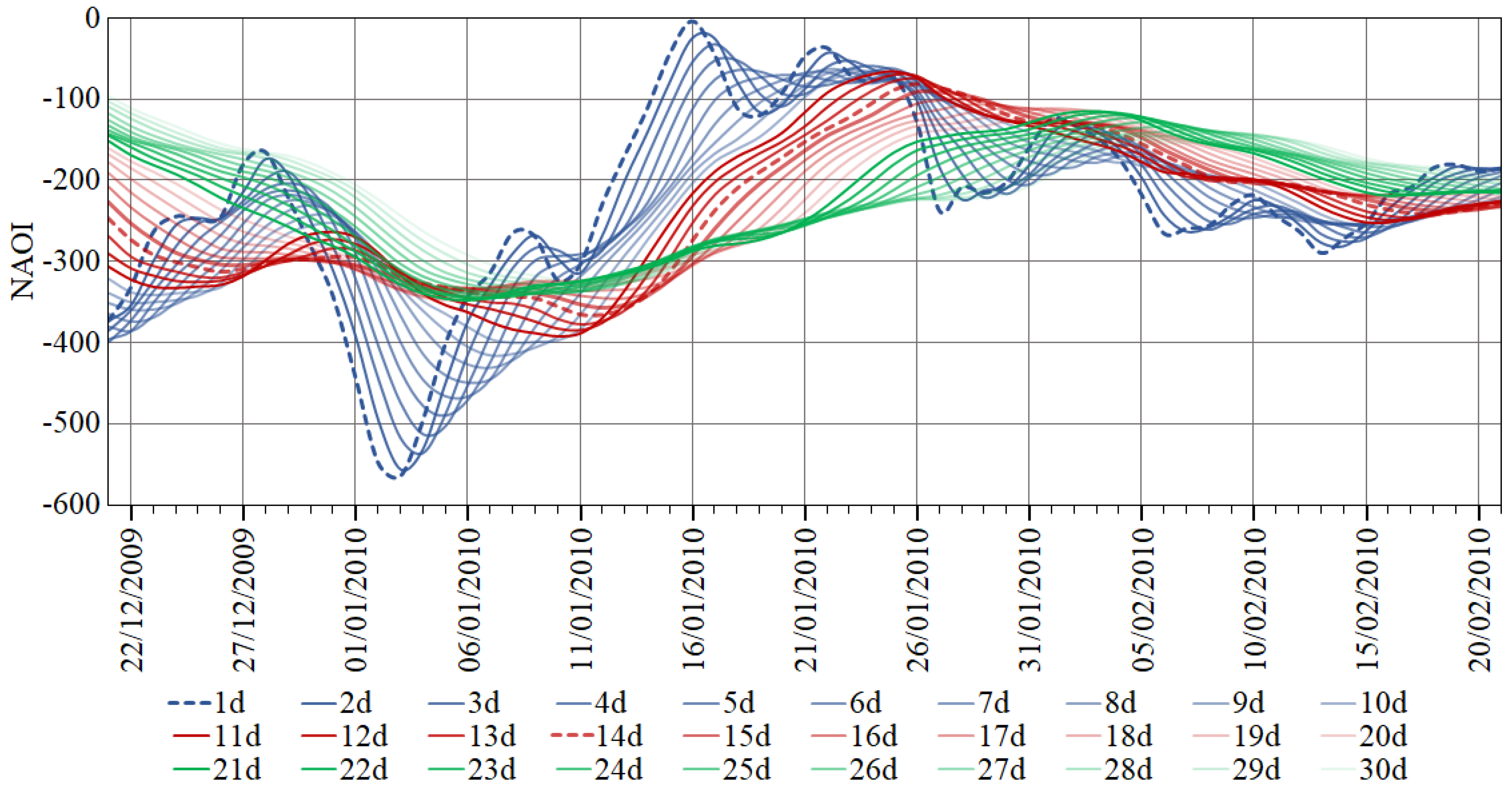
22]. The daily rainfall records of that event were assigned to 9:00 am of the next day. A preliminary analysis of the NAOI suggested that such event could be teleconnected to the persistence of strongly negative values in previous days.
Figure 3 exemplifies an extract of the non-smoothed (1d) and smoothed NAOI values—from 2 days (2d) to 30 days (30d), i.e., low-pass filter
m from 2 to 30, respectively—from December 2009 to February 2010. In the figure, consecutive negative NAOI values can be observed in the first days of January 2010.
As mentioned, the effect of smoothed previous NAOI values on extreme rainfall events was assessed for the candidate rain gauge of Areeiro (AR-C), aiming at developing a criterion to align the bivariate series, which was then applied to the other rain gauges. AR-C has almost complete historic daily data and some of the island’s heaviest rainfall records, such as those that triggered the “
aluviões” (debris flows) on 20 February 2010. This assessment ascertained an alignment or cause–effect between the
X (smoothed and lagged NAOI) and
Y (extreme rainfall) series by maximising the Pearson correlation applied to the 45 selected extreme rainfall events at AR-C (depicted in
Figure 2a). This made it possible to identify (i) the running length,
m, of the low-pass filter of daily NAOI records, and (ii) the lag in days,
l, between the end of the smoothed NAOI series and the extreme rainfalls that occurred after that end.
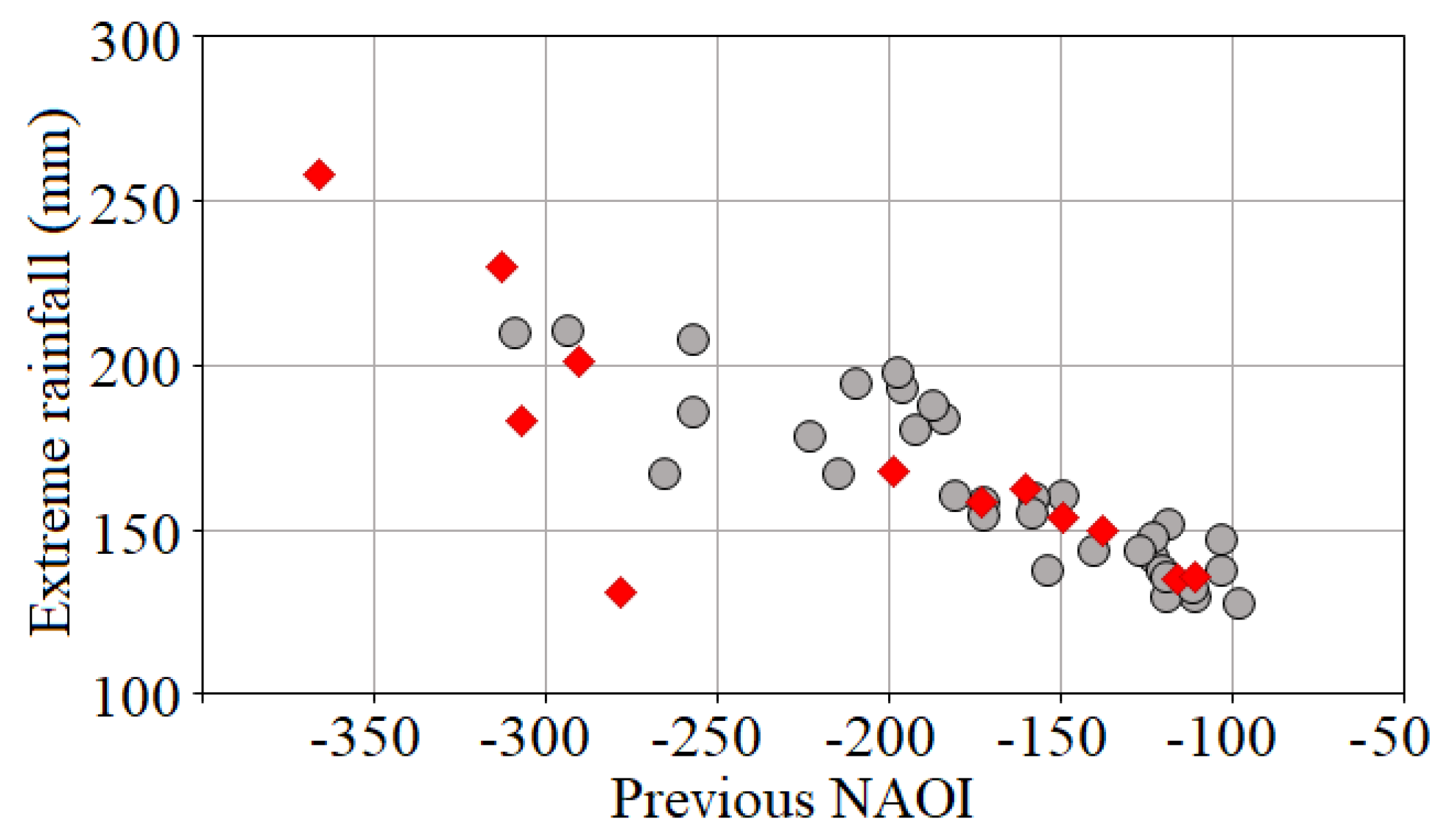
As a result of the previous analysis, a maximum value of
for the Pearson correlation coefficient was obtained based on the low-pass filter of
(14d) averaged NAOI values, ending 39 days prior to the extreme rainfalls events—depicted in
Figure 4. For
m values lower and higher than 14, but also for
l values shorter and longer than 39 days, the correlations between coupled NAOI values and extreme rainfalls yielded no statistically significant improvements.
In order to establish the final dataset for teleconnection via copulas, the same and l = 39 days for NAOI—hereafter referred to as previous NAOI values—were adopted at the other rain gauges, rather than repeating the analysis for each of them. The main purpose of this was to conclude on to what extent the results obtained based on AR-C could be adopted over the island, thus simplifying further analysis on the effect of the NAO persistence over the rainfall regime in Madeira. Albeit based on the same m and l, the previous NAOI values assigned to the extreme rainfalls may differ among rain gauges due to the different dates of occurrence of those events.
The copulas modelled in this research work corresponded to
all the variables being independent [
53]. This is the copula type of any random vector established by independent variables. The elements of the extreme rainfall series may, in practice, be assumed to be independent [
41]. In some cases, however, there may be significant dependence among extreme values even though they are random in a series. Conversely, independence implies that no observation in the data series has any influence on any following observations. In this regard, the independence of the univariate vectors of previous NAOI and extreme rainfalls was evaluated via the Wald–Wolfowitz runs test having the null hypothesis
of independence with 0.05 as the critical value. The null hypothesis was tested at the six stations, resulting in
p-values ranging from 0.31 to 0.97, for previous NAOI, and from 0.11 to 0.79, for extreme rainfall. As these results are greater than the critical value, it was not possible to reject the
of independence in any case.
4.3. Bivariate Joint Distributions and Constructed Copulas
Before showing the dependence modelling of the two random variables via copulas, the resulting descriptive statistics of the bivariate series are presented in
Table 3. As the values of the previous NAOI are always negative, in the copulas models,
refers to their opposites. Additionally, given that the number of extreme rainfalls events and of analysed years are the same for the six rain gauges, the resulting
E(
L) is also the same (0.90). The Kendall’s
correlation coefficient presents a high negative value for AR-C, which is in accordance with the visible dependence in the scatter plot set out in
Figure 4, and with the Pearson correlation (
r). Still, Kendall’s
measures only the overall strength of the association between previous NAOI and extreme rainfall, but does not provide accurate information about how this association varies across the distribution [
54]. The mean values of extreme rainfall suggest similar characteristics at the central highlands (AR-C and BC-C), with higher values than the lowlands (e.g., FO-S and PP-W), as previously identified (
Section 4.1). Concerning the mean of previous NAOI, values are homogeneous in the six series. Note that the most negative previous NAOI (min of
) always appears in the coupled series. Such a value resulted from consecutive strongly negative NAOI in the first days of January 2010 (
Figure 3) that was assigned to the rainfalls on 20 February 2010. The previous assessment is somewhat unclear since it is based on a univariate perspective that justifies a copula-based characterisation of the bivariate dependency structure.
The bivariate joint distributions between previous NAOI and extreme rainfall were determined to model copulas for teleconnection, aiming at obtaining the corresponding return periods. One copula function was selected for each rain gauge, as indicated in
Section 3.3.
Table 4 reports the selected copulas for the bivariate series based on the marginal distributions of previous NAOI and extreme rainfall. The estimated parameters and values of the goodness-of-fit test (AIC) for the best-fitted copulas and marginal distributions are listed in the same table. The selection of marginals for the individual variables (log-normal in most cases) allowed us to model the dependence structure via copulas. Only AR-C and SC-E have the same selected copula family, i.e., Survival Gumbel, whether different copulas were assigned to the other four rain gauges. This means that the joint bivariate characteristics and their dependences are distinct among the regions of the island and thus need specific copulas to be modelled.
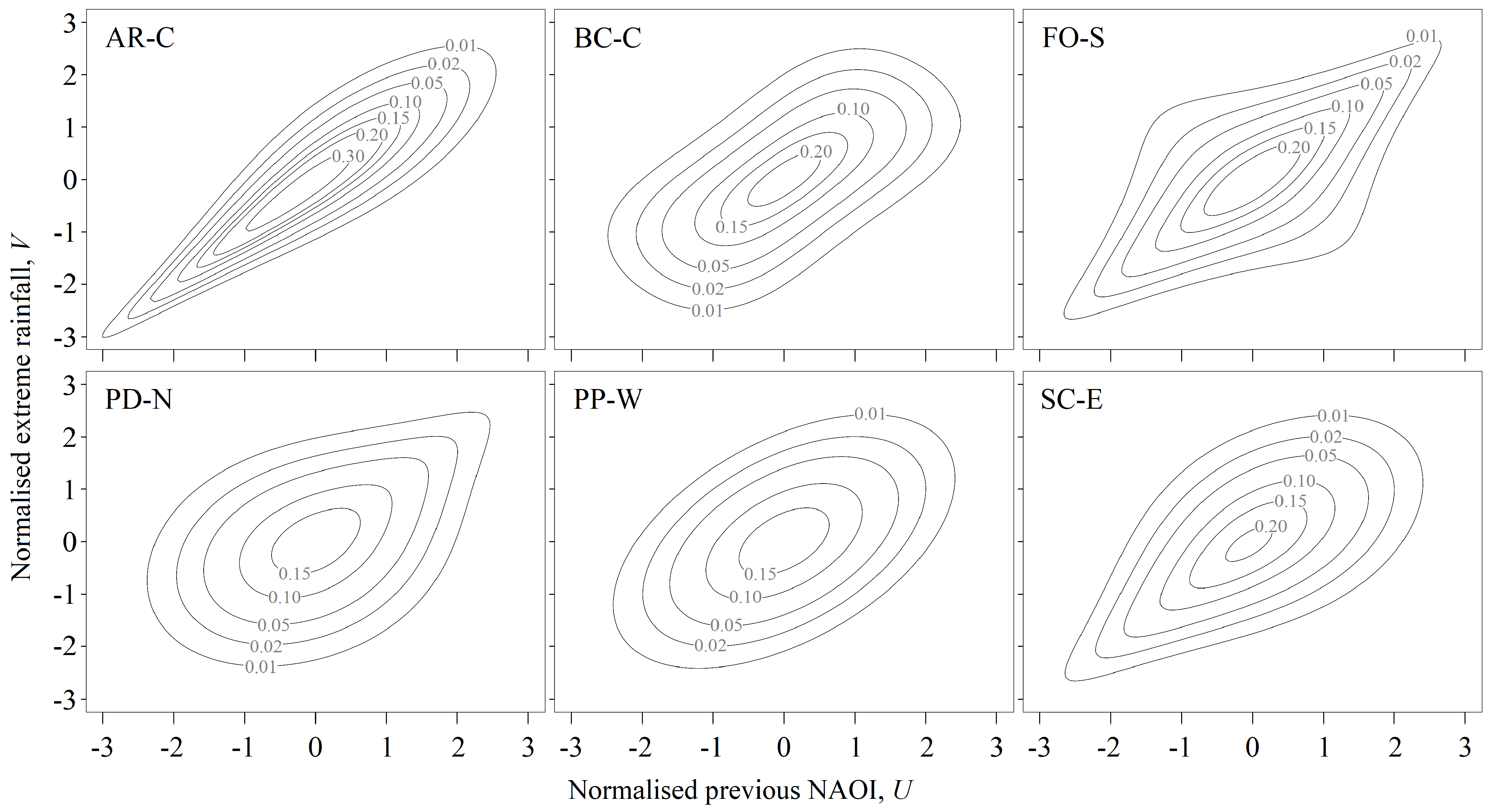
The copulas
that best describe the observed dependence patterns between normalised values of previous NAOI,
U, and of extreme rainfall,
V are presented as contour lines in
Figure 5. The normalisation of values was carried out to allow direct comparisons among the multivariate normal shapes of the rain gauge observations and bring out specific features, such as the dependence measure of tail dependence [
48]. This allowed us to determine the level of association among extreme events in the lower and upper tails for previous NAOI and extreme rainfall, respectively. In this case, the previous NAOI lower tail corresponds to strongly negative previous NAOI values and the importance of this association lies in the fact that negative NAOI values have been connected to impacts on regional climate variability during winter (e.g., [
55]).
Figure 5 shows that the Survival Gumbel copula (the rotated Gumbel copula) best-fitted the bivariate series at AR-C and SC-E rain gauges with a stronger dependency in the lower tail of previous NAOI and in the upper tail of extreme rainfall. On the other hand, the PD-N series presented a Gumbel copula with an inverted dependence structures. The copulas for FO-S and PP-W are of the same class, i.e., meta-elliptic copulas (
Table 2), although with different dependence structure. The joint distribution at FO-S was modelled with a Student’s
t copula by generating joint symmetric tail dependence, hence allowing an increased probability of joint extreme events. For the series at PP-W, the Gaussian copula was used by generating joint symmetric dependence, and, according to the copula’s characteristics, with no tail dependence, i.e., no joint extreme events. For BC-C, the goodness-of-fit test resulted in well-fitted Frank copula being symmetric and with more probability concentrated in the tails, but without lower or upper tail dependence. Rather than from just a linear correlation analysis, these results robustly evidence different dependence structures between previous NAOI and extreme rainfalls across the island.
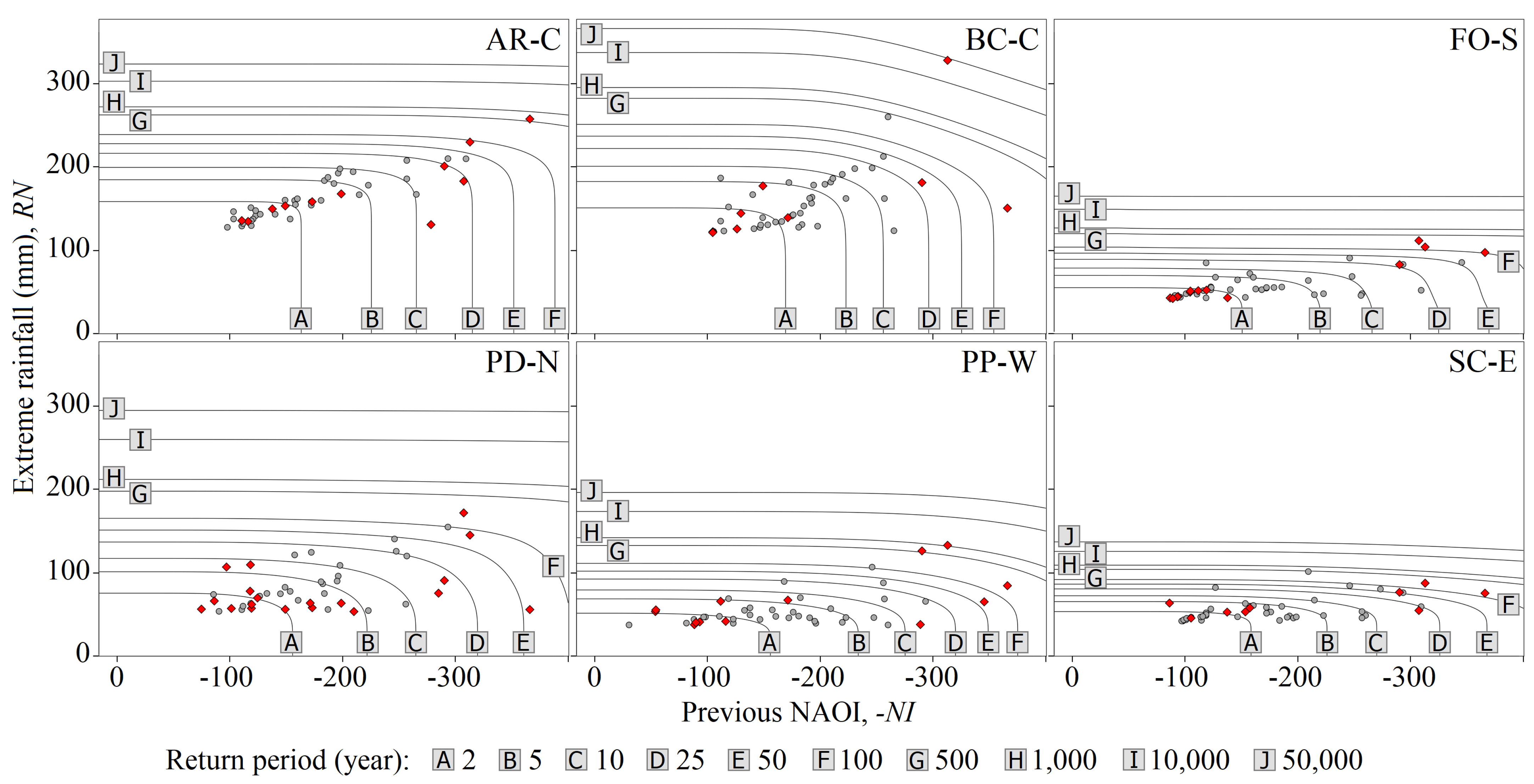
4.4. Bivariate Return Periods of the Previous NAOI and Extreme Rainfall Events
The return periods
, defined by Equation (
8), of the 45 coupled events depending upon the modelled joint behaviour of the two random variables at each rain gauge are shown in
Figure 6. Those with the highest return periods
are reported in
Table 5. Since various combinations of previous NAOI and extreme rainfall can result in the same
, the return periods are presented as contour lines in the figure. These lines are bounded by the axes and denote different patterns regarding the location of the rain gauge on the island. As an illustrative example, a combination of previous NAOI of
and a daily rainfall of 100 mm results in
years at the central highlands (AR-C and BC-C),
years on the southern lowland (FO-S),
years on the northern slope (PD-N),
years in the western area (PP-W), and
years in the eastern region of the island (SC-E).
Figure 6 also presents the bivariate events, differentiating those from the initial 33-year sub-period, from December 1967 to February 2000, to the ones from the final 17-year sub-period, from December 2000 to February 2017. For the initial sub-period, this differentiation resulted in 33, 36, 32, 26, 32, and 35 extreme events for AR-C, BC-C, FO-S, PD-N, PP-W, and SC-E, respectively, and consequently, for the final sub-period, in 12, 9, 13, 19, 13, and 10 events. By dividing the number of events by the number of years of their respective sub-periods, interarrival times different to the one used to construct copulas were obtained. A comparison of the
E(
L) between the two sub-periods revealed that for all the rain gauges, except for PD-N,
E(
L) decreased, meaning less frequent extreme rainfall events in the last 17 years. However, the figure shows that the most extreme bivariate events with higher return periods, except for SC-E, always took place in the more recent sub-period.
Figure 7 depicts the conditional return periods, i.e., the return period of extreme rainfall, given that the previous NAOI is lower than a certain threshold. Note that the horizontal axes are always the same but the vertical axes are not. Moreover, some of the more exceptional bivariate events of
Table 5 are not depicted in the figure due to the adopted vertical scales. For uniformity purposes, the reported events are those with the highest return periods associated with
, as previously mentioned. By way of example, for AR-C, regardless the return period approach, the most unusual event occurred in February 2010 with previous NAOI of −366.0 and extreme rainfall of 257.6 mm. The univariate analysis, based on the best-fitted marginal distribution and Equations (
6) and (
7), resulted in return periods of 491 and 2646 years, respectively. From the multivariate analysis, the joint return period (Equation (
8)) is 4407 years, whereas the conditional one (Equation (
9)) corresponds to 259,894 years.
In general terms, the achieved univariate and bivariate return periods from December 1967 to February 2017 show that the island has been characterised by numerous events with an unsteady chronological development, particularly with highly negative previous NAOI and more intense extreme rainfalls in earlier years. Based on the results shown in
Figure 6 coupled with those reported in
Table 5, from December 2010 to February 2011, the persistently negative phase of the NAO (in this case, previous NAOI) is according to the assumptions made for the bivariate problem in generating highly winter daily extreme rainfalls across Madeira. These observed extreme rainfall patterns can, however, be attributed—among other atmospheric processes—to the leading pattern of climate variability over the Northern Hemisphere, i.e., to the NAO variability.


 ,
, 


