
Assessing Impact of Climate Variability in Southwest Coastal Bangladesh Using Livelihood Vulnerability Index


1
South Asian Water (SAWA) Fellowship Program, Institute of Water and Flood Management, Bangladesh University of Engineering and Technology, Dhaka 1000, Bangladesh
2
Institute of Water and Flood Management, Bangladesh University of Engineering and Technology, Dhaka 1000, Bangladesh
*
Author to whom correspondence should be addressed.
Climate 2021, 9(7), 107; https://0-doi-org.brum.beds.ac.uk/10.3390/cli9070107
Submission received: 19 May 2021
/
Revised: 15 June 2021
/
Accepted: 24 June 2021
/
Published: 29 June 2021
(This article belongs to the Special Issue Sub-Regional Scale Climate Change)
Abstract
:This study analyzed the variability of rainfall and temperature in southwest coastal Bangladesh and assessed the impact of such variability on local livelihood in the last two decades. The variability analysis involved the use of coefficient of variation (CV), standardized precipitation anomaly (Z), and precipitation concentration index (PCI). Linear regression analysis was conducted to assess the trends, and a Mann–Kendall test was performed to detect the significance of the trends. The impact of climate variability was assessed by using a livelihood vulnerability index (LVI), which consisted of six livelihood components with several sub-components under each component. Primary data to construct the LVIs were collected through a semi-structed questionnaire survey of 132 households in a coastal polder. The survey data were triangulated and supplemented with qualitative data from focused group discussions and key informant interviews. The results showed significant rises in temperature in southwest coastal Bangladesh. Though there were no discernable trends in annual and seasonal rainfalls, the anomalies increased in the dry season. The annual PCI and Z were found to capture the climate variability better than the currently used mean monthly standard deviation. The comparison of the LVIs of the present decade with the past indicated that the livelihood vulnerability, particularly in the water component, had increased in the coastal polder due to the increases in natural hazards and climate variability. The index-based vulnerability analysis conducted in this study can be adapted for livelihood vulnerability assessment in deltaic coastal areas of Asia and Africa.
1. Introduction
Bangladesh lies at the bottom of the Ganges–Brahmaputra–Meghna river basin, which is the largest river basin in the world [1]. The country is watered by a total of 57 transboundary rivers, 54 originating from neighboring India and three from Myanmar. The geographical location of Bangladesh and its geomorphic conditions have made the country highly vulnerable to climate variability, climate change, and natural disasters [2]. Coupled with widespread poverty and high population density, the limited adaptive capacity and poorly funded, ineffective local governance have made the country one of the most adversely affected countries on the planet. Indeed, Bangladesh has been among the 7th most affected countries in the last two decades (1999–2018) according to the Global Climate Risk Index 2020 [3]. Among all the areas of Bangladesh, the coastal area is the most vulnerable and hazard-prone to climate variability and change.
The coastal areas of Bangladesh are different from the rest of the country, not only because of their unique geophysical characteristics, but also for different sociopolitical consequences that often limit people’s access to endowed resources and perpetuate risks and vulnerabilities [4]. For coastal communities, agriculture is the most dominant livelihoods and a major driver of socio-economic development [5]. However, the impacts of climate variability and change, such as heightened damage due to storm surge, progressive inundation from sea level rise, and increased salinity from saltwater intrusion, are hampering the agriculture-dependent livelihood.
Several studies were conducted on climatic trends and climate change impacts in the coastal region of Bangladesh [6,7,8,9,10,11,12,13]. A qualitative assessment of climate change impacts on livelihood in the southwestern coastal zone of Bangladesh was done using secondary data and information in [11]. Water shortages for agriculture, water logging, and storm surge flooding were identified as the major factors affecting livelihoods. Vulnerability of climate change affected communities in a sub-district of southwestern coastal zone of Bangladesh was assessed using a socioeconomic vulnerability index (SeVI) in [8]. SeVI consisted of three dimensions (adaptive capacity, sensitivity, and exposure) and five domains (demographic, social, economic, physical and exposure to natural hazards). Livelihood vulnerability in the 137 polders of Bangladesh was also assessed from survey-based interviews, secondary information and geo-spatial analysis using a sustainable livelihood approach in [12]. However, the impacts of natural disasters, climate change, and climate variability were not included in the vulnerability equations. In a recent study [13], livelihood vulnerability in four polders for three-time horizons (current, response and onset of polderization) was assessed using livelihood vulnerability index (). The study found that the livelihood vulnerability of communities living in all four polders had reduced in the current period compared to the response and onset periods. However, it is not understood how reliable the responses of the interviewees with age of 30–55 years would be for events that happened 50–60 years back (polder onset period in 1960s).
In none of the above studies in Bangladesh, climate variability and its impact on local livelihood were studied. There was a study on rainfall variability [14] and another study on local perception of and adaptation to climate variability and change [15]. Clearly, there is a research gap in Bangladesh regarding climate variability and its impact, though such researches were conducted in a number of other countries (e.g., at two districts in Mozambique [16], for two wetland communities in Trinidad and Tobago [17], among smallholder horticultural farming households in two districts in Ghana [18], for smallholder farmers in northern Ghana [19], for three agricultural and natural resource dependent commune in northwest Vietnam [20], for two regions in Uttarakhand, India [21], for mixed agro-livestock smallholders in three ecological zones in the Gandaki River Basin of central Nepal [22]). Climate change is a long-term process, so its effects become visible gradually with time. While the climate tends to change quite slowly, that does not mean that we do not experience short-term fluctuation at seasonal or multi-seasonal time scale. A climatic parameter can fluctuate around its average without causing the long-term average itself to change. This phenomenon is the climate variability [23]. According to the Intergovernmental Panel on Climate Change, climate variability is the variations in the mean state and other statistics, such as standard deviation and extremes, of climate at all temporal and spatial scales beyond that of individual weather events [24]. Simply put, climate variability describes the way climate elements, such as temperature and rainfall, depart from their average values in given months, seasons, years, decades, or centuries.
The main objectives of this study were to assess the variability and trend in important climatic parameters, such as rainfall and temperature, in the southwest coastal Bangladesh, and to assess the impacts of such climate variability on local livelihoods using livelihood vulnerability index (). The specific research question that the study sought to answer was: What was the direction of climate variability so far in the sub-region, and how was that affecting different components of local livelihood? The assessment of climate variability and trend would help better understand the present climatic hazards in the study area. The index-based evaluation of its impacts on local livelihoods would help policy makers and relevant local and national organizations towards modification of existing adaptation strategies and development of new strategies. The interdisciplinary approach and methodology followed in this study, and the techniques and tools used, have the potential to be applied elsewhere in deltaic coastal setting of Asia and Africa for livelihood vulnerability assessment.
2. Materials and Methods
2.1. Study Area
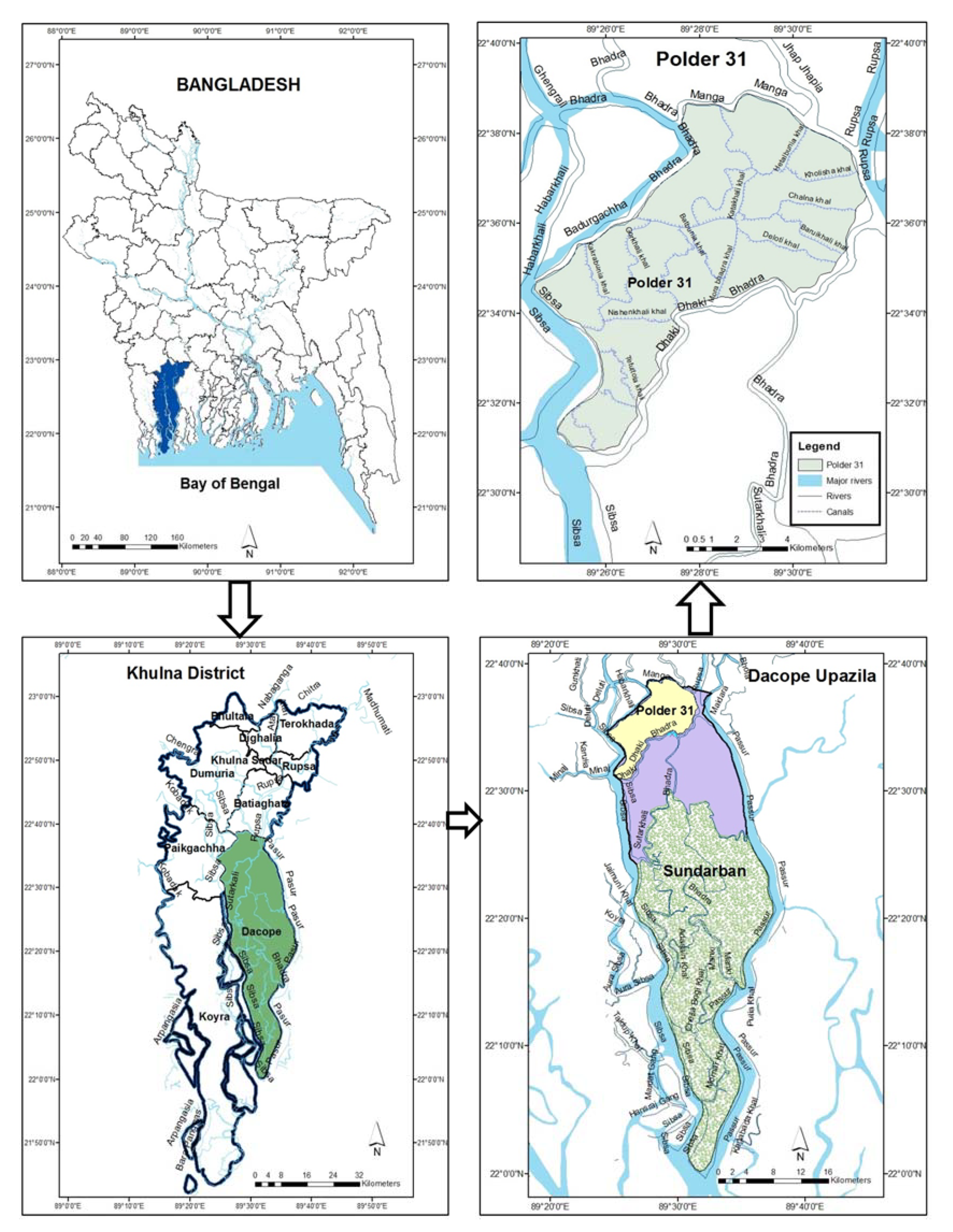
The study was conducted in Khulna district, which is situated in the southwest coastal region of Bangladesh (Figure 1). The district consists of nine upazilas (sub-districts), and Dacope is the second largest upazila after Koyra. The upazila faces the common natural hazards of coastal Bangladesh, such as cyclone, storm surge, salinity intrusion, river and coastal erosion, water logging, and seasonal flood, and represents the typical geophysical and socioeconomic settings of sea-facing southwest coastal Bangladesh. The upazila consists of three different polders, namely polders 31, 32, and 33. Among these, Polder 31 faces the negative impacts of climate variability and change more than the other two [25], and hence it was selected for this study. Untimely rain, unusual heavy rainfall, high temperature, prolonged drought, and other natural disasters had been disrupting the local livelihoods in the upazila for the last few decades.
2.2. Analysis of Climate Variability
Several techniques were employed for the analysis of rainfall and temperature data, which generally fall into variability and trend analysis. Variability analysis involved the use of coefficient of variation (CV), mean standardized anomaly (Z), and precipitation concentration index (PCI) [26]. Though different indices are available to examine variability/heterogeneity in rainfall pattern and to analyze and understand hydro-meteorological processes, PCI was recommended in [27] as it provides information on long-term total variability in the amount of rainfall received [28,29,30]. Different ranges of PCI denote different concentrations of rainfall. Hence, was included to examine the variability in rainfall at different temporal scales (annual or seasonal). Calculations were carried out using the Statistical Package for Social Sciences (SPSS) version 25 software.
Trend analysis was performed through the Mann–Kendall (MK) trend test. The MK test is a non-parametric test, which tests for a trend in a time series without specifying whether the trend is linear or non-linear [31]. The advantage of the non-parametric statistical test over the parametric test is that the former is more suitable for non-normally distributed, censored, and missing data with outliers and extremes, which are frequently encountered in climatic time series. As a result, the MK test is widely used to detect trends of meteorological parameters [26].
CV was calculated to evaluate the variability in the annual, seasonal and monthly rainfalls. CV was computed as:
where, σ is the standard deviation and μ is the mean of rainfall. A higher value of CV indicated a larger variability, and a lower value a smaller variability. CV was used to classify the degree of variability of rainfall events as less (CV < 20), moderate (20 < CV < 30), and high (CV > 30) [32].
PCI was computed as [27]:
where is the rainfall amount in the th month and is the number of months in a year or season. PCI can be calculated at seasonal scale [30], and hence dividing the year into two seasons, i.e., dry season (November–May) and monsoon season (June–October), the PCI values at seasonal scale were calculated. A PCI value of less than 10 indicated a uniform monthly distribution of rainfall (low precipitation concentration), a value between 11 and 15 indicated a moderate concentration, a value from 16 to 20 indicated a high concentration, and a value of 21 and above indicated a very high concentration [27].
The rainfall determined for each year can be used to understand the nature of variability, to determine the dry and wet years in the record, and to assess the frequency and severity of drought [33,34,35]. Z was calculated as:
where is the annual rainfall of a particular year, is the long-term average annual rainfall over a period of observation and is the standard deviation of the annual rainfall over the period of observation. The drought severity classes were extreme drought ( < −1.65), severe drought (−1.65 < < −1.28), moderate drought (−1.28 < < −0.84), and no drought ( > −0.84) [36].
Trend analysis was conducted for both temperature and rainfall at annual as well as seasonal (dry and monsoon seasons) scales. The MK test statistic was calculated as [31,37,38]:
where and are the annual values in years and , respectively. The test required the sample data to be serially arranged. Thus, the time series was serially arranged from and from . Each of the data points was taken as a reference point, which was then compared with the rest of the data points so that:
when the number of observations is 10 or more ( ≥ 10), the statistic is approximately normally distributed with its mean , which becomes 0 [38]. In this case, the variance of is given by:
where is the number of groups with tied ranks, each with tied observations. The test statistic is as follows:
The above statistic was used to identify the increasing or decreasing trend in the time series of climatic parameters. A positive indicated an upward trend and a negative a downward trend in the time series. Since is approximately normally distributed, the p-value could also be computed from the value to find the significance level of the trend. If the p-value was small enough, the trend was quite unlikely to be caused by random sampling.
2.3. Assessment of Impact of Climate Variability
Impact of climate variability on livelihood was assessed by developing a livelihood vulnerability index (). Such index was also used to identify and compare climate change-specific livelihood vulnerabilities [16,17]. The extent of the impacts of climate variability and change on livelihood depends on the level of vulnerability of farmers and people of other occupations to these impacts [19]. Livelihood becomes more vulnerable if climate variability impacts more negatively. The index value ranges from 0 to 1, 1 being the highest vulnerability.
The included six major components: socio-demographic profile (), livelihood strategies (), health (), food (), water (), and natural disasters and climate variability () [16]. Each component was comprised of several sub-components or indicators. These were developed based on a review of relevant literature on each major component and considering local socioeconomic and biophysical contexts. Table 1 provides an explanation of how each sub-component was quantified, the survey question was used to collect the data, and what the original source of the survey question was.
The s were developed for the last two decades (1998–2007 and 2008–2017) and compared to estimate the differential impacts of climate variability in the two consecutive decades. Difference in values between the two decades indicated whether the vulnerability had increased, or not, in the present decade (2008–2017) compared to the past (1998–2007) due to climate variability. Since the development of was dependent on primary data collected through questionnaire survey, the generation of for any earlier decade was not possible as most people could not look back to a very old time or recall an old event. People were able to talk fluently about events and impacts that happened in the last 20 years. Though some senior people could provide information on some distant-past events, those could not be triangulated from other sources.
A balanced weighted average approach was followed to construct the where each sub-component had equal contribution to the overall index even though each major component was comprised of a different number of sub-components [16,39]. As we intended to develop an assessment tool accessible to a diverse set of users in resource-poor settings, the procedure needed to be simplified and hence the formula used the simple approach of applying equal weights to all sub-components. This weighting scheme can be adjusted by future users if needed.
Because each sub-component was measured on a different scale, it was necessary firstly to standardize the sub-component value as an index:
where is the original value of a sub-component for a decade, and and are the minimum and maximum values, respectively, for the sub-component determined using the data from both the decades.
For the sub-components that measured frequencies, such as the ‘percentage of households that reported conflicts over water resources in their community or village’, the minimum value was set at 0 and the maximum at 100. Some sub-components, such as the ‘average agricultural livelihood diversity index’, were created such that an increase in the crude indicator, in this case, the number of livelihood activities undertaken by a household, would decrease the vulnerability. In other words, we assumed that a household who farmed and raised animals was less vulnerable than a household who only farmed. By taking the inverse of the crude indicator, we created a number that imparted a higher value to the household with a lower number of livelihood activities. The maximum and minimum values were also transformed following this logic and Equation (8) was used to standardize these sub-components.
After standardization of each sub-component, the average of the sub-components under each major component was calculated to obtain the respective major component value :
where, is the number of sub-components under the given major component.
Once the values of the six major components for a decade were calculated, these were averaged to obtain the for the decade:
where is the for the decade , and equals to the weighted average of the six major components. represents the weights of the sub-components that make up each major component. As mentioned earlier, the weight of each major component was determined by the number of sub-components that made up each major component. The ranged from 0 (least vulnerable) to 1 (most vulnerable).

Table 1.
Major components and sub-components of LVI.
| Major Component | Sub-Component | Explanation of Sub-Component | Survey Question | Source of Question |
|---|---|---|---|---|
| SDP | Dependency ratio | Ratio of the population under 15 and over 65 years of age to the population between 15 and 64 years of age. | Could you please tell the ages and sexes of every person who eats and sleeps in this house? If you had a visitor who ate and slept here for the last 3 days, please include them. | Adapted from [40] |
| Head of household not attending school | Percent of households where the heads reported that they have attended 0 years of school. | Did you ever go to school? | Adapted from [40] | |
| LS | Household with family member working outside | Percent of households that reported at least 1 family member working outside the community for their primary work activity. | How many people in your family went to a different community to work? | Adapted from [41] |
| Household depending solely on agriculture | Percent of households that reported only agriculture as a source of income. | Did your household depend on income only from raising animals, growing crops, or collecting and selling something from the forests, wetlands, or rivers? | Adapted from [41] | |
| Average agricultural livelihood diversification index (range: 0.20–1) | The inverse of (the number of agricultural livelihood activities +1) reported by a household, e.g., a household that farms, raises animals, and collects natural resources has a livelihood diversification index = 1/(3 + 1) = 0.25. | Same as above. | Adapted from [40] | |
| H | Household with family member chronically ill | Percent of households that reported at least 1 family member with chronic illness. | Was anybody in your family chronically ill (they got sick very often)? | Adapted from [40] |
| Household with family member missing work/school | Percent of households that report at least 1 family member who had to miss school or work due to illness in the last 2 weeks. | Was anyone in your family so sick in the past 2 weeks that they had to miss work or school? | Adapted from [41,42] | |
| F | Household depending on family farm for food | Percent of households that get their food primarily from their own farms. | Where did your family get most of its food? | Developed by the authors |
| No. of months households struggling to find food | Percent of households that get their food primarily from their own farms. | Did your family have adequate food for the whole year, or were there times when your family did not have enough food? How many months a year did your family have trouble in getting enough food? | Adapted from [41] | |
| Average crop diversity index | The inverse of (the number of crops grown by a household +1). | What kind of crops did your household grow? | Adapted from [41] | |
| Household not saving crops | Percent of households that do not save crops from each harvest. | Did your family save some of the crops that you harvested to eat during a different time of the year? | Authors | |
| Household not saving seeds | Percent of households that do not have seeds from year to year. | Did your family save seeds to grow in the next year? | Authors | |
| W | Household using natural source for domestic water | Percent of households reporting a tube well, dug well, river, or pond as primary water source. | Where did you collect your water from? | Adapted from [40] |
| Household reporting water conflict | Percent of households that report suffering from or having heard about conflicts over water in their community. | In the past years, did you hear about any conflict over water in your community? | Adapted from [40] | |
| Household without consistent water supply | Percent of households that report that water is not available at their primary water source or delivered to them every day. | Was this water available every day or regularly? | Adapted from [41] | |
| NDCV | No. of natural hazard events in the past 20 years | Total number of floods, droughts and cyclones reported by households in the past 20 years. | How many times were this area affected by a flood/cyclone/drought during past 20 years? | Adapted from [43] |
| Household not receiving a disaster warning | Percent of households that did not receive a warning of severe flood, drought, and cyclone events in the past 20 years. | Did you receive a warning about the flood/cyclone/drought before it happened? | Adapted from [43] | |
| Monthly standard deviation of maximum temperature | BMD data | Standard deviation of the average daily maximum temperature by month between 1998 and 2017 averaged for each decade. | Adapted from [44] | |
| Monthly standard deviation of minimum temperature | BMD data | Standard deviation of the average daily minimum temperature by month between 1998 and 2017 averaged for each decade. | Adapted from [44] | |
| Monthly standard deviation of rainfall | BMD data | Standard deviation of the average monthly rainfall between 1998 and 2017 averaged for each decade. | Adapted from [44] |
2.4. Data Collection
For climate variability analysis, daily data on maximum and minimum temperatures and rainfall at the Khulna station of the Bangladesh Meteorological Department (BMD) were collected from the BMD for the period of 1978–2017. For livelihood vulnerability assessment, primary data were collected from a household-level survey in Polder 31 using a pre-tested, semi-structured questionnaire. The questionnaire was framed such that all the sub-components, which eventually composed the major component, were adequately captured. A face-to-face interview was conducted to administer the questionnaires among 132 households of the polder. Sample households were selected based on a stratified purposive sampling technique and included farmers, fishermen, local businessmen and women. The geographic distribution of households, representativeness of local livelihoods, and availability of survey resources guided the selection of respondents and the sample size. To compare our sample size of 132 in one polder, 162 respondents were surveyed in four polders in [13], 50 households in [21], and 171–192 households per district in [22]. For triangulation of the survey data and to supplement and complement the study findings, qualitative field data were also collected using several participatory tools, such as key informant interviews (KIIs), Focus Group Discussions (FGDs), case studies and transect walks. The key informants included local officials, public representatives, and civil society personnel. The FGDs were conducted with the farmer, fisherman, and woman groups. The field data were collected in the years of 2018 and 2019 through a number of field visits to the study area.
3. Results and Discussion
3.1. Climate Variability in Southwest Coastal Bangladesh
3.1.1. Temperature
Analysis of annual, seasonal, and monthly temperatures was performed to detect the variability and trend in temperature in the study area for the period of 1978–2017. Linear regression models were fitted to the monthly and seasonal average temperatures, and also to the annual maximum, minimum, and average temperatures. The goodness of fit of the regression model to a particular dataset was indicated by the coefficient of determination (R2) of the model, and the rate of change in temperature was indicated by the slope of the regression line.
The analyses revealed that the monthly (except for January) and seasonal (dry and monsoon seasons) average temperatures had a notable increasing trend in southwest coastal Bangladesh over the study period. Among the different months, July had the highest R2 value of 0.40 and November had the lowest value of 0.002. In the case of seasonal temperature, the monsoon season showed a notable increasing trend with R2 value of 0.52.
To know the significance of the trends, the MK test was done on the monthly, seasonal and annual temperatures. The test was applied on the maximum (Tmax), minimum (Tmin), and average (Tavg) temperatures for all the intra-annual data. Table 2 shows the MK significance levels along with the correlation coefficients obtained from the analysis. As seen in the table, the maximum, minimum and average annual temperatures were increasing with time at nearly 1% significance level. May, June, July, August, and September showed upward trends in maximum and average temperatures at 1% significance level. The most significant increasing trend was found in the average temperature of the monsoon season with a p-value of 0.00031%. The maximum and minimum temperatures of this season also showed rising trends at 1% and 5% significance levels, respectively. January and November showed non-significant trends in all the temperatures. However, in most of the cases, the temperatures were increasing with time. Overall, there was a significant rise in temperature in the study area over the past four decades.
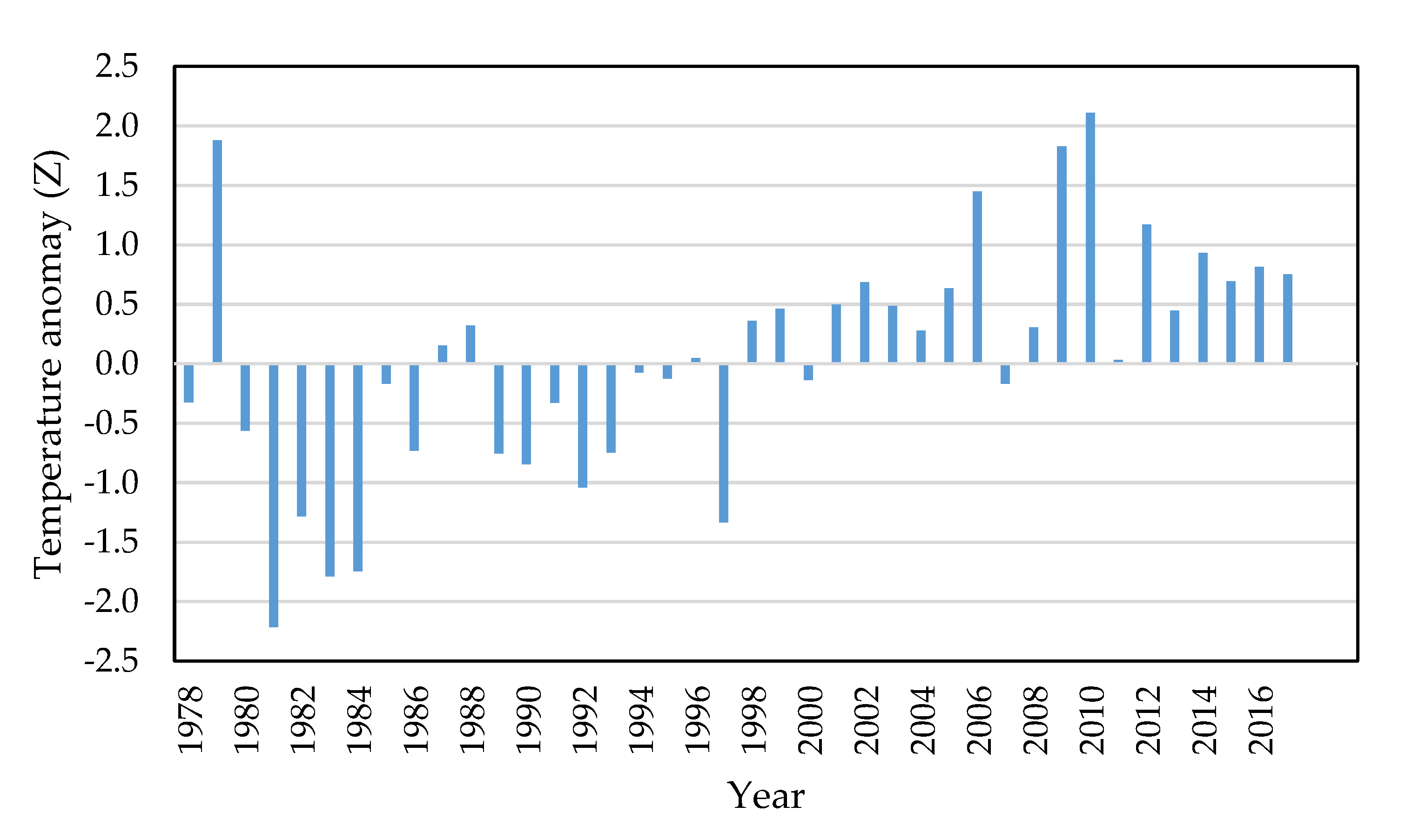
Variabilities in annual and seasonal mean temperatures were assessed by plotting the values against time (Figure 2 and Figure 3). The figures indicate how much variability each year had encountered during the past 40 years. In the case of annual temperature, earlier years showed the highest variability, then it decreased a little, but in recent years (1997, 2006, 2009, and 2010) a notable variability was recorded. Though the temperature variation in the dry season indicated a decrease in variability in the recent years, the variation in the monsoon season showed an increase in variability since 2009. The overall results indicated that there was a significant rise in temperature variability with time in southwest coastal Bangladesh.
3.1.2. Rainfall
Like temperature, the trend and variability analyses were done for rainfall of the study area over the period of 1978–2017. In addition to , the rainfall variability was investigated by other parameters like and .
Linear regression models (not shown) depicted increasing trends in rainfalls for July, September, and October as well as for the monsoon season, although the R2 values were very small. For February, March, April, June, and December, and also for the dry season, the models demonstrated slight declining trends over time. The linear regression lines (not shown) remained almost flat for January, May, August, and November indicating no change in rainfall in these months over the study period.
The correlation coefficients and MK significance levels are shown in Table 3. The table also includes CV, which measures the degree of variability in rainfall. It is seen from the table that July had an increasing trend and December had a decreasing trend at the 10% significance level. In both cases, the degree of variability in rainfall was high. Moreover, April had a decreasing trend, and August and the monsoon season had increasing trends at 20% level of significance. The monsoon season had a moderate degree of variability in rainfall, and annually, the degree of variability in rainfall was less. The other months showed a non-significant rising or falling trend in rainfall over the study period. These trends (Table 3) are consistent with the trends given in [14] as the latter reported an increasing trend in the monsoon rain and a decreasing trend in the pre-monsoon (March–May) rain at Khulna during 1958–2007.
The variability in rainfall was also analyzed by calculating separately for two seasons and plotting them against time (Figure 4). The result indicated that the variability in rainfall in the dry season was less than that of the monsoon season over the last 20 years. For the dry season, a higher variability was noted in 2009, 2010, 2011, 2014, and 2016, meaning that the years of the recent decade had witnessed a higher variability in comparison with the years of the past decade. A similar result was also found for the monsoon season, where the recent years (2007, 2012, and 2017) clearly demonstrated more variability than the past years.
was calculated for the past 40 years and the results are given in Table 4. The values indicate that the years of 1979, 1984, 2006, 2009, 2011, 2014, and 2015 had very high rainfall concentrations having PCI values of 21.50, 21.92, 20.44, 20.08, 21.84, 22.41, and 22.35, respectively. Thus, there were more recurring events of high concentration of rainfall in the recent decade than the past. Indeed, the average PCI values were found to be 18.68 and 16.66 for the present and past decades, respectively. Clearly, the PCI for the recent decade was higher than the past, indicating more variability in rainfall pattern at present. Moreover, as indicated by the PCI values, the variability in rainfall was mostly very high in the case of dry season, whereas it was mostly low and low to moderate in the case of monsoon season. In the dry season, the rainfall variability was very high in six years in both present and past decades. In the monsoon season, the variability was moderate in three years in the present decade compared to only one year in the past decade. So, from the overall results, it can be said that the variability or heterogeneity of rainfall in the study area had increased with time.
The values indicated that the years of 1985, 1989, 1996, and 2010 suffered from severe droughts (the values are −1.54, −1.36, −1.15, and −1.49, respectively), whereas the years of 1992 and 1994 witnessed extreme droughts. The average value for the present decade (2008–2017) was 0.03 compared to the value of 0.25 for the past decade (1998–2007). Thus, if we particularly focus on the last two decades, droughts were more pronounced in the present decade than the past decade as almost all the years of the past decade had seen ‘no drought’ events, but 2010 and 2014 encountered severe and moderate droughts, respectively.
3.2. Impact of Climate Variability on Local Livelihoods
Qualitative impacts of climate variability on various aspects of people’s livelihoods were known from the focused group discussions with the local people and key informant interviews. They informed that heavy rainfall, shifting of the monsoon and untimely rain were observed frequently in the recent years. The monsoon starting time, which was usually in early June, had changed for the last 10–12 years. A delayed onset of the monsoon and its increased unpredictability were noticed by the local people, which resulted in a delayed transplanting of the Aman rice with a consequent delayed harvesting and ultimately a yield loss. The local people found that the dry season became warmer, the temperature increased throughout the year and the warm summer period became longer. The bright sunshine hours had reduced, which hampered the post-harvesting activities of the crops. Pest infestation to crops had increased, growth period had shortened, and thus yield had decreased. Intrusion of salt water had reduced the yield of the Aman rice and had also reduced the cropping intensity. A description of increased climate uncertainty for dry season crop cultivation provided by a local farmer is given in Box 1 below without changing any detail:
Box 1. Uncertainty in dry season crop cultivation.
Mr. Rahmatullah, an informant from the study area (age 54, father of 4 children), shared his experience regarding the uncertainty in the dry season rainfall and temperature and its impact on his farming.
“I have been living in this village from my grandfather’s time, and farming is our only occupation. I have been cultivating sesame, pulses, watermelon and maize in the dry season for the last 25 years. As I remember, I rarely saw rains in the dry/winter season in the past. But for the last 4 to 5 years, sudden heavy shower of rain has been occurring along with more thunderstorms and cyclonic storms. Also, temperature is very high nowadays. Sometimes, we have to take showers even for 3 to 4 times a day and sit outside home in the hope of cold wind. Sudden rainfall and higher temperature are hampering our rabi crop cultivation. This unexpected rainfall sometimes causes waterlogging. In February of the last year, there was a sudden rain for 3 days at a stretch. The rainwater could not drain out immediately, so there was an instant waterlogging, and a large number of watermelons were destroyed as watermelon is intolerable to waterlogging.”
The local farmers faced a large impediment while cultivating their lands, as a thick layer of salt was deposited on the soil surface in the dry season. In addition, a higher frequency and intensity of storm surges and cyclones caused substantial losses to their standing crops. Disease outbreak/mortality in shrimp farms due to increased summer temperature, and soil and water salinity in croplands due to higher evaporation were also noticed. Stocking of freshwater fish was delayed due to the late onset of the monsoon season. These local perceptions on climate variability were consistent with the findings from secondary data in that both indicated rising temperature and increasing variability in temperature and rainfall.
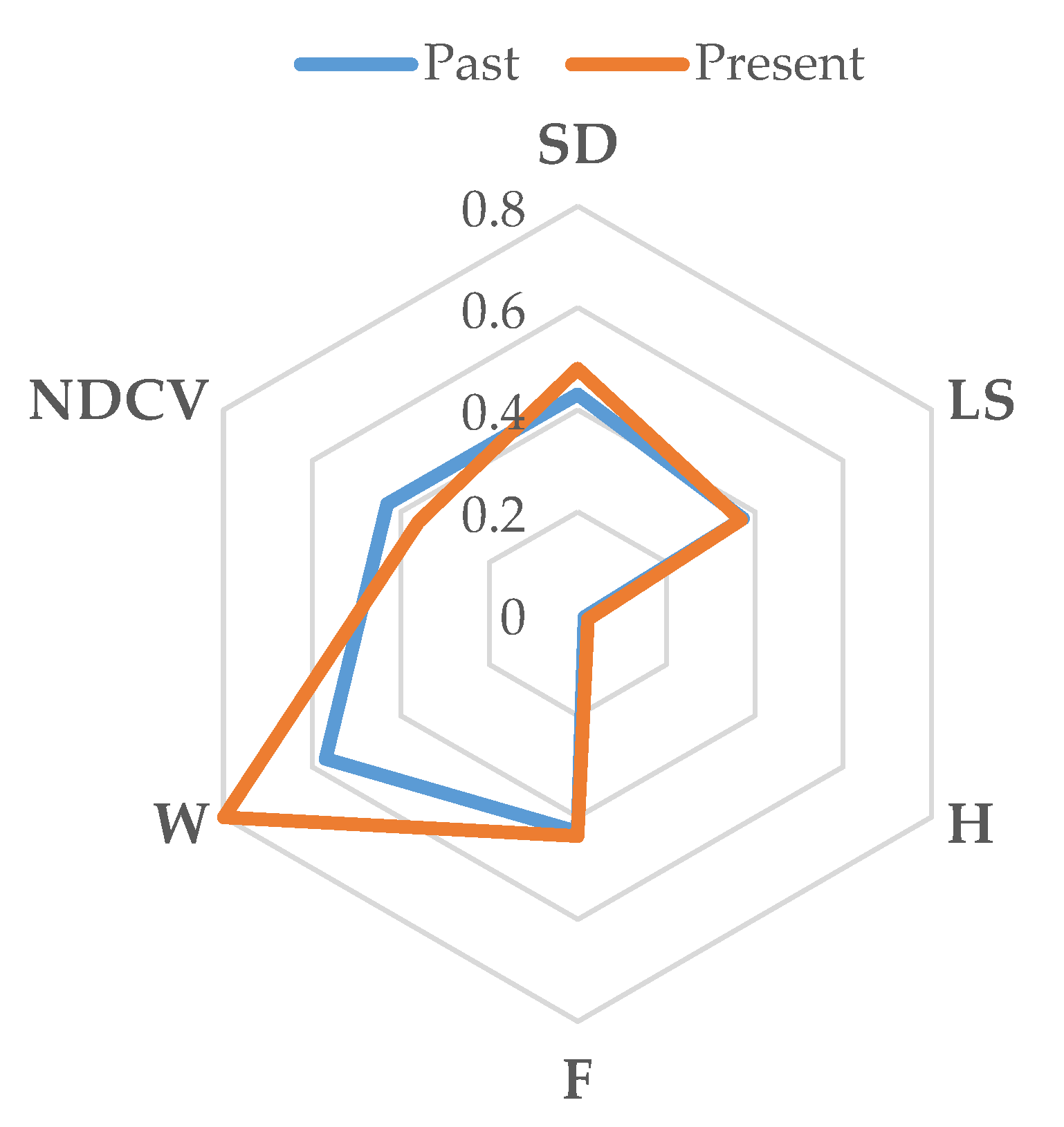
While the above narratives by the local people from their lived experiences provided a qualitative picture of their vulnerability to climate variability, a quantification of the impacts was also necessary to better understand the actual vulnerability. To quantify the impacts, was calculated for Polder 31 using Equation (10), and the results are presented in Table 5. The s for the past and present decades in the table were calculated based on major component values in Table 6 and Table 7. A visual representation of the major component values of the past and present s is shown in Figure 5 for an easy comparison. Overall, the present decade had a higher LVI than the past, indicating a relatively greater vulnerability of livelihood to climate variability and change impacts in the present decade.
4. Discussion
The first major component of is the (Table 5), which had increased in the present decade. This increase was due to the increases in both dependency ratio and illiteracy. The survey data revealed that there was an increase in the new children and older people among the surveyed households. In most cases, these children and older people could not contribute to the family income, so they became the dependent members of a family. Moreover, it was found that the percentage of household heads not attending school had actually increased.
Livelihood condition had slightly improved in the present decade than that of the past in terms of . In the recent decade, more people of the polder depended less solely on the income from agriculture. In addition, agricultural livelihood diversity, which means earning by the cultivation of different types of crops, had increased in the polder. That is why, the dependency on one or two crops had reduced significantly and most of the farmers started cultivating several crops round the year and were also adapting to mixed and cash crop cultivation nowadays. Salt and temperature tolerant high yielding varieties of rice were introduced to the farmers by the Department of Agriculture Extension for the purpose of adaption to the changing hydrology and climate in the coastal area [45]. However, more people had to work in a different community to earn their living in the present decade (20%) compared to the past (10%).
The most vulnerable sector due to climate variability and change was found to be the water sector. Households reported pond, river, rain, aquifer and dug well as their primary sources of water, and they used these sources for drinking, cooking, cleaning, washing, feeding cattle, and irrigating crops. Though the presence of salt, as well as iron, in most sources of water was quite common and higher in the present decade than that was before, people kept using these sources as they were abundant and easy to access. Previously, there were more freshwater sources, but recently, because of the increase in salinity, the options had reduced to a great extent. So, other than rainwater, only a handful of freshwater ponds were available to use. As groundwater was contaminated by salt, many tube wells became non-operational.
Water conflicts had increased from the previous decade because of the scarcity of quality drinking water sources. The farmers of this area mentioned that the rich farmers had dominance over the poor farmers in the cases of both irrigation and domestic water uses. Shrimp and crab farming, which needed saline water, was causing saline water intrusion to ponds, and this intrusion was often done by the local powerful households. Moreover, women needed to stand in long queues to fetch freshwater and it often led to severe conflicts. About 40% of the households used to face water conflicts previously, whereas the figure has increased to about 80% presently. Some non-governmental organizations (NGOs) like BRAC, Asroy Foundation, Provati Shangha, and Nobolok installed pond sand filters to supply freshwater to the local communities, however those were not adequate. Sometimes the filters became non-functional which made the drinking water to be scarcer and the water supply to be irregular. Some NGOs also sold drinking water in containers with nominal annual fees, yet the people complained that, even though they paid the fees, they did not receive the water for days, thus making the freshwater supply more irregular in the present decade (60%) than that in the past (30%). The findings of this study contradict the findings in [13] in that the latter study indicated a decrease in vulnerability in the water component in recent years compared to the past in three polders out of four in the southwest Bangladesh. However, the reasons for such a decrease were not reported in that study.
The recent decade was slightly better than the past in (Table 5) though the natural hazard events had actually increased. The betterment was due to the improvement in climate variability indicators—maximum and minimum temperatures and rainfall—and dissemination of disaster warning (Table 7). The improvement in climate variability can be a methodological pitfall as both secondary data analysis of rainfall ( and ) and temperature () and primary qualitative information indicated an increase in climate variability. Thus, if the monthly standard deviation under in Table 6 and Table 7 is replaced by annual/seasonal or , the value would actually be higher for the recent decade than the past. Hence, we suggest using or , instead of monthly standard deviation, to calculate in future studies to better capture climate variability. It is to be noted that climate variability was not included in calculating in [13], and the study reported a decrease in vulnerability at the polder level.
Finally, the index-based vulnerability assessment followed in this study can be used to identify potential areas of interventions to improve local livelihoods in southwest coastal Bangladesh. Some strategies, e.g., the preparation of guidelines to incorporate climate variability and change, development of reserved/protected areas in different agroecological zones, cooperative social forestry support services, and coastal green belt forestry, would require national level policy and should include community representatives in the policy formulation process. This study provides the development organizations, policy makers, and public health practitioners with a practical tool () to understand the demographic, social, and health factors along with climate variability contributing to livelihood vulnerability at the community level. It is designed to be flexible so that development planners can refine and focus their analyses to suit the needs of each geographical area.
5. Conclusions
This study assessed the variability of climatic parameters (rainfall and temperature) and analyzed the impact of such variability on livelihood of Polder 31 in Dacope Upazila, Khulna district following an interdisciplinary approach. A linear regression model for temperature revealed that there were significant increasing trends in the dry season, monsoon season, and annual average temperatures in southwest coastal Bangladesh over the past 40 years, whereas there was little or no significant trend in rainfall over the same period. However, the values of the climate variability indicators, such as , , and , revealed a higher degree of variability in the recent decade.
The PCI analysis showed that 1979, 1984, 2006, 2009, 2011, 2014, and 2015 had a very high rainfall concentration. The dry season encountered the highest variability in rainfall pattern over the past 40 years. The average PCIs for the present and past decades were 18.68 and 16.66, respectively. Clearly, the PCI for the present decade was higher than the past, indicating more variability in rainfall in recent years.
The Z values indicated that 1985, 1989, 1996, and 2010 suffered from severe drought, whereas 1992 and 1994 witnessed extreme drought (values were −1.91 and −2.17, respectively). Drought was more pronounced in the present decade (2008–2017) than the past decade (1998–2007) as almost all the years of the past decade had seen ‘no drought’ events, but 2010 and 2014 encountered severe and moderate droughts, respectively.
The annual and were found to capture the climate variability in southwest Bangladesh better than the currently used average monthly standard deviation. Hence, it is recommended to test and apply these parameters in future studies on climate variability and livelihood vulnerability.
As a result of climate variability, the livelihood in Polder 31 became more vulnerable in the present decade than the past. The LVI for the past decade was 0.408, which increased to 0.443 in the present decade. Negative changes in the socio-demographic profile, health condition, and uses of water resources occurred over the past 20 years. The most affected livelihood sector was the water resources as freshwater became scarcer, leading to water conflict and irregular supply. Special attention should be paid to this vulnerable sector.
In conclusion, feasible adaptation strategies should be formulated to respond to climate variability and change as an utmost priority to achieve sustainable development in the coastal areas.
Author Contributions
Conceptualization, S.M. and M.S.M.; methodology, S.M. and M.S.M.; software, S.M.; validation, S.M.; formal analysis, S.M. and M.S.M.; investigation, S.M.; resources, M.S.M.; data curation, S.M.; writing—original draft preparation, S.M. and M.S.M.; writing—review and editing, M.S.M.; visualization, S.M.; supervision, M.S.M.; project administration, M.S.M.; funding acquisition, M.S.M. Both authors have read and agreed to the published version of the manuscript.
Funding
This research was funded by the International Development Research Center (IDRC), Canada under IDRC-South Asian Water (SAWA) Fellowship Program.
Informed Consent Statement
Informed consent was obtained from all subjects involved in the study.
Data Availability Statement
Data can be made available upon request.
Acknowledgments
We thank the three anonymous reviewers for their valuable comments, constructive criticisms and useful suggestions, which helped improve the quality of this manuscript.
Conflicts of Interest
The authors declare no conflict of interest. The funders had no role in the design of the study; in the collection, analyses, or interpretation of data; in the writing of the manuscript, or in the decision to publish the results.
References
- Mondal, M.S.; Wasimi, S.A. Evaluation of risk-related performance in water management for the Ganges Delta of Bangladesh. J. Water Resour. Plan. Manag. 2007, 133, 179–187. [Google Scholar] [CrossRef]
- Mondal, M.S.; Rahman, M.A.; Mukherjee, N.; Huq, H.; Rahman, R. Hydro-climatic hazards for crops and cropping system in the chars of the Jamuna River and potential adaptation options. Nat. Hazards 2015, 76, 1431–1455. [Google Scholar] [CrossRef]
- Eckstein, D.; Künzel, V.; Schäfer, L.; Winges, M. Global Climate Risk Index 2020; Germanwatch: Bonn, Germany, 2019. [Google Scholar]
- Shamsuddoha, M.; Chowdhury, R.K. Climate Change Impact and Disaster Vulnerabilities in the Coastal Areas of Bangladesh; COAST Trust and Equity and Justice Working Group (EJWG): Dhaka, Bangladesh, 2007; pp. 40–48. [Google Scholar]
- Mondal, M.S.; Islam, M.T.; Saha, D.; Hossain, M.S.S.; Das, P.K.; Rahman, R. Agricultural adaptation practices to climate change impacts in coastal Bangladesh. In Confronting Climate Change in Bangladesh: Policy Strategies for Adaptation and Resilience; Huq, S., Chow, J., Fenton, A., Stott, C., Taub, J., Wright, H., Eds.; Springer: Berlin/Heidelberg, Germany, 2019; pp. 7–21. [Google Scholar]
- Karim, M.F.; Mimura, N. Impacts of climate change and sea-level rise on cyclonic storm surge floods in Bangladesh. Glob. Environ. Chang. 2008, 18, 490–500. [Google Scholar] [CrossRef]
- Islam, M.M.; Sallu, S.; Hubacek, K.; Paavola, J. Vulnerability of fishery-based livelihoods to the impacts of climate variability and change: Insights from coastal Bangladesh. Reg. Environ. Chang. 2014, 14, 281–294. [Google Scholar] [CrossRef] [Green Version]
- Ahsan, M.N.; Warner, J. The socioeconomic vulnerability index: A pragmatic approach for assessing climate change led risks–A case study in the south-western coastal Bangladesh. Int. J. Disaster Risk Reduct. 2014, 8, 32–49. [Google Scholar] [CrossRef]
- Dasgupta, S.; Kamal, F.A.; Khan, Z.H.; Choudhury, S.; Nishat, A. River salinity and climate change: Evidence from coastal Bangladesh. In World Scientific Reference on Asia and the World Economy, Volume 3: Actions on Climate Change by Asian Countries; Whalley, J., Ed.; World Scientific Publishing Co Pte Ltd.: Singapore, 2015; pp. 205–242. [Google Scholar]
- Mondal, M.S.; Jalal, M.R.; Khan, M.S.A.; Kumar, U.; Rahman, R.; Huq, H. Hydro-meteorological trends in southwest coastal Bangladesh: Perspectives of climate change and human interventions. Am. J. Clim. Chang. 2013, 2, 62–70. [Google Scholar] [CrossRef]
- Hossain, M.A.; Reza, M.I.; Rahman, S.; Kayes, I. Climate change and its impacts on the livelihoods of the vulnerable people in the southwestern coastal zone in Bangladesh. In Climate Change and the Sustainable Use of Water Resources; Filho, W.L., Ed.; Springer: Berlin/Heidelberg, Germany, 2012; pp. 237–259. [Google Scholar]
- Nath, S.; van Laerhoven, F.; Driessen, P.; Nadiruzzaman, M. Capital, rules or conflict? Factors affecting livelihood-strategies, infrastructure-resilience, and livelihood-vulnerability in the polders of Bangladesh. Sustain. Sci. 2020, 15, 1169–1183. [Google Scholar] [CrossRef]
- Nath, S.; van Laerhoven, F.; Driessen, P. Have Bangladesh’s polders decreased livelihood vulnerability? A comparative case study. Sustainability 2019, 11, 7141. [Google Scholar] [CrossRef] [Green Version]
- Shahid, S. Rainfall variability and the trends of wet and dry periods in Bangladesh. Int. J. Clim. 2010, 30, 2299–2313. [Google Scholar] [CrossRef]
- Shameem, M.I.M.; Momtaz, S.; Kiem, A.S. Local perceptions of and adaptation to climate variability and change: The case of shrimp farming communities in the coastal region of Bangladesh. Clim. Chang. 2015, 133, 253–266. [Google Scholar] [CrossRef]
- Hahn, M.B.; Riederer, A.M.; Foster, S.O. The Livelihood Vulnerability Index: A pragmatic approach to assessing risks from climate variability and change—A case study in Mozambique. Glob. Environ. Chang. 2009, 19, 74–88. [Google Scholar] [CrossRef]
- Shah, K.U.; Dulal, H.B.; Johnson, C.; Baptiste, A. Understanding livelihood vulnerability to climate change: Applying the livelihood vulnerability index in Trinidad and Tobago. Geoforum 2013, 47, 125–137. [Google Scholar] [CrossRef]
- Williams, P.A.; Crespo, O.; Abu, M. Assessing vulnerability of horticultural smallholders’ to climate variability in Ghana: Applying the livelihood vulnerability approach. Environ. Dev. Sustain. 2020, 22, 2321–2342. [Google Scholar] [CrossRef]
- Etwire, P.M.; Al-Hassan, R.M.; Kuwornu, J.K.; Osei-Owusu, Y. Application of livelihood vulnerability index in assessing vulnerability to climate change and variability in Northern Ghana. J. Environ. Earth Sci. 2013, 3, 157–170. [Google Scholar]
- Huong, N.T.L.; Yao, S.; Fahad, S. Assessing household livelihood vulnerability to climate change: The case of Northwest Vietnam. Hum. Ecol. Risk Assess. 2018. [Google Scholar] [CrossRef]
- Pandey, R.; Jha, S.K. Climate vulnerability index-measure of climate change vulnerability to communities: A case of rural Lower Himalaya, India. Mitig. Adapt. Strateg. Glob. Chang. 2012, 17, 487–506. [Google Scholar] [CrossRef]
- Panthi, J.; Aryal, S.; Dahal, P.; Bhandari, P.; Krakauer, N.Y.; Pandey, V.P. Livelihood vulnerability approach to assessing climate change impacts on mixed agro-livestock smallholders around the Gandaki River Basin in Nepal. Reg. Environ. Chang. 2016, 16, 1121–1132. [Google Scholar] [CrossRef]
- Savitsky, R. Climate Variability vs. Climate Change—What’s the Difference? AIR Worldwide: San Francisco, CA, USA, 2017. [Google Scholar]
- IPCC. Climate Change 2014: Synthesis Report, Annex II: Glossary; Intergovernmental Panel on Climate Change: Geneva, Switzerland, 2014; pp. 117–130. [Google Scholar]
- Kibria, M.G.; Saha, D.; Kabir, T.; Naher, T.; Maliha, S.; Mondal, M.S. Achieving food security in storm-surge prone coastal polders in south-west Bangladesh. South Asian Water Stud. J. 2015, 1, 26–42. [Google Scholar]
- Asfaw, A.; Simane, B.; Hassen, A.; Bantider, A. Variability and time series trend analysis of rainfall and temperature in northcentral Ethiopia: A case study in Woleka sub-basin. Weather Clim. Extrem. 2018, 19, 29–41. [Google Scholar] [CrossRef]
- Oliver, J.E. Monthly precipitation distribution: A comparative index. Prof. Geogr. 1980, 32, 300–309. [Google Scholar] [CrossRef]
- Michiels, P.; Gabriels, D.; Hartmann, R. Using the seasonal and temporal precipitation concentration index for characterizing the monthly rainfall distribution in Spain. Catena 1992, 19, 43–58. [Google Scholar] [CrossRef]
- Apaydin, H.; Erpul, G.; Bayramin, I.; Gabriels, D. Evaluation of indices for characterizing the distribution and concentration of precipitation: A case for the region of Southeastern Anatolia Project, Turkey. J. Hydrol. 2006, 328, 726–732. [Google Scholar] [CrossRef]
- Luis, M.D.; Gonzalez-Hidalgo, J.C.; Brunetti, M.; Longares, L.A. Precipitation concentration changes in Spain 1946–2005. Nat. Hazard Earth Sys. 2011, 11, 1259–1265. [Google Scholar] [CrossRef] [Green Version]
- Yue, S.; Pilon, P.; Cavadias, G. Power of the Mann-Kendall and Spearman’s rho tests for detecting monotonic trends in hydrological series. J. Hydrol. 2002, 259, 254–271. [Google Scholar] [CrossRef]
- Hare, W. Assessment of Knowledge on Impacts of Climate Change-Contribution to the Specification of Art. 2 of the UNFCCC: Impacts on Ecosystems, Food Production, Water and Socio-Economic Systems; Wissenschaftlicher Beirat der Bundesregierung Globale Umweltveränderungen: Berlin, Germany, 2003. [Google Scholar]
- Bewket, W.; Conway, D. A note on the temporal and spatial variability of rainfall in the drought-prone Amhara region of Ethiopia. Int. J. Clim. 2007, 27, 1467–1477. [Google Scholar] [CrossRef]
- Viste, E.; Korecha, D.; Sorteberg, A. Recent drought and precipitation tendencies in Ethiopia. Appl. Clim. 2013, 112, 535–551. [Google Scholar] [CrossRef] [Green Version]
- Gebre, H.; Kindie, T.; Girma, M.; Belay, K. Trend and variability of rainfall in Tigray, northern Ethiopia: Analysis of meteorological data and farmers’ perception. Acad. J. Agric. Res. 2013, 1, 88–100. [Google Scholar]
- Chappel, A.; Agnew, C.T. Geostatistical analysis and numerical simulation of West African Sahel rainfall. In Land Degradation: Papers Selected from Contributions to the Sixth Meeting of the International Geographical Union’s Commission on Land Degradation and Desertification, Perth, Western Australia, 20-28 September 1999; Conacher, A.J., Ed.; Kluwer Academic Publishers: Dordrecht, The Netherlands; Boston, MA, USA, 2001; pp. 20–26. [Google Scholar]
- Mann, H.B. Nonparametric tests against trend. Econometrica 1945, 13, 245–259. [Google Scholar] [CrossRef]
- Kendall, M.G. Rank Correlation Methods, 2nd ed.; Hafner: New York, NY, USA, 1975. [Google Scholar]
- Sullivan, C. Calculating a water poverty index. World Dev. 2002, 30, 1195–1210. [Google Scholar] [CrossRef]
- The DHS Program. Demographic and Health Surveys: The DHS-8 Questionnaire Summary Brief. Available online: https://dhsprogram.com/Methodology/Survey-Types/DHS-Questionnaires.cfm (accessed on 19 May 2021).
- The World Bank. Survey of Living Conditions 1997–1998, Uttar Pradesh and Bihar: Household Questionnaire. World Bank Group. 1997. Available online: https://microdata.worldbank.org/index.php/catalog/276/download/11636 (accessed on 18 May 2021).
- WHO. Roll Back Malaria, Economic Impact of Malaria: Household Survey; World Health Organization: Geneva, Switzerland, 2003. [Google Scholar]
- Williamsburg Emergency Management. Household Natural Hazards Preparedness Questionnaire; Peninsula Hazard Mitigation Planning Committee: Williamsburg, VA, USA, 2004. [Google Scholar]
- National Institute of Statistics, Mozambique. Database-Climate. Available online: http://196.22.54.6/pxweb2007/Database/INE/01/13/13.asp (accessed on 23 December 2017).
- Saha, D.; Hossain, M.S.S.H.; Mondal, M.S.; Rahman, R. Agricultural adaptation practices in coastal Bangladesh: Response to climate change impacts. J. Mod. Sci. Technol. 2016, 4, 63–74. [Google Scholar]
Figure 1.
Location map of the study area.

Figure 2.
Standardized anomaly (Z) in annual average temperature at Khulna (1978–2017).

Figure 3.
Standardized anomaly (Z) in seasonal average temperature at Khulna (1978–2017).

Figure 4.
Standardized anomaly (Z) in seasonal rainfall at Khulna (1978–2017).

Figure 5.
Vulnerability spider diagram of the major components of the LVI for the present and past decades in Polder 31.
Figure 5.
Vulnerability spider diagram of the major components of the LVI for the present and past decades in Polder 31.

Table 2.
MK significance levels in trends of monthly, seasonal and annual temperatures (1978–2017) at Khulna.
Table 2.
MK significance levels in trends of monthly, seasonal and annual temperatures (1978–2017) at Khulna.
| Period | Correlation Coefficient (R) | ||
|---|---|---|---|
| Tmax | Tmin | Tavg | |
| January | −0.164 | 0.103 | −0.034 |
| February | 0.192 * | 0.212 * | 0.271 ** |
| March | 0.010 | 0.197 * | 0.148 |
| April | 0.181 | 0.268 ** | 0.279 ** |
| May | 0.399 *** | 0.302 *** | 0.380 *** |
| June | 0.329 *** | 0.164 | 0.313 *** |
| July | 0.415 *** | 0.320 *** | 0.399 *** |
| August | 0.406 *** | 0.104 | 0.382 *** |
| September | 0.380 *** | 0.253 *** | 0.360 *** |
| October | 0.202 * | 0.051 | 0.149 |
| November | 0.183 | 0.065 | 0.15 |
| December | −0.009 | 0.228 ** | 0.12 |
| Dry season | 0.224 ** | 0.402 *** | 0.392 *** |
| Monsoon season | 0.515 *** | 0.265 ** | 0.530 *** |
| Annual | 0.367 *** | 0.286 ** | 0.472 *** |
*, ** and *** indicate statistically significant at 0.10, 0.05 and 0.01 MK significance levels, respectively.
Table 3.
Correlation coefficient, MK significance level, CV and degree of variability in rainfall (1978–2017) at Khulna.
Table 3.
Correlation coefficient, MK significance level, CV and degree of variability in rainfall (1978–2017) at Khulna.
| Period | Correlation Coefficient (R) | CV (%) | Degree of Variability |
|---|---|---|---|
| January | −0.111 | 163 | High |
| February | −0.087 | 129 | High |
| March | −0.070 | 139 | High |
| April | −0.153 * | 85 | High |
| May | −0.089 | 43 | High |
| June | −0.080 | 47 | High |
| July | 0.196 ** | 40 | High |
| August | −0.058 | 41 | High |
| September | 0.152 * | 55 | High |
| October | 0.099 | 69 | High |
| November | 0.043 | 159 | High |
| December | −0.196 ** | 215 | High |
| Dry season | −0.121 | 46 | High |
| Monsoon season | 0.159 * | 20 | Moderate |
| Annual | 0.038 | 18 | Low |
* and ** indicate statistically significant at 0.20 and 0.10 significance levels, respectively.
Table 4.
PCI and Z values of rainfall over the period of 1978–2017 at Khulna.
| Year | PCI (Annual) | Variability (Annual) | PCI (Dry) | Variability (Dry) | PCI (Monsoon) | Variability (Monsoon) | Z (Annual) | Severity of Drought (Annual) |
|---|---|---|---|---|---|---|---|---|
| 1978 | 17.13 | High | 30.13 | Very high | 10.46 | Low to moderate | 0.38 | No drought |
| 1979 | 21.50 | Very high | 16.54 | High | 9.79 | Low | 0.52 | No drought |
| 1980 | 15.10 | Moderate to high | 27.04 | Very high | 8.52 | Low | −0.09 | No drought |
| 1981 | 13.33 | Moderate | 16.88 | High | 10.13 | Low to moderate | 0.63 | No drought |
| 1982 | 19.65 | High | 15.53 | High | 10.51 | Moderate | −1.43 | Severe drought |
| 1983 | 13.45 | Moderate | 17.70 | High | 9.08 | Low | 1.25 | No drought |
| 1984 | 21.92 | Very high | 41.38 | Very high | 10.77 | Low to moderate | 0.93 | No drought |
| 1985 | 16.96 | High | 19.39 | High | 9.68 | Low | −1.54 | Severe drought |
| 1986 | 18.90 | High | 17.16 | High | 10.47 | Low to moderate | 1.65 | No drought |
| 1987 | 18.63 | High | 22.46 | Very high | 9.81 | Low | 0.19 | No drought |
| 1988 | 18.00 | High | 18.96 | High | 10.81 | Low to moderate | 0.28 | No drought |
| 1989 | 17.10 | High | 27.48 | Very high | 9.80 | Low | −1.36 | Severe drought |
| 1990 | 13.13 | Moderate | 13.54 | Moderate | 10.36 | Low to moderate | 0.23 | No drought |
| 1991 | 15.87 | Moderate | 28.10 | Very high | 9.39 | Low | −0.30 | No drought |
| 1992 | 15.28 | Moderate to high | 29.29 | Very high | 10.98 | Low to moderate | −1.91 | Extreme drought |
| 1993 | 16.22 | High | 28.15 | Very high | 8.89 | Low | 0.65 | No drought |
| 1994 | 15.85 | Moderate to high | 16.62 | High | 9.90 | Low | −2.17 | Extreme drought |
| 1995 | 15.11 | Moderate to high | 21.00 | Very high | 9.76 | Low | 0.55 | No drought |
| 1996 | 19.05 | High | 21.53 | Very high | 8.62 | Low | −1.15 | Moderate drought |
| 1997 | 16.46 | High | 17.48 | High | 11.43 | Low to moderate | −0.13 | No drought |
| 1998 | 11.09 | Moderate | 19.11 | High | 12.09 | Low to moderate | 0.40 | No drought |
| 1999 | 18.59 | High | 49.94 | Very high | 8.87 | Low | −0.44 | No drought |
| 2000 | 15.98 | Moderate to high | 24.08 | Very high | 9.07 | Low | −0.31 | No drought |
| 2001 | 14.48 | Moderate | 38.31 | Very high | 9.27 | Low | −0.69 | No drought |
| 2002 | 19.40 | High | 17.98 | High | 10.93 | Low to moderate | 2.18 | No drought |
| 2003 | 14.31 | Moderate | 14.68 | Moderate | 10.22 | Low to moderate | −0.72 | No drought |
| 2004 | 18.92 | High | 27.52 | Very high | 11.42 | Moderate | 0.35 | No drought |
| 2005 | 16.60 | High | 22.93 | Very high | 8.91 | Low | 0.36 | No drought |
| 2006 | 20.44 | High | 28.24 | Very high | 12.04 | Low to moderate | 0.60 | No drought |
| 2007 | 16.82 | High | 17.20 | High | 9.97 | Low | 0.75 | No drought |
| 2008 | 14.85 | Moderate | 18.41 | High | 9.30 | Low | −0.78 | No drought |
| 2009 | 20.08 | High | 32.92 | Very high | 11.81 | Moderate | −0.16 | No drought |
| 2010 | 17.04 | Moderate | 18.31 | High | 9.31 | Low | −1.49 | Severe drought |
| 2011 | 21.84 | Very high | 28.72 | Very high | 9.63 | Low | 0.26 | No drought |
| 2012 | 16.55 | High | 20.31 | High | 11.05 | Moderate | −0.64 | No drought |
| 2013 | 16.65 | High | 41.81 | Very high | 9.51 | Low | 0.61 | No drought |
| 2014 | 22.41 | Very high | 26.43 | Very high | 10.85 | Low to moderate | −1.18 | Moderate drought |
| 2015 | 22.35 | Very high | 25.48 | Very high | 10.58 | Low to moderate | 1.36 | No drought |
| 2016 | 17.85 | High | 22.80 | Very high | 11.00 | Moderate | 1.08 | No drought |
| 2017 | 17.06 | High | 18.41 | High | 8.65 | Low | 1.27 | No drought |
Table 5.
Estimated LVIs and their component values for the two decades for Polder 31.
| Vulnerability Component | Number of Sub-Components | LVI Value (Past Decade) | LVI Value (Present Decade) |
|---|---|---|---|
| SDP | 2 | 0.430 | 0.480 |
| LS | 3 | 0.373 | 0.369 |
| H | 2 | 0.015 | 0.023 |
| F | 5 | 0.428 | 0.437 |
| W | 4 | 0.570 | 0.800 |
| NDCV | 5 | 0.430 | 0.360 |
| Overall | 21 | 0.408 | 0.443 |
Table 6.
LVI sub-component values and minimum and maximum sub-component values for the past and present decades in Polder 31.
Table 6.
LVI sub-component values and minimum and maximum sub-component values for the past and present decades in Polder 31.
| Major Component | Sub-Component | Unit | Average Value in Past Decade | Average Value in Present Decade | Maximum Value in Two Decades | Minimum Value in Two Decades |
|---|---|---|---|---|---|---|
| SDP | Dependency ratio | Ratio | 1.065 | 1.095 | 3.000 | 0 |
| Head of household not attending school | % | 50 | 33 | 100 | 0 | |
| LS | Household with family member working outside | % | 10 | 20 | 100 | 0 |
| Household depending solely on agriculture | % | 75 | 65 | 100 | 0 | |
| Average agricultural diversity index | Ratio | 0.391 | 0.383 | 1.000 | 0.167 | |
| H | Household with family member chronically ill | % | 2.0 | 2.5 | 100 | 0 |
| Household with family member missing work/school | % | 1 | 2 | 100 | 0 | |
| F | Household depending on family farm for food | % | 75 | 80 | 100 | 0 |
| No. of months households struggling to find food | Count | 3 | 4 | 12 | 0 | |
| Average crop diversity index | Ratio | 0.222 | 0.167 | 0.500 | 0.077 | |
| Household not saving crops | % | 60 | 20 | 100 | 0 | |
| Household not saving seeds | % | 20 | 65 | 100 | 0 | |
| W | Household using natural source for domestic water | % | 100 | 100 | 100 | 0 |
| Household using natural source for agriculture water | % | 100 | 100 | 100 | 0 | |
| Household reporting water conflict | % | 40 | 80 | 100 | 0 | |
| Household without consistent water supply | % | 30 | 60 | 100 | 0 | |
| NDCV | No. of natural hazard events in the past 20 years | Count | 4 | 8 | 12 | 0 |
| Household not receiving a disaster warning | % | 40 | 20 | 100 | 0 | |
| Monthly standard deviation of maximum temperature | °C | 0.823 | 0.789 | 1.294 | 0.612 | |
| Monthly standard deviation of minimum temperature | °C | 0.973 | 0.709 | 1.409 | 0.388 | |
| Monthly standard deviation of rainfall | mm | 100.83 | 72.106 | 173.137 | 10.311 |
Table 7.
Sub-component and major component LVI for the past and present decades in Polder 31.
| Major Component | Sub-Component | Sub-Component Index Value, Equation (8) | Major Component Index Value, Equation (9) | ||
|---|---|---|---|---|---|
| Past | Present | Past | Present | ||
| SDP | Dependency ratio | 0.355 | 0.365 | 0.430 | 0.480 |
| Household head not attending school | 0.500 | 0.600 | |||
| LS | Household with family member working outside | 0.100 | 0.200 | 0.373 | 0.369 |
| Household depending solely on agriculture | 0.750 | 0.650 | |||
| Average agricultural diversity index | 0.269 | 0.259 | |||
| H | Household with family member chronically ill | 0.020 | 0.025 | 0.015 | 0.023 |
| Household with family member missing work/school | 0.010 | 0.020 | |||
| F | Household depending on family farm for food | 0.750 | 0.800 | 0.428 | 0.437 |
| No. of months households struggling to find food | 0.250 | 0.330 | |||
| Average crop diversity index | 0.343 | 0.213 | |||
| Household not saving crops | 0.600 | 0.200 | |||
| Household not saving seeds | 0.200 | 0.650 | |||
| W | Household using natural source for domestic water | 1.000 | 1.000 | 0.570 | 0.800 |
| Household using natural water source for agriculture | 1.000 | 1.000 | |||
| Household reporting water conflict | 0.400 | 0.800 | |||
| Household without consistent water supply | 0.300 | 0.600 | |||
| NDCV | No. of natural hazard events in the past 20 years | 0.330 | 0.670 | 0.430 | 0.360 |
| Household not receiving a disaster warning | 0.400 | 0.200 | |||
| Monthly standard deviation of maximum temperature | 0.309 | 0.251 | |||
| Monthly standard deviation of minimum temperature | 0.573 | 0.314 | |||
| Monthly standard deviation of rainfall | 0.556 | 0.379 | |||
Publisher’s Note: MDPI stays neutral with regard to jurisdictional claims in published maps and institutional affiliations. |
© 2021 by the authors. Licensee MDPI, Basel, Switzerland. This article is an open access article distributed under the terms and conditions of the Creative Commons Attribution (CC BY) license (https://creativecommons.org/licenses/by/4.0/).
Share and Cite
MDPI and ACS Style
Mehzabin, S.; Mondal, M.S. Assessing Impact of Climate Variability in Southwest Coastal Bangladesh Using Livelihood Vulnerability Index. Climate 2021, 9, 107. https://0-doi-org.brum.beds.ac.uk/10.3390/cli9070107
AMA Style
Mehzabin S, Mondal MS. Assessing Impact of Climate Variability in Southwest Coastal Bangladesh Using Livelihood Vulnerability Index. Climate. 2021; 9(7):107. https://0-doi-org.brum.beds.ac.uk/10.3390/cli9070107
Chicago/Turabian StyleMehzabin, Sabrina, and M. Shahjahan Mondal. 2021. "Assessing Impact of Climate Variability in Southwest Coastal Bangladesh Using Livelihood Vulnerability Index" Climate 9, no. 7: 107. https://0-doi-org.brum.beds.ac.uk/10.3390/cli9070107
Note that from the first issue of 2016, this journal uses article numbers instead of page numbers. See further details here.