Time Series Analysis of Climatic Variables in Peninsular Spain. Trends and Forecasting Models for Data between 20th and 21st Centuries

Abstract

Time series of mean monthly temperature and total monthly precipitation are two of the climatic variables most easily obtained from weather station records. There are many studies analyzing historical series of these variables, particularly in the Spanish territory. In this study, the series of these two variables in 47 stations of the provincial capitals of mainland Spain were analyzed. The series cover time periods from the 1940s to 2013; the studies reviewed in mainland Spain go up to 2008. ARIMA models were used to represent their variation. In the preliminary phase of description and identification of the model, a study to detect possible trends in the series was carried out in an isolated manner. Significant trends were found in 15 of the temperature series, and there were trends in precipitation in only five of them. The results obtained for the trends are discussed with reference to those of other, more detailed studies in the different regions, confirming whether the same trend was maintained over time. With the ARIMA models obtained, 12-month predictions were made by measuring errors with the observed data. More than 50% of the series of both were modeled. Predictions with these models could be useful in different aspects of seasonal job planning, such as wildfires, pests and diseases, and agricultural crops.

1. Introduction

Among the most influential climatic elements in the biosphere and human activities are surface air temperature and precipitation. For this reason, much attention has been focused on their measurement. The first attempt to obtain the mean global surface air temperature time series was made at the end of the 19th century by Köppen in 1883 [1]. His series covered a long period of time, 1731–1871 [1].

Subsequently, there have been several studies using the time series of monthly temperature records, as noted by Jones et al. [2].For example, in [2] there are references to Willet, who in 1950, analyzed the temperature trend of the southern hemisphere with a temperature record from 1880 to 1940; Mitchell, who in 1961, analyzed data from 47 stations with a record of southern hemisphere temperatures from 1880 to 1957; Damon and Kunen, who in 1976, examined the temperature records of 57 stations from 1943 to 1974; Van Loon and Williams, who in 1977, analyzed the total annual data of the Antarctic station from 1956 to 1973. In addition, Hansen and Lebedeff [3] analyzed surface air temperature data using a time series with records from 1880 to 1985, checking the significance of the trends using an artificial global temperature history generated by a three-dimensional general circulation model. Regarding time series related to precipitation, Vinnikov et al. [1] point out that the first works on a possible trend of precipitation were made by Aposava and Gruza in 1982, Bradley et al. in 1987, and Diaz et al. in 1989. Therefore, the detection of trends in climatological data has become central to the discussion of climate change due to the enhanced greenhouse effect [4]. Indeed, the central task of climate change detection studies is to determine whether an observed change or trend is “significant” [5]. Several studies focused on global temperature trend analysis. Seater [6] conducted a study on the trends of the terrestrial temperature with annual time series from 1854 to 1989 for the globe as a whole as well as for the north and south hemisphere separately. Harvey and Mills [7] analyzed annual temperatures of the northern and southern hemisphere from 1856 to 1998 based on the study of linear trends.

Interest in predicting the climate trend is shown in [8], which presents a system to generate time series of global surface temperature to observe its trend, while also reviewing methods of statistical trend estimation methods in climate data. Focusing on studies of specific regions, at the European level, there are several studies: Schönwiese and Rapp [9] analyzed the trend of European temperatures from 1891 to 1990. Klein Tank et al. [10] analyzed the trends of European daily temperatures. Moberg et al. [11] analyzed European temperatures from 1901 to 2000. Regarding peninsular Spain, there are also several studies: among others, Brunet et al. [12] developed a database called Spanish Daily Adjusted Temperature Series (SDATS), composed of the 22 longest series of mean daily temperatures (Tmed), mean daily maximum temperatures (Tmax), and mean daily minimum temperatures (Tmin), which covered the period of 1850–2005. Prieto et al. [13] analyzed data from 45 stations distributed in peninsular Spain in the 1955–1998 period, and they detected a generalized decreasing trend in the annual frequency of extreme events for most of the studied observatories due to a non-linear shift in the annual mean minimum temperatures associated with a generalized warming in the area. In Spain, the masses of maritime arctic, continental and maritime polar, and maritime and continental tropical air predominate [14].

In terms of precipitation, globally, several studies have been carried out, including that of Westra et al. [15] on globally increasing trends in the annual maximum daily precipitation obtained from a global dataset of 8326 stations between 1900 and 2009. Lau et al. [16] conducted a study on the characteristics of precipitation on the global scale in the context of global warming. Ren et al. [17] analyzed the global precipitation trends over the period of 1900–2005. Bin Wang et al. [18] carried out a study on decadal trends of global precipitation.

At the European level, Klein Tank et al. [19] studied the precipitation trends of more than 100 meteorological stations in Europe in the period from 1946 to 1999. These authors also conducted a study on a set of daily precipitation data for the 20th century [20]. Kivinen et al. [21] studied precipitation trends from of nine meteorological stations located in Finland, Norway, Sweden, and Russia in the 1914–2013 period.

Regarding the study of precipitation in peninsular Spain, its complex topography and great variability of precipitation make it a particularly interesting region for the study of this variable, as its topography contributes to the spatial distribution of precipitation regimes [22]. Studies in this area on the identification of patterns and trends of precipitation can be found in [23,24,25,26,27,28] among others.

In contrast, there are a limited number of studies with a focus on the analysis of historical series of observed data in order to obtain models that represent the characteristics of the variations and allow short-term prediction. Thus, prediction models can serve to help with local needs (such as the planning of interventions for agricultural or forest pests, forest fires, rural buildings, and agricultural crops) [29]. This is the case for the use of ARIMA models [26]. In Spain, the use of these models is applied to a case of series of two provincial capitals Madrid and Barcelona [26] and to the case of the eight capitals of Andalusia [30] for monthly precipitations and temperatures. The aim of this work is to analyze and represent trends using simple ARIMA models [26] since the studies on mainland Spain go up to 2008 [31]. The variation in time series of mean monthly temperature is measured in degrees Celsius, and total monthly precipitation is measured in millimeters for the 47 provinces of peninsular Spain, while allowing future observations to be predicted in the short term. The description and identification phase of the model were used to analyze each possible trend with the classic linear regression method, considering those that presented a slope statistically different from zero to be significant. However, this method requires independence and normality of the residuals [8]. ARIMA models have the advantage of collecting the variation components of the analyzed series (trend, seasonality, and random noise), and the analysis of time series of climate data can be a valuable tool in investigating patterns of variability and, perhaps, even in predicting short- and long-term changes in the series [32]. Many time series forecasting methods are based on the analysis of historical data. They assume that past patterns in the data can be used to forecast future events. In recent years, one of the most popular methods of time series modelling is ARIMA modelling. Its main aim is to carefully and rigorously study the past observations of a time series to develop an appropriate model that can predict future values of the series [33].

2. Materials and Methods

In this study, the data come from the State Meteorological Agency (AEMET) stations in each of the provincial capitals. The variables used are mean monthly temperature (in °C) and total precipitation (in mm) for the month.

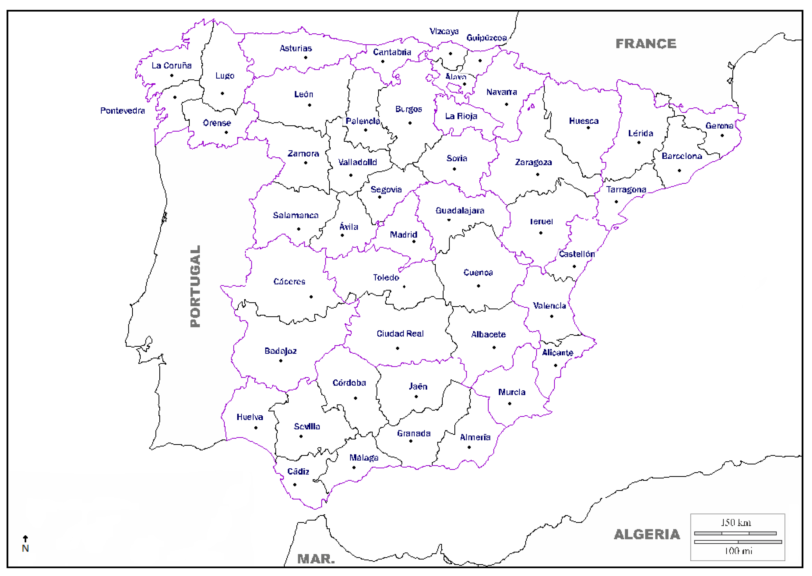
2.1. Study Area and General Climate Characteristics

Figure 1 presents the situation of each of the stations considered, one in each provincial capital (black points). In total, 47 temperature series and 47 precipitation series were analyzed, although the number of data in each ranges between 300 and 888.

Table 1. Information of the stations of the AEMET in provincial capitals, sample size, and period of data availability in this study for both variables.

Autonomy Community	Station	Period	Data Sample (n/num. years)	Altitude (m)	Latitude	Longitude
Aragón	Zaragoza	1983–2013	372/30	225	41°43′30″ N	00°48′39″ W
	Huesca	1983–2013	372/30	390	42°01′50″ N	00°35′05″ W
	Teruel	1983–2013	372/30	1043	40°32′30″ N	01°01′53″ W
Asturias	Oviedo	1972–2013	504/41	336	43°21′12″ N	05°52′27″ W
Cantabria	Santander	1954–2013	720/59	5	43°25′45″ N	03°49′53″ W
La Rioja	Logroño	1983–2013	372/30	353	42°27′08″ N	02°19′52″ W
Navarra	Pamplona	1954–2013	720/59	450	42°49′04″ N	01°38′18″ W
Basque Country	Vizcaya	1983–2013	372/30	29	43°17′26″ N	02°52′24″ W
	Gipuzkoa	1983–2013	372/30	251	43°18′23″ N	02°02′28″ W
	Álava	1983–2013	372/30	563	42°53′20″ N	02°40′22″ W
Galicia	A Coruña	1961–2013	636/52	58	43°21′57″ N	08°25′17″ W
	Pontevedra	1963–2013	600/50	108	42°26′18″ N	08°36′57″ W
	Ourense	1949–2013	780/64	400	42°25′10″ N	08°05′12″ W
	Lugo	1985–2013	348/28	445	43°06′41″ N	07°27′27″ W
Castile and León	Valladolid	1951–2013	756/62	735	41°38′27″ N	04°45′16″ W
	Ávila	1983–2013	372/30	1130	40°39′33″ N	04°40′48″ W
	Salamanca	1983–2013	372/30	775	40°57′27″ N	05°39′44″ W
	Palencia	1984–2013	360/29	874	41°59′44″ N	04°36′10″ W
	Segovia	1989–2013	300/24	1005	40°56′43″ N	04°07′35″ W
	Zamora	1983–2013	372/30	802	41°13′55″ N	05°29′52″ W
	Burgos	1983–2013	372/30	1001	42°19′20″ N	03°27′32″ W
	Soria	1983–2013	372/30	1082	41°46′30″ N	02°28′59″ W
	León	1983–2013	372/30	916	42°35′18″ N	05°39′04″ W
Castilla–La Mancha	Albacete	1967–2013	564/46	702	38°57′06″ N	01°51′45″ W
	Ciudad real	1971–2013	516/42	628	38°59′21″ N	03°55′13″ W
	Guadalajara	1949–2013	780/64	639	40°39′33″ N	03°10′24″ W
	Toledo	1975–2013	468/38	478	39°56′35″ N	03°54′57″ W
	Cuenca	1983–2013	372/30	900	40°04′30″ N	02°12′17″ W
Extremadura	Badajoz	1983–2013	372/30	185	38°53′00″ N	06°48′50″ W
	Cáceres	1983–2013	372/30	362	39°47′20″ N	06°23′37″ W
Madrid	Madrid	1983–2013	372/30	609	40°28′00″ N	03°33′20″ W
Cataluña	Tarragona	1984–2013	360/29	53	41°06′42″ N	01°08′42″ E
	Girona	1974–2013	480/39	143	41°54′42″ N	02°45′48″ E
	Lleida	1972–2013	504/41	217	41°36′32″ N	00°41′43″ E
	Barcelona	1968–2013	552/45	4	41°17′34″ N	02°04′12″ E
País Valenciano	Valencia	1983–2013	372/30	69	39°29′07″ N	00°28′28″ W
	Alicante	1968–2013	552/45	43	38°16′58″ N	00°34′15″ W
	Castellón	1976–2013	456/37	43	39°57′26″ N	00°04′19″ W
Murcia	Murcia	1983–2013	372/30	57	37°59′28″ N	01°07′42″ W
Andalucía	Jaén	1989–2013	300/24	580	37°46′39″ N	03°48′32″ W
	Sevilla	1962–2013	624/51	34	37°25′00″ N	05°52′45″ W
	Granada	1940–2013	888/73	690	37°08′10″ N	03°38′00″ W
	Málaga	1951–2013	756/62	500	36°46′42″ N	04°23′03″ W
	Almería	1968–2013	552/45	21	36°50′47″ N	02°21′25″ W
	Córdoba	1986–2013	336/27	90	37°50′39″ N	04°50′46″ W
	Cádiz	1983–2013	372/30	2	36°29′59″ N	06°15′28″ W
	Huelva	1983–2013	372/30	51	37°16′29″ N	06°50′17″ W

shows the information of the stations of the AEMET in peninsular province capitals. The first column shows the autonomous community to which each station belongs; the second column is the name of the city where the data collection station is located; the third column is the identified period of years for which data are available for both variables; the fourth column shows the number of data items for each series (n) together with the number of years comprising the period (number of years); the last three columns correspond to the geographic information (altitude, latitude, and longitude) that was used to obtain maps (Figure 1).

The climate of peninsular Spain is mainly divided into 3 types: oceanic, continental, and Mediterranean. Atlantic Spain (with an oceanic climate) extends from Galicia to the Pyrenees (Table 1—Galicia, Asturias, Cantabria, La Rioja, Navarra, and País Vasco). The Mediterranean inland climate extends mainly through the Central Plateau (Table 1—Castile and León, Castilla–La Mancha, and Extremadura). Its climate is Mediterranean but with continental characteristics due to the peninsular orography. The Mediterranean Coastal climate extends over the whole Mediterranean coast of Spain (Table 1—Cataluña, Comunidad Valenciana, and Murcia). The Andalusia region has all three characteristics: the Atlantic influence in its Atlantic coastal provinces (Huelva and Cádiz, oceanic climate), the Mediterranean with continental characteristics (Sevilla, Córdoba, and Jaén), and the Mediterranean (Granada, Málaga, and Almería) [34]. For the purposes of this study, 4 zones were considered taking into account the mentioned climate characteristics.

The first area is the north of peninsular Spain (zone I: Zaragoza, Huesca, Teruel, Oviedo, Santander, Logroño, Pamplona, Vizcaya, Gipuzkoa, Álava, A Coruña, Pontevedra, Ourense and Lugo);the second zone is the north and south plateau and the central system (zone II: Valladolid, Ávila, Salamanca, Palencia, Segovia, Zamora, Burgos, Soria, León, Albacete, Ciudad real, Guadalajara, Toledo, Cuenca, Badajoz, Cáceres, and Madrid);the third zone is the Mediterranean strip (zone III: Tarragona, Girona, Lleida, Barcelona, Valencia, Alicante, Castellón, and Murcia); and the fourth is the temperate Mediterranean zone (zone IV: Jaén, Sevilla, Granada, Málaga, Almería, Córdoba, Cádiz, and Huelva).

2.2. Statistical Analyses

Climate data analysis requires a study of homogeneity [35,36]. The climatic time series are influenced by inhomogeneities, i.e., non-climatic factors, such as changes in observational instruments, station relocations, and changes in station environment. A homogenous time series is defined as one where variations are caused only by variations in climate. Time series influenced by inhomogeneities may lead to deceptive conclusions regarding the state of climate and possible trends included [21]. In this study, we applied the tests of SNHT [37] to detect inhomogeneities in time series of temperature and precipitation. This was performed using Excel Statistics. The normality of climatic series was studied using the test of Lilliefors [38].

In order to detect the trend, an analytical adjustment by regression was made. In the description stage of the series, with the graphs of temperatures and precipitations time series, linear regression models were adjusted as a function of time, confirming the significance (+ or −) of coefficient b representing the slope of the straight line [39], and we completed the study using a Mann–Kendall trend test [40,41]. The magnitude of the trend with 95% confidence intervals was calculated using Sen’s slope [42].

The application of the Box–Jenkins methodology [43] requires values measured at regular intervals of time; therefore, we proceeded to complete missing data in each series considering that there was a low percentage (less than 1%) of missing data in the series analyzed. To complete each series, simple interpolation methods were used, as they are usually isolated values. In this case, the missing value in time t was completed with the mean of contiguous data (at times t − 1 and t + 1), or in case of any missing contiguous data, the average of the month was used [44]. This method was chosen after reviewing, checking, and comparing other methods in some stations and proving that the values obtained were not notably different from those obtained with the simple average method or regression methods [44]. Then, an exploratory analysis of data series was performed (outlier’s detection and lack of stationarity in means and variances).

The analysis of the series was carried out using ARIMA models based on stochastic process theory; obtaining the model assumes the existence of linear dependence between the variables whose values constitute the observed series [45]. The methodology used in this study for obtaining these models was established by [43]. With the complete and homogeneous series, the evolution graphs of the data as a function of time allow one to observe trends and possible periodicities, such as seasonality or variations in the dispersion. In relation to the analysis of trends, the word “trend” refers to a highly significant linear change (i.e., a level of confidence greater than 95%) in the value of some variable [46].

Given that these methods do not model well the trend in the case of lack of independence between the data, as occurs in the data of climatic series, the models based on stochastic processes, such as the ARIMA, adequately collect these dependencies due to the trend and seasonality. Thus, these variations were verified with the graphs of the simple autocorrelation function (ACF). In the case of trend, it was eliminated by taking differences of the type x_t − x_t−1 and, in case of seasonality, it was eliminated by taking differences of the type x_t − x_t−12 to obtain a stationary series. From the simple and partial autocorrelation functions (PAF) of the stationary series, it is possible to identify possible models that can represent the evolution of the observed data.

Given that the studied variables present seasonality, as they are monthly series of temperature and precipitation, the models to be estimated are of the SARIMA type (seasonal autoregressive integrated moving average), whose general representation is [43]:

ARIMA (p,d,q) × (P, D, Q)_s

where p is the number of AR parameters; q the number of MA parameters of the regular or non-seasonal part of the series; d is the number of non-seasonal differences, usually of the type x_t − x_t−1; P is the number of AR parameters of the seasonal part (SAR); Q is the number of MA parameters of the seasonal part (SMA);p and D is the number of differences with seasonal period s (in this case s = 12), usually x_t − x_t−12.

The estimation of the parameters of the model was made by optimization algorithms. Once the model was adjusted, the significance of the estimated coefficients was checked, and compliance with the hypotheses for these models was verified through the analysis of residues (randomness of the Box–Pierce test [47] and heteroscedasticity by test F for constant variance, comparing the 1st and 2nd half of the series). If the residues comply with the model hypothesis (p > 0.001), 12-month predictions are made that are compared with observed values of the 12 months of the year following the last of the series used to obtain the model. The average of those 12 errors will be close to zero.

The statistical software used was Excel Statistics, STATGRAPHICS Centurion XVII.I., Software R.

3. Results

3.1. Homogeneity Tests

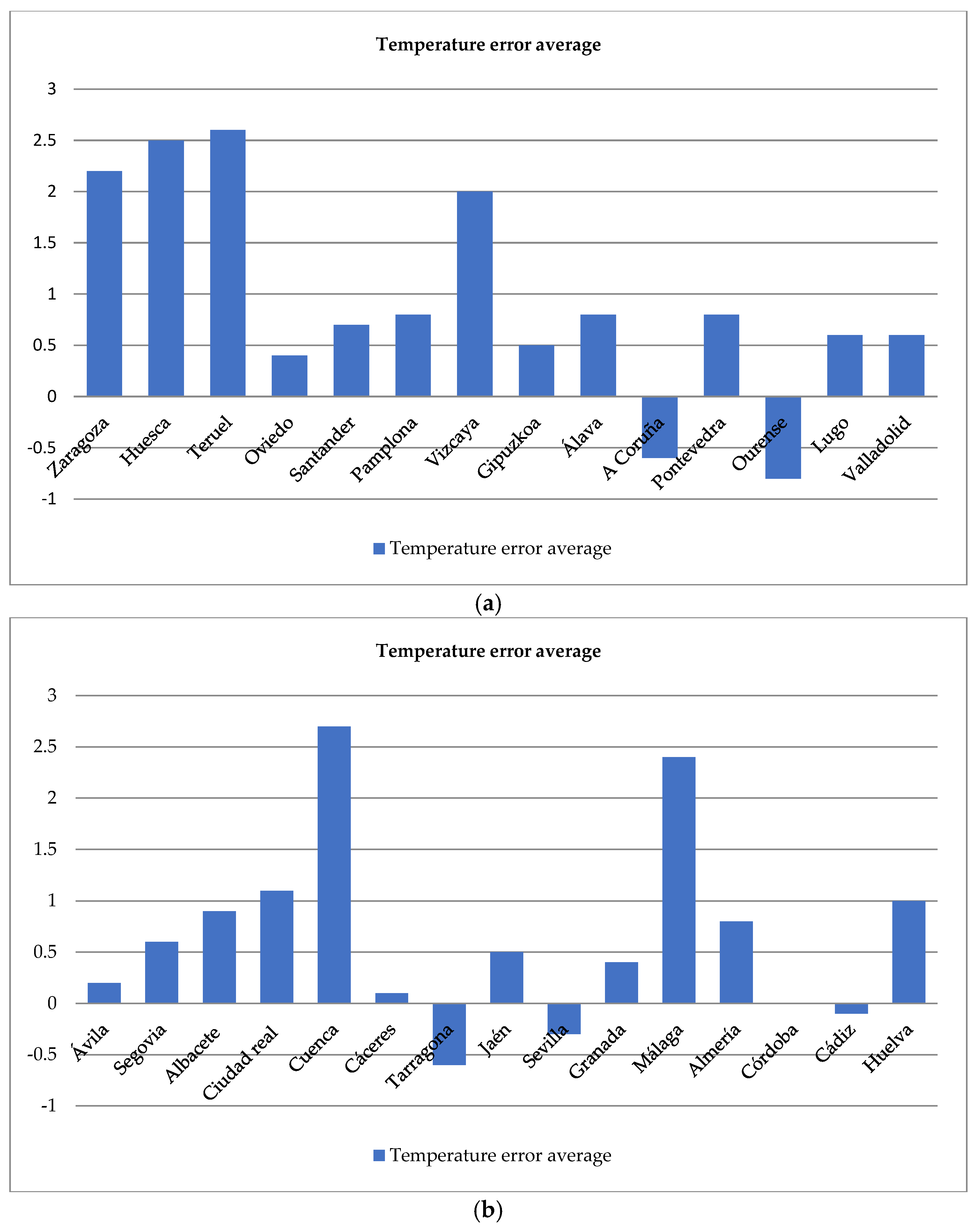
The SNHT homogeneity test allowed us to consider homogeneous data series (p > 0.01) except in Cantabria (p > 0.007), A Coruña (p > 0.001) Ourense, and Malaga (p < 0.0001). The time series for both temperature and precipitation did not give a normal distribution.

3.2. Trend Analysis

To obtain an ARIMA model, in the first stage, the graph of the data is observed as a function of time with the option of making a linear adjustment of the trend. The results of this option showed that in temperatures it is significant (p ≤ 0,05) in the series of Oviedo, Santander, A Coruña, Ourense, Valladolid, Salamanca, Albacete, Ciudad Real, Toledo, Girona, Barcelona, Castellón, Sevilla, Málaga, and Almería, with the magnitude varying between 0.0022 and 0.0074. That is, there were 15 series of temperatures with a significant, positive trend out of a total of 47. In precipitations, the trend was significant (p ≤ 0.05) for the case of Santander, Ourense, and Zamora (negative) with magnitudes of −0.041, −0.047 and −0.042, respectively, and Burgos and Jaén (positive) with magnitudes of 0.042 and 0.064, respectively (See

Table 2. Summary of results of the trend analysis for the temperature and precipitation series.

Province	Temperature Trend	Temperature Coefficient	Temperature p-Value	Precipitation Trend	Precipitation Coefficient	Precipitation p-Value
Oviedo	T = 11.6 + 0.0027t	0.0027	0.0246	N.S. (−)	−0.0005	0.972
Santander	T = 13.0 + 0.0025t	0.0025	0.0002	T = 122 − 0.041t	−0.041	0.00233
A Coruña	T = 13.2 + 0.0028t	0.0028	0.000064	N.S. (+)	0.0061	0.6424
Ourense	T = 6.5 + 0.0035t	0.0035	0.000007	T = 184 − 0.0476t	−0.0476	0.00305
Valladolid	T = 11.3 + 0.0022t	0.0022	0.0363	N.S. (+)	0.0035	0.495
Salamanca	T = 8.8 + 0.0063t	0.0063	0.0398	N.S. (−)	−0.0012	0.9265
Zamora	N.S. (+)	0.0006	0.8317	T = 54.8 − 0.042t	−0.042	0.002665
Burgos	N.S. (+)	0.001	0.7004	T = 27 + 0.0428t	0.0428	0.024354
Albacete	T = 11.7 + 0.0043t	0.0043	0.0175	N.S. (−)	−0.0033	0.6529
Ciudad real	T = 11.8 + 0.0063t	0.0063	0.0027	N.S. (+)	0.0082	0.4132
Toledo	T = 11.5 + 0.0074t	0.0074	0.0052	N.S. (−)	−0.0074	0.4645
Girona	T = 12 + 0.0047t	0.0047	0.01554	N.S. (−)	−0.0227	0.1918
Barcelona	T = 13.7 + 0.0042t	0.0042	0.003056	N.S. (−)	−0.0248	0.062
Castellón	T = 14.5 + 0.0051t	0.0051	0.007174	N.S. (+)	0.0042	0.7949
Jaén	N.S. (+)	0.0016	0.7098	T = 0.8 + 0.0647t	0.0647	0.0369
Sevilla	T = 17 + 0.004t	0.004	0.0028	N.S. (−)	−0.0227	0.0802
Málaga	T = 15 + 0.004t	0.004	0.000004	N.S. (−)	−0.0166	0.0802
Almería	T = 17.5 + 0.0026t	0.0026	0.0487	N.S. (−)	−0.0019	0.7477

N.S.: not significant.

). This trend must be considered orientative and deterministic. Therefore, with the non-parametric methods of Mann–Kendall and Sen’s slope (See

Table 3. Summary of results of the Mann–Kendall trend test and Sen’s Slope.

Province	Mann–Kendall Trend Test Temp.	Sen’s Slope Temp.	Mann–Kendall Trend Test Preci.	Sen’s Slope Preci.
Oviedo	a.h.: true	0.0026
Santander	a.h.: true	0.0023	a.h.: true	−0.03
A Coruña	a.h.: true	0.0028
Ourense	a.h.: true	0.0034	a.h.: true	−0.03
Valladolid	a.h.: true	0.0055
Salamanca	a.h.: true	0.0055
Zamora			a.h.: true	−0.022
Burgos			a.h.: true	0.04
Albacete	a.h.: true	0.0041
Ciudad real	a.h.: true	0.0061
Toledo	a.h.: true	0.0075
Girona	a.h.: true	0.0043
Barcelona	a.h.: true	0.0041
Castellón	a.h.: true	0.0049
Jaén			a.h.: true	0.03
Sevilla	a.h.: true	0.0039
Málaga	a.h.: true	0.004
Almería	a.h.: true	0.0024

a.h.: alternative hypothesis.

), it was compared with that obtained with the linear trend, and the results of positive trends in temperatures in the same weather stations coincide. Similarly, the positive precipitation trends in Burgos and Jaén and the negative precipitation trend in Santander, Ourense, and Zamora coincide.

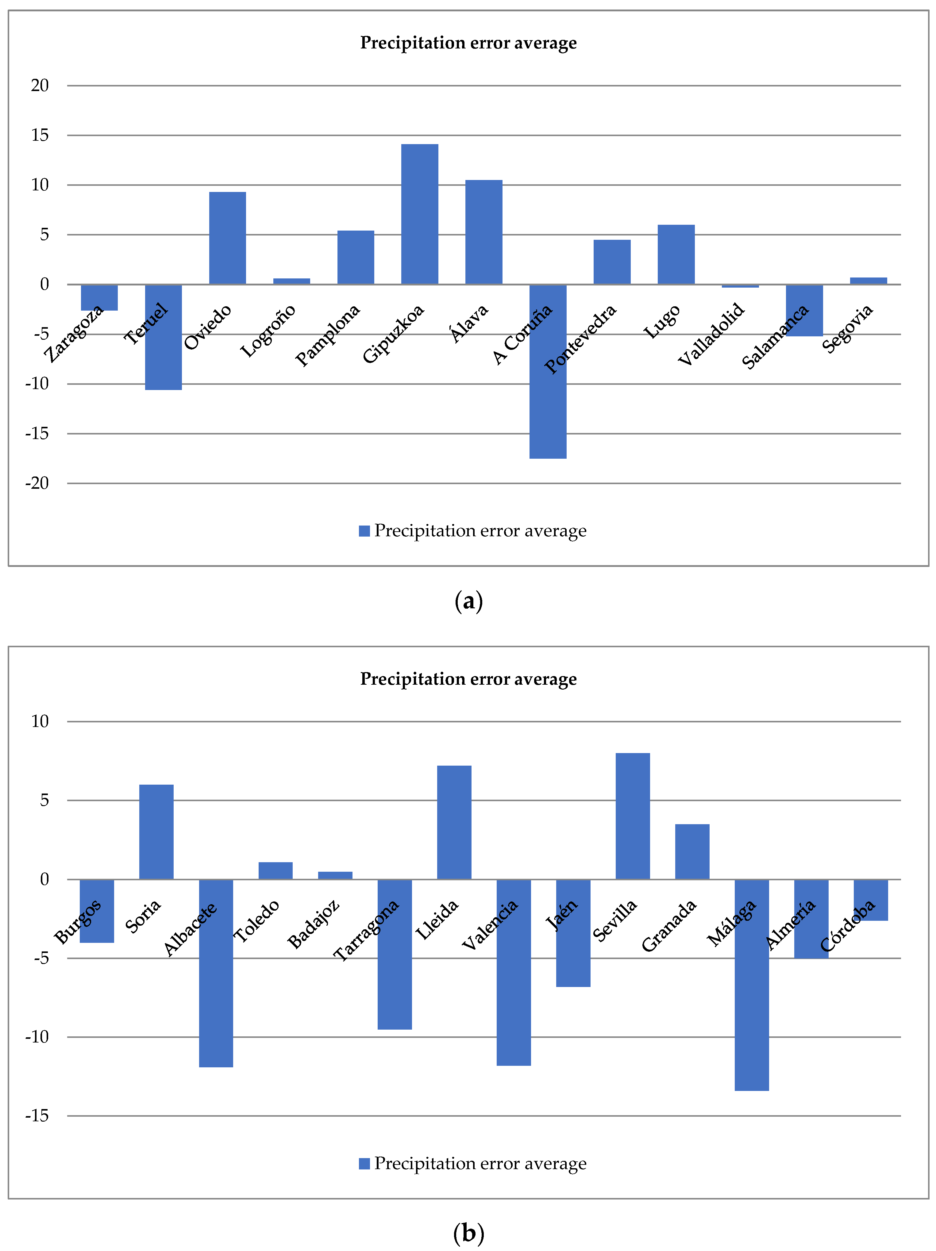
3.3. ARIMA Modeling and Forecasting

The 29 differentiated temperature series allowed for the identification of ARIMA models. A summary of the resulting models obtained for each of the 29 temperature series is shown in the

Table 4. ARIMA models of the 29 temperature series of peninsular Spain.

Serie	Model	Estimated Coefficients (p ≤ 0.05)
Zaragoza	ARIMA (1,1,1) × (0,1,1)12	Wt = 0.133Wt−1 + 0.922at−1 + 0.912at−12 + at 0.019  0.000  0.000  $\leftarrow$p-v
Huesca	ARIMA (1,1,1) × (0,1,1)12	Wt = −0.001 + 0.242Wt−1 + 0.942at−1 + 0.905at−12 + at 0.000  0.000  0.000  $\leftarrow$p-v
Teruel	ARIMA (1,0,0) × (0,1,1)12	Zt = 0.302Zt−1 + 0.948at−12 + at 0.000  0.000  $\leftarrow$p-v
Oviedo	ARIMA (1,0,0) × (0,1,1)12	Zt = 0.024 + 0.17Zt−1 + 0.948at−12 + at 0.000  0.000  $\leftarrow$p-v
Santander	ARIMA (1,0,0) × (0,1,1)12	Zt = 0.022 + 0.221Zt−1 + 0.964at−12 + at 0.000  0.000  $\leftarrow$p-v
Pamplona	ARIMA (1,0,0) × (0,1,1)12	Zt = 0.013 + 0.19Zt−1 + 0.96at−12 + at 0.000  0.000  $\leftarrow$p-v
Vizcaya	ARIMA (1,0,1) × (0,1,1)12	Zt = 0.632Zt−1 + 0.466at−1 + 0.939at−12 + at 0.002  0.044  0.000  $\leftarrow$p-v
Gipuzkoa	ARIMA (1,0,0) × (0,1,1)12	Zt = 0.139Zt−1 + 0.938at−12 + at 0.008  0.000  $\leftarrow$p-v
Álava	ARIMA (1,0,1) × (0,1,1)12	Zt = 0.011 + 0.686Zt−1 + 0.535at−1 + 0.935at−12 + at 0.000  0.012  0.000  $\leftarrow$p-v
A Coruña	ARIMA (1,0,1) × (0,1,1)12	Zt = 0.013 + 0.557Zt−1 + 0.349at−1 + 0.96at−12 + at 0.000  0.038  0.000  $\leftarrow$p-v
Pontevedra	ARIMA (1,0,0) × (0,1,1)12	Zt = −0.007 + 0.218Zt−1 + 0.936at−12 + at 0.000  0.000  $\leftarrow$p-v
Ourense	ARIMA (1,1,1) × (0,1,1)12	Wt = 0.205Wt−1 + 0.949at−1 +0.959at−12 + at 0.000  0.000  0.000  $\leftarrow$p-v
Lugo	ARIMA (1,0,0) × (0,1,1)12	Zt = 0.019 + 0.161Zt−1 + 0.936at−12 + at 0.03  0.00  $\leftarrow$p-v
Valladolid	ARIMA (1,0,0) × (0,1,1)12	Zt = 0.019 + 0.206Zt−1 + 0.963at−12 + at 0.000  0.000  $\leftarrow$p-v
Ávila	ARIMA (1,0,0) × (0,1,1)12	Zt = −0.05 + 0.177Zt−1 +0.937at−12 + at 0.000  0.000  $\leftarrow$p-v
Segovia	ARIMA (1,0,0) × (0,1,1)12	Zt = 0.209Zt−1 + 0.927at−12 + at 0.000  0.000  $\leftarrow$p-v
Albacete	ARIMA (1,1,1) × (0,1,1)12	Wt = 0.156Wt−1 + 0.97at−1 + 0.943at−12 + at 0.000  0.000  0.000  $\leftarrow$p-v
Ciudad real	ARIMA (1,1,1) × (0,1,1)12	Wt = −0.0004 + 0.25Wt−1 + 0.985at−1 + 0.918at−12 + at 0.000  0.000  0.000  $\leftarrow$p-v
Cuenca	ARIMA (1,0,0) × (0,1,1)12	Zt = 0.233Zt−1 + 0.923at−12 + at 0.000  0.000  $\leftarrow$p-v
Cáceres	ARIMA (1,0,0) × (1,1,1)12	Zt = 0.025 + 0.237Zt−1 + 0.047zt−12 + 0.941at−12 + at 0.393  0.000  $\leftarrow$p-v
Tarragona	ARIMA (1,0,0) × (0,1,1)12	Zt = −0.03 + 0.324Zt−1 + 0.8986at−12 + at 0.000  0.000  $\leftarrow$p-v
Jaén	ARIMA (1,0,0) × (0,1,1)12	Zt = 0.233Zt−1 + 0.935at−12 + at 0.000  0.000  $\leftarrow$p-v
Sevilla	ARIMA (1,0,0) × (0,1,1)12	Zt = 0.031 + 0.258Zt−1 + 0.921at−12 + at 0.000  0.000  $\leftarrow$p-v
Granada	ARIMA (1,1,1) × (0,1,1)12	Wt = 0.215Wt−1 + 0.977at−1 + 0.968at−12 + at 0.000  0.000  $\leftarrow$p-v
Málaga	ARIMA (1,1,1) × (0,1,1)12	Wt = 0.266Wt−1 + 0.915at−1 + 0.969at−12 + at 0.000  0.000  $\leftarrow$p-v
Almería	ARIMA (1,1,1) × (0,1,1)12	Wt = 0.229Wt−1 + 0.975at−1 + 0.938at−12 + at 0.000  0.000  0.000  $\leftarrow$p-v
Córdoba	ARIMA (0,0,1) × (0,1,1)12	Zt = 0.029−0.277at−1 + 0.933at−12 + at 0.000  0.000  $\leftarrow$p-v
Cádiz	ARIMA (0,0,1) × (0,1,1)12	Zt = 0.02−0.28at−1 + 0.942at−12 + at 0.000  0.000  $\leftarrow$p-v
Huelva	ARIMA (1,0,1) × (0,1,1)12	Zt = −0.008 + 0.7Zt−1 + 0.447at−1 + 0.942at−12 + at 0.000  0.001  0.000  $\leftarrow$p-v

p-v: p-value.

.

The ARIMA model of prediction without the constant that allowed for the estimation of the values of the variable at a future time (t + 1) based on their values at previous instants (t, t − 1, ...) for the temperature series of Zaragoza, Huesca, Ourense, Albacete, Ciudad Real, Granada, Málaga, and Almería resulted in the following:

$$\begin{array}{c}\mathrm{ARIMA} (1,1,1)\times (0,1,1{)}_{12}: W_t=\varnothing W_{t-1}-\mathsf{\theta }{a}_{t-1}-\vartheta a_{t-12}+a_t;W_t=Z_t-Z_{t-1}; Z_t=X_t-X_{t-12}\\ Z_t=Z_{t-1}+\varnothing \left(Z_{t-1}-Z_{t-2}\right)-\mathsf{\theta }{a}_{t-1}-\vartheta a_{t-12}+a_t\\ X_t=X_{t-12}+\left(1+\varnothing )(X_{t-1}-X_{t-13}\right)-\varnothing \left(X_{t-2}-X_{t-14}\right)-\mathsf{\theta }{a}_{t-1}-\vartheta a_{t-12}+a_t\end{array}$$

(1)

For the temperature series of Teruel, Oviedo, Santander, Pamplona, Gipuzkoa, Pontevedra, Lugo, Valladolid, Ávila, Segovia, Cuenca, Tarragona, Jaén, and Sevilla, the prediction model without the constant was

$$\begin{array}{c}\mathrm{ARIMA} (1,0,0)\times (0,1,1{)}_{12}: Z_t=\varnothing Z_{t-1}+\vartheta a_{t-12}+a_t; Z_t=X_t-X_{t-12}\\ X_t=X_{t-12}+\varnothing (X_{t-1}-X_{t-13})-\vartheta a_{t-12}+a_t\end{array}$$

(2)

For the temperature series of Vizcaya, Álava, A Coruña, and Huelva, the prediction model without the constant was:

$$\begin{array}{c}\mathrm{ARIMA} (1,0,1)\times (0,1,1{)}_{12}: Z_t=\varnothing Z_{t-1}-\mathsf{\theta }{a}_{t-1}-\vartheta a_{t-12}+a_t\\ X_t=X_{t-12}+\varnothing \left(X_{t-1}-X_{t-13}\right)-\mathsf{\theta }{a}_t-\vartheta a_{t-12}+a_t\end{array}$$

(3)

For the Cáceres temperature series, the prediction model without the constant was

$$\mathrm{ARIMA} (1,0,0)\times (1,1,1{)}_{12}: X_t=X_{t-12}+\varnothing (X_{t-1}-X_{t-13})+\alpha (X_{t-12}-X_{t-24})-\vartheta a_{t-12}+a_t$$

(4)

For the temperature series of Córdoba and Cádiz, the prediction model without the constant was

$$\mathrm{ARIMA} (0,0,1)\times (0,1,1{)}_{12}: X_t=X_{t-12}-\mathsf{\theta }{a}_{t-1}-\vartheta a_{t-12}+a_t$$

(5)

where in Equations (1)–(5), $\varnothing ,\mathsf{\theta },\vartheta , and \alpha$ represent the estimated coefficient for each model.

A summary of the resulting models obtained for each of the 27 precipitation series is shown in the

Table 5. ARIMA models of the 27 precipitation series.

Serie	Model	Estimated Coefficients (p ≤ 0.05)
Zaragoza	ARIMA (0,0,0) × (0,1,1)12	Zt = 0.951at−12 + at 0.000  $\leftarrow$p-v
Teruel	ARIMA (1,1,1) × (0,1,1)12	Wt = 0.108Wt−1 + 0.976at−1 +0.936at−12 + at 0.042 0.000  0.000  $\leftarrow$p-v
Oviedo	ARIMA (1,0,0) × (0,1,1) 12	Zt = 0.015 + 0.113Zt−1 + 0.948at−12 + at 0.011 0.000  $\leftarrow$p-v
Logroño	ARIMA (1,0,0) × (0,1,1)12	Zt = 0.127Zt−1 + 0.909at−12 + at 0.0015 0.000  $\leftarrow$p-v
Pamplona	ARIMA (1,0,0) × (0,1,1)12	Zt = 0.116Zt−1 + 0.957at−12 + at 0.001 0.000  $\leftarrow$p-v
Gipuzkoa	ARIMA (0,0,0) × (0,1,1)12	Zt = 0.928at−12 + at 0.000  $\leftarrow$p-v
Álava	ARIMA (0,0,0) × (0,1,1)12	Zt = 0.925at−12 + at 0.000  $\leftarrow$p-v
A Coruña	ARIMA (1,0,0) × (0,1,1)12	Zt = 0.116Zt−1 + 0.957at−12 + at 0.003 0.000  $\leftarrow$p-v
Pontevedra	ARIMA (1,0,0) × (0,1,1)12	Zt = 0.1Zt−1 + 0.958at−12 + at 0.015 0.000  $\leftarrow$p-v
Lugo	ARIMA (1,0,0) × (0,1,1)12	Zt = 0.272Zt−1 + 0.94at−12 + at 0.000  0.000  $\leftarrow$p-v
Valladolid	ARIMA (0,0,0) × (0,1,1)12	Zt = 0.962at−12 + at 0.000  $\leftarrow$p-v
Salamanca	ARIMA (0,0,0) × (0,1,1)12	Zt = 0.94at−12 + at 0.000  $\leftarrow$p-v
Segovia	ARIMA (1,0,0) × (0,1,1)12	Zt = 0.124Zt−1 + 0.925at−12 + at 0.035 0.000  $\leftarrow$p-v
Burgos	ARIMA (0,0,0) × (0,1,1)12	Zt = 0.935at−12 + at 0.000  $\leftarrow$p-v
Soria	ARIMA (1,0,0) × (0,1,1)12	Zt = 0.167Zt−1 + 0.939at−12 + at 0.001 0.000  $\leftarrow$p-v
Albacete	ARIMA (0,1,1) × (0,1,1)12	Zt = 0.968at−1 + 0.945at−12 + at 0.000  0.000  $\leftarrow$p-v
Toledo	ARIMA (0,0,1) × (0,1,1)12	Zt = −0.176at−1 + 0.947at−12 + at 0.000  0.000  $\leftarrow$p-v
Badajoz	ARIMA (1,0,0) × (0,1,1)12	Zt = 0.178Zt−1 + 0.934at−12 + at 0.000  0.000  $\leftarrow$p-v
Tarragona	ARIMA (0,0,0) × (0,1,1)12	Zt = −0.354 + 0.935at−12 + at 0.000  $\leftarrow$p-v
Lleida	ARIMA (0,0,0) × (0,1,1)12	Zt = 0.953at−12 + at 0.000  $\leftarrow$p-v
Valencia	ARIMA (0,0,0) × (0,1,1) 12	Zt = 0.944at−12 + at 0.000  $\leftarrow$p-v
Jaén	ARIMA (1,0,0) × (0,1,1)12	Zt = 0.205Zt−1 + 0.921at−12 + at 0.000  0.000  $\leftarrow$p-v
Sevilla	ARIMA (1,0,0) × (0,1,1)12	Zt = 0.134Zt−1 + 0.964at−12 + at 0.000  0.000  $\leftarrow$p-v
Granada	ARIMA (1,0,0) × (0,1,1)12	Zt = 0.121Zt−1 + 0.968at−12 + at 0.000  0.000  $\leftarrow$p-v
Málaga	ARIMA (0,0,1) × (0,1,1)12	Zt = −0.117at−1 + 0.971at−12 + at 0.001 0.000  $\leftarrow$p-v
Almería	SARIMA (0,1,1)12	Zt = 0.97at−12 + at 0.000  $\leftarrow$p-v
Córdoba	ARIMA (1,0,0) × (1,1,1)12	Zt = 0.21 + 0.16Zt−1 + 0.12Zt−12 + 0.94at−12 + at 0.004 0.04 0.000  $\leftarrow$p-v

p-v: p-value.

.

The ARIMA model of prediction without the constant that allowed for the estimation of the values of the variable at a future time (t + 1) based on their values at previous instants (t, t–1, …) for the precipitation series of Zaragoza, Gipuzkoa, Álava, Valladolid, Salamanca, Burgos, Tarragona, Lleida, Valencia, and Almería resulted in the following:

$$\begin{array}{c}\mathrm{SARIMA} (0,1,1{)}_{12}: Z_t=\vartheta a_{t-12}+a_t; Z_t={-}_t-X_{t-12}\\ X_t=X_{t-12}+\vartheta a_{t-12}+a_t\end{array}$$

(6)

For the Teruel precipitation series, the prediction model without the constant was

$$\begin{array}{c}\mathrm{ARIMA} (1,1,1)\times (0,1,1{)}_{12}: W_t=\varnothing W_{t-1}-\mathsf{\theta }{a}_{t-1}-\vartheta a_{t-12}+a_t; W_t=Z_t-Z_{t-1}; Z_t=X_t-X_{t-12}\\ Z_t=Z_{t-1}+\varnothing \left(Z_{t-1}-Z_{t-2}\right)-\mathsf{\theta }{a}_{t-1}-\vartheta a_{t-12}+a_t\\ X_t=X_{t-12}+\left(1+\varnothing )(X_{t-1}-X_{t-13}\right)-\varnothing \left(X_{t-2}-X_{t-14}\right)-\mathsf{\theta }{a}_{t-1}-\vartheta a_{t-12}+a_t\end{array}$$

(7)

For the precipitation series of Oviedo, Logroño, Pamplona, A Coruña, Pontevedra, Lugo, Segovia, Soria, Badajoz, Jaén, Sevilla, and Granada, the prediction model without the constant was

$$\begin{gathered} \mathrm{ARIMA} (1,0,0)\times (0,1,1{)}_{12}: Z_t=\varnothing Z_{t-1}+\vartheta a_{t-12}+a_t; Z_t={-}_t-X_{t-12} \\ {X}_t=X_{t-12}+\varnothing (X_{t-1}-X_{t-13})-\vartheta a_{t-12}+a_t \end{gathered}$$

(8)

For the precipitation series of Albacete, the prediction model without the constant was

$$\begin{gathered} \mathrm{ARIMA} (0,1,1)\times (0,1,1{)}_{12}: Z_t=\mathsf{\theta }{a}_{t-1}+\vartheta a_{t-12}+a_t; Z_t={-}_t-X_{t-12} \\ {X}_t=X_{t-12}+\mathsf{\theta }{a}_{t-1}+\vartheta a_{t-12}+a_t \end{gathered}$$

(9)

For the precipitation series of Toledo and Málaga, the prediction model without the constant was

$$\begin{gathered} \mathrm{ARIMA} (0,0,1)\times (0,1,1{)}_{12}: Z_t=\mathsf{\theta }{a}_{t-1}+\vartheta a_{t-12}+a_t; Z_t={-}_t-X_{t-12} \\ {X}_t=X_{t-12}+\mathsf{\theta }{a}_{t-1}+\vartheta a_{t-12}+a_t \end{gathered}$$

(10)

For the precipitation series of Córdoba, the prediction model without the constant was

$$X_t=X_{t-12}+\varnothing (X_{t-1}-X_{t-13})+\alpha (X_{t-12}-X_{t-24})-\vartheta a_{t-12}+a_t$$

(11)

where in Equations (6)–(11), $\varnothing ,\mathsf{\theta },\vartheta , and \alpha$ represent the estimated coefficient for each model.

4. Discussion

The homogeneity tests, according to [48], were considered valid for use in this study, because the removal of false detected inhomogeneities and the acceptance of inhomogeneous series affect each subsequent analysis (e.g., trend assessments and extreme analysis).

The study revealed the existence of a significant, positive trend in the temperature series of Oviedo, Santander, A Coruña, and Ourense with the magnitude from 0.002 to 0.003 belonging to study zone I. In the same zone, it was also observed that positive trends clearly prevailed over negative trends in the periods of the study. “The increase in global temperature is not homogeneously distributed on the surface, varying in magnitude between different regions and between different locations within the same region. These regional variations are also perceived in the behavior of extreme values and in the daily thermal amplitude, which exhibits negative trends in many regions of the globe, while in others the changes are of opposite sign or are not significant. The comparison between different papers is also complicated, since the periods of study, the variables analyzed, the stations of measurement selected and the time scale used (daily, monthly, seasonal or annual) do not coincide in most cases and the results show a high sensitivity to all these factors [46]”. However, several authors detected a positive trend of temperatures in Spain, and despite the differences between the periods analyzed and the time scales, they found results almost similar to ours. González-Hidalgo et al. [49] identified a positive and significant global signal in the period 1951–2010 in the analysis of trends of mean monthly maximum temperatures (Tmax) and mean monthly minimum temperatures (Tmin) in peninsular Spain with the MOTEDAS database. Cruz et al. [50] found for the mean monthly temperatures of Galicia in the period of 1973–2004, there was a significant increase in the mean temperature in the months of January, March, May, June, and August, leaving February, April, and July close to significance. Brunet et al. [51] found a significant, positive trend for the spatial pattern of the northern zone of Spain and that the annual averages of the mean daily temperature had increased significantly in the period of 1805–2005. Del Rio et al. [52] highlighted the significant, positive trends for the mean monthly temperatures from 1961 to 2006 and revealed that the temperature had generally increased during all months and seasons of the year during the last four decades, and they also detected for the same period a significant, positive trend of mean monthly temperatures in the Cantabrian cornice and in the Galician massif in the months of March and June. It should be noted that of the fourteen series of mean monthly temperatures of zone I, only four series showed a significant, positive trend. Those were the temperature series of Oviedo, Santander, A Coruña, and Ourense; the remaining series did not present a significant trend. This shows the existence of what is called the “Hiatus”, defined as the absence of a significant trend [49,53,54].

Our study revealed the existence of a significant, positive trend for the temperature series of Valladolid, Salamanca, Albacete, Ciudad Real, and Toledo with the magnitude from 0.004 to 0.007 in zone II, which is located in the Central Plateau. Positive trends in zone II clearly prevailed over negative trends in the periods of study as in the case of zone I. Several studies focused on the north and south plateau and the Spanish central system, examining the trends of the climatic variable temperature. Such studies found results almost similar to ours, despite the differences in the periods analyzed and the time scales. For example, Morales et al. [55] detected a positive trend at the 95% confidence level by analyzing the annual maximums and mean temperatures in winter for Castile and León in the period of 1945–1996. Del Río et al. [56] detected a positive trend of mean monthly maximum and minimum temperatures in every month of the year for Castile and León in the period 1961–1997. Labajo et al. [57] detected a positive trend of the mean annual minimum temperature for Castile and León in the period 1945–1994. Del Río et al. [58] found positive trends in the mean annual temperature for Castile and León in the period of 1961–1997.

The trends detected in zone III showed a significant, positive trend for the temperature series of Girona, Barcelona, and Castellón with a magnitude from 0.004 to 0.005 for the three series. Other authors also detected a positive trend of temperatures in the Mediterranean strip despite the differences in the periods analyzed and the time scales. For example, Brunet et al. [12] detected a significant, positive trend for the Mediterranean strip (Barcelona, Valencia, Alicante, and Murcia) for annual maximum and minimum temperatures in the period of 1850–2003. El Kenawy et al. [59] detected the predominance of a significant, positive trend of annual maximum and minimum temperatures in the period of 1950–2006 for the Mediterranean strip (Tarragona, Girona, Lleida, Barcelona, and Castellón). Oñate et al. [60] detected a significant, positive trend of mean annual temperatures for Alicante since 1901.

The study zone IV showed a significant, positive trend for the temperatures series of Sevilla, Málaga, and Almería with a magnitude from 0.002 to 0.004.

Regarding precipitation, the study revealed the existence of a significant, negative trend for series of Santander and Ourense with a magnitude of −0.04 in zone I and for series of Zamora with a magnitude of −0.04 in zone II and a significant, positive trend for series of Burgos and Jaén with magnitude of 0.04 and 0.06, respectively, in zones II and IV. Regarding precipitation in peninsular Spain, in the analysis of the monthly, annual, and seasonal series, no significant trends were observed throughout the 20th century as pointed out by several studies [23,36,61,62,63,64,65,66,67]. However, Mosmann et al. [68] detected a statistically significant, positive trend in large areas of continental Spain in the analysis of precipitation series in 333 summer precipitation stations in the period of 1961–1990.Therefore, “when studies on precipitation trends in the peninsular Spain are contrasted, it is common to find discrepancies and contradictions in the results, even when it comes to trends related to the same period. The disagreements are usually due to the existence of multiple regional databases of precipitation stations with very variable density, often unpublished or with very restricted access, there being little coincidence between the series analyzed by different studies. Other causes may be differences in the statistical methods used, problems with the quality and homogenization of the data and the lack of a unified methodology to correct these problems and another complication that arises is that, due to the great spatial variability of the precipitation, changes in local precipitation are not necessarily representative of changes on a larger scale” [46]. However, there are several studies on precipitation trends in peninsular Spain and some results, coincide with the trend detected in our study area (zone I) despite the differences in the periods analyzed and the time scales, while others found different results from ours. For example, González-Hidalgo et al. [28] detected a negative trend of monthly precipitation in the month of March for the Galician massif, while the Cantabrian cornice presented a non-significant trend in the period of 1946–2005. Serrano et al. [69] detected a positive trend of mean monthly precipitation in the cold months and in summer during the period of 1919–1992 in Galicia and the Cantabrian coast. Cuadrat et al. [70] detected a negative trend of monthly precipitation for Zaragoza, Huesca, and Teruel in the period of 1950–2010. Esteban-Parra et al. [23] found a positive trend of annual precipitation for the Cantabrian stations in the period of 1880–1992. Serrano et al. [61] detected a non-significant trend in the Cantabrian cornice and the Galician massif in the analysis of annual precipitation in the period of 1921–1995. De Luis et al. [71] detected a negative trend of annual and seasonal precipitation in the period of 1951–2000 in the Ebro basin, including the territories of the autonomous communities of the Basque Country, Cantabria, Castile and León, La Rioja, Navarra, Aragón, Cataluña, Castilla–La Mancha, and the Comunidad Valenciana.

In zone II of the study, negative trends prevailed over positive trends in the periods of study. Several studies detected negative trends in precipitation at the level of peninsular Spain [24,25,72,73] despite the differences in the periods analyzed and the time scales. At the level of the plateau, Del Río et al. [58] observed a statistically significant, negative trend in March in the precipitation for Castile and León during three seasons (winter, spring, and autumn) in the period of 1961–1997. González-Hidalgo et al. [27,28] detected a significant, negative trend with the total precipitation during the month of March for the north–south plateau and the central system of peninsular Spain in the analysis of monthly precipitation in the period of 1946–2005.

In zone III, negative trends prevailed over positive trends in the periods of study. De Luis et al. [74] observed that the negative trend predominated in the analysis of the annual precipitation in the Valencian Community during the period of 1961–1990. Álvarez et al. [75] detected a slight statistically insignificant, negative trend in the mean annual precipitation series of the Region of Murcia in the period of 1914–2013. Guirado and Bermúdez [76] showed a slight negative trend of annual precipitation in Murcia in the period of 1933–2008. González-Hidalgo et al. [77] detected for the month of March a significant, negative trend for monthly precipitation that affected the entire Mediterranean strip in the period of 1951–2000. Romero et al. [78] detected a negative trend of daily precipitation in western Catalonia in the period of 1964–1993. Lana et al. [79] detected a significant, negative trend of daily precipitation in Cataluña in the period of 1950–2000. De Luis et al. [80] detected a significant, negative trend of annual precipitation in the Valencian Community in the period of 1961–1990.Similarly to us, Moreno and Martín-Vide also detected a negative trend in precipitation in the Mediterranean strip, while Quereda et al., in an analysis of 11 long series, found an increase in Cataluña and Castellon [81].

In zone IV, no negative or positive trend clearly prevailed in the periods of study, and the authors González-Hidalgo JC et al. also mentioned that “no homogeneous or global behavior of monthly precipitation trends was observed” in the Mediterranean strip of peninsular Spain [77].

Several authors have conducted studies for predictions with ARIMA modelling [82,83]. Temperature and precipitation data recorded in 47stations from different climatic zones of peninsular Spain were used to create suitable ARIMA models. Of the 47 temperature series, only 29 complied with the contrasts of the randomness of Box–Pierce and heteroscedasticity for constant variance; comparing the first and second half of the series and the 47 precipitation series, only 27 complied with these contrasts.

In addition, of the 29 temperature series and 27 precipitation series, the coefficients of the autocorrelation functions for multiple lags of the seasonal period were significantly different from zero. Therefore, a seasonal order differencing was made. Thus, D = 1. In order to establish the best ARIMA models for temperature and precipitation series, we used parameters p and q between 0 and 1 for optimization. All the ARIMAs of the 29 temperature series and 27 precipitation series were selected with the lowest possible RMSE error (root mean squared error). The RMSE ranged from 0.931206 (corresponding to the Almería temperature series) to 1.64402 (corresponding to the Teruel temperature series). For the precipitation series, the RMSE varied from 21.99 (corresponding to the Almería series) to 98,978 (corresponding to the Pontevedra series). Lastly, the ARIMA models obtained in Table 4 and Table 5 could be beneficial in numerous applications where the observed temperature records are quite short or incomplete, or lack spatial coverage [84]. Moreover, the errors did not exceed 3 °C for the monthly average in temperatures and 20 mm in rainfall (see Figure 2a,b and Figure 3a,b); therefore, they can be useful for local short-term predictions (12 months) in practical situations, such as forest fires and pests and diseases in wild plants or cultivated and agricultural crops.

5. Conclusions

The Box–Jenkins methodology allowed us to model the variations in temperatures and precipitations produced over time in the 47 provinces of peninsular Spain by grouping provinces into four zones. In the trend analysis of the 47 temperature series, only 34.04% showed a significant, positive trend. Among the 47 temperatures series in peninsular Spain, it was possible to correctly adjust a model for 29 series (or 61.7%), while the remaining 18 series (or 38.3%) did not correctly adjust. In the trends analysis of the 47 precipitation series, only those of Santander, Ourense, and Zamora (or a total of 6.3%) presented a significant, negative trend, while the precipitation series of Burgos and Jaén (4.2%) presented a significant, positive trend. Among the 47 precipitations series in peninsular Spain, it was possible to correctly adjust a model for 27 series (or 57.4%), while the remaining 20 series (or 42.6%) did not correctly adjust to a model.

References

1. Vinnikov, K.Y.; Groisman, P.Y.; Lugina, K.M. Empirical Data on Contemporary Global Climate Changes (Temperature and Precipitation). J. Clim. 1990, 3, 662–677. [Google Scholar] [CrossRef] [Green Version]
2. Jones, P.D.; Raper, S.C.B.; Wigley, T.M.L. Southern Hemisphere Surface Air Temperature Variations: 1851–1984. J. Clim. Appl. Meteorol. Climatol. 1986, 25, 1213–1230. [Google Scholar] [CrossRef] [Green Version]
3. Hansen, J.; Lebedeff, S. Global Trends of Measured Surface Air Temperature. J. Geophys. Res. 1987, 92, 345–372. [Google Scholar] [CrossRef] [Green Version]
4. Visser, H.; Molenar, J. Trend Estimation and Regression Analysis in Climatological Time Series: An application of Structural Time Series Models and Kalman Filter. J. Clim. 1995, 8, 969–979. [Google Scholar] [CrossRef] [Green Version]
5. Zheng, X.; Basher, R.E. Structural Time Series Models and Trend Detection in Global and Regional Temperature Series. J. Clim. 1999, 12, 2347–2358. [Google Scholar] [CrossRef]
6. Seater, J.J. World Temperature-Trend Uncertainties and Their Implications for Economic Policy. J. Bus. Econ. Stat. 1993, 11, 265–277. [Google Scholar] [CrossRef]
7. Harvey, D.I.; Mills, T.C. Modelling Global Temperature Trends Using Cointegration and Smooth Transition. Stat. Model. 2001, 1, 143–159. [Google Scholar] [CrossRef]
8. Mudelsee, M. Trend Analysis of Climate Time Series: A Review of Methods. EarthSci. Rev. 2019, 190, 310–322. [Google Scholar] [CrossRef]
9. Schönwiese, C.D.; Rapp, J. Climate Trend Atlas of Europe Based on Observations 1891–1990; Kulver Academic Publishers: Dordrecht, The Netherlands, 1997; p. 235. [Google Scholar] [CrossRef]
10. Klein Tank, A.M.G.; Können, G.P.; Selten, F.M. Signals of Anthropogenic Influence on European Warming as Seen in the Trends Patterns of Daily Temperature Variance. Int. J. Climatol. 2005, 25, 1–16. [Google Scholar] [CrossRef]
11. Moberg, A.; Jones, P.D.; Lister, D.; Walther, A.; Brunet, M.; Jacobeit, J.; Alexander, L.V.; Della-Marta, P.M.; Luterbacher, J.; Yiou, P.; et al. Indices for Daily Temperature and Precipitation Extremes in Europe Analyzed for the Period 1901–2000. J. Geophys. Res. Atmos. 2006, 111, 1–25. [Google Scholar] [CrossRef] [Green Version]
12. Brunet, M.; Saladié, O.; Jones, P.D.; Sigró, J.; Aguilar, E.; Moberg, A.; Lister, D.; Walther, A.; López, D.; Almarza, C. The Development of a New Dataset of Spanish Daily Adjusted Temperature Series (SDATS) (1850–2003). Int. J. Climatol. 2006, 26, 1777–1802. [Google Scholar] [CrossRef]
13. Prieto, L.; García Herrera, R.; Díaz, J.; Hernández, E.; del Teso, T. Minimum Extreme Temperatures over Peninsular Spain. Glob. Planet. Chang. 2004, 44, 59–71. [Google Scholar] [CrossRef]
14. Peña-Angulo, D.; Brunetti, M.; González-Hidalgo, J.C.; Cortesi, N. Climatología de Alta Resolución Espacial de los Promedios de las Temperaturas Máximas y Mínimas Estacionales y Anuales de la España Peninsular (1951–2010). In Análisis Espacial y Representación Geográfica: Innovación y Aplicación; de la Riva, J., Ibarra, P., Montorio, R., Rodrigues, M., Eds.; Universidad de Zaragoza-Zaragoza. AGE: Zaragoza, España, 2015; pp. 1803–1812. ISBN 978-84-92522-95-8. [Google Scholar]
15. Westra, S.; Alexander, L.V.; Zwiers, F.W. Global Increasing Trends in Annual Maximum Daily Precipitation. J. Clim. 2013, 26, 3904–3918. [Google Scholar] [CrossRef] [Green Version]
16. Lau, W.K.-M.; Wu, H.-T.; Kim, K.-M. A Canonical Response of Precipitation Characteristics to Global Warming from CMIP5 Models. Geophys. Res. Lett. 2013, 40, 3163–3169. [Google Scholar] [CrossRef]
17. Ren, L.; Arkin, P.; Smith, T.M.; Shen, S.S.P. Global Precipitation Trends in 1900–2005 from a Reconstruction and Coupled Model Simulations. J. Geophys. Res. Atmos. 2013, 118, 1679–1689. [Google Scholar] [CrossRef]
18. Wang, B.; Li, X.; Huang, Y.; Zhai, G. Decadal Trends of the Annual Amplitude of Global Precipitation. Atmos. Sci. Lett. 2016, 17, 96–101. [Google Scholar] [CrossRef] [Green Version]
19. Klein Tank, A.M.G.; Können, G.P. Trends in indices of daily temperature and precipitation extremes in Europe, 1946–1999. J. Clim. 2003, 16, 3665–3680. [Google Scholar] [CrossRef]
20. Klein Tank, A.M.G.; Wijngaard, J.B.; Können, G.P.; Böhm, R.; Demarée, G.; Gocheva, A.; Mileta, M.; Pashiardis, S.; Hejkrlik, L.; Kern-Hansen, C.; et al. Daily Dataset of 20th-Century Surface Air Temperature and Precipitation Series for the European Climate Assessment. Int. J. Climatol. 2002, 22, 1441–1453. [Google Scholar] [CrossRef]
21. Kivinen, S.; Rasmus, S.; Jylhä, K.; Laapas, M. Long-Term Climate Trends and Extreme Events in Northern Fennoscandia (1914–2013). Climate 2017, 5, 16. [Google Scholar] [CrossRef] [Green Version]
22. Argueso, D.; Hidalgo-Muñoz, J.M.; Gamiz-Fortis, S.R.; Esteban-Parra, M.J.; Castro-Diez, Y. Evaluation of WRF Mean and Extreme Precipitation over Spain: Present Climate (1970–1999). Am. Meteorol. Soc. 2012, 25, 4883–4897. [Google Scholar] [CrossRef]
23. Esteban-Parra, M.; Rodrigo, F.; Castro, M.Y. Spatial and Temporal Patterns of Precipitation in Spain for the Period 1880–1992. Int. J. Climatol. 1998, 18, 1557–1574. [Google Scholar] [CrossRef]
24. Goodess, C.M.; Jones, P.D. Links between Circulation and Changes in the Characteristics of Iberian Rainfall. Int. J. Climatol. 2002, 22, 1593–1615. [Google Scholar] [CrossRef]
25. Rodrigo, F.S.; Trigo, R.M. Trends in Daily Rainfall in the Peninsular Spain from 1951 to 2002. Int. J. Climatol. 2007, 27, 513–529. [Google Scholar] [CrossRef]
26. Ayuga, E.; González, C.; Montero, M.J.; Robredo, J.C. Modelos Estadísticos de Predicción ARIMA de Precipitaciones en Dos Estaciones Españolas Representativas de dos Grupos con Diferentes Características Climáticas. In Cambio Climático Regional y Sus Impactos; Rodríguez, J.S., India, M.B., Anfrons, E.A., Eds.; Sociedad Española de Climatología (AEC): Tarragona, Spain, 2008; pp. 15–24, Serie A nº 6; 823p, ISBN 978-84-612-6051-5. [Google Scholar]
27. González-Hidalgo, J.C.; Brunetti, M.; de Luis, M. Precipitation Trends in Spanish Hydrological Divisions, 1946–2005. Clim. Res. 2010, 43, 215–228. [Google Scholar] [CrossRef]
28. González-Hidalgo, J.C.; Brunetti, M.; de Luis, M. A New Tool for Monthly Precipitation Analysis in Spain: MOPREDAS Database (Monthly Precipitation Trends December 1945 November 2005). Int. J. Climatol. 2011, 31, 715–731. [Google Scholar] [CrossRef]
29. Navar, J.; Lizarraga-Mendiola, L. Hydro-Climatic Variability and Forest Fires in Mexico’s Northern Temperate Forests. GeofísicaInt 2013, 52, 5–20. [Google Scholar] [CrossRef] [Green Version]
30. Mulomba Mukadi, P.; Gonzalez-Garcia, C. Study Trends and Modelling of Historical Series of Precipitation and Temperatures in Andalucía (Spain). In International Work-Conference on Time Series Analysis (ITISE 2016). Proceedings of the ITISE 2016 International Work-Conference on Time Series, Granada, Spain, 27–29 June 2016; Depósito Legal: Gr-820/2016; Wiley: Hoboken, NJ, USA, 2016; pp. 841–850. ISBN 978-84-16478-93-4. [Google Scholar]
31. Ruiz-Sinoga, J.D.; Garcia-Marin, R.; Gabarron-Galeote, M.A.; Martinez-Murillo, J.F. Analysis of Dry Periods along a Pluviometric Gradient in Mediterranean Southern Spain. Int. J. Climatol. 2012, 32, 1558–1571. [Google Scholar] [CrossRef]
32. Paul, R.K.; Paul, A.K.; Bhar, L.M. Wavelet-Based Combination Approach for Modeling Sub-Divisional Rainfall in India. Theor. Appl.Climatol. 2020, 139, 949–963. [Google Scholar] [CrossRef]
33. Murat, M.; Malinowska, I.; Gos, M.; Krzyszczak, J. Forecasting Daily Meteorological Time Series Using ARIMA and Regression Models. Int. Agrophys. 2018, 32. [Google Scholar] [CrossRef]
34. Available online: www.juntadeandalucia.es/medioambiente/site/portalweb/menuitem.7e1cf46ddf59bb227a9ebe205510e1ca/?vgnextoid=3beae207c1935310VgnVCM2000000624e50aRCRD&vgnextchannel=871e4d0e54345310VgnVCM1000001325e50aRCRD (accessed on 22 March 2020).
35. Serrano, S.M.V.; Beguería, S.; López-Moreno, J.I.; García-Vera, M.A.; Stepanek, P. A Complete Daily Precipitation Database for Northeast Spain: Reconstruction, Quality Control, and Homogeneity. Int. J. Climatol. 2010, 30, 1146–1163. [Google Scholar] [CrossRef] [Green Version]
36. González Rouco, J.F.; Jiménez, J.L.; Quesada, V.; Valero, F. Quality Control and Homogeneity of Precipitation Data in Southwest of Europe. Int. J. Climatol. 2001, 14, 964–978. [Google Scholar] [CrossRef] [Green Version]
37. Alexandersson, H. A Homogeneity Test Applied to Precipitation Data. J. Climatol. 1986, 6, 661–675. [Google Scholar] [CrossRef]
38. Lilliefors, H.W. On the Kolmogorov-Smirnov Test for Normality with Mean and Variance Unknown. J. Am. Stat. Assoc. 1967, 62, 399–402. Available online: www.jstor.org/stable/2283970 (accessed on 6 April 2021). [CrossRef]
39. González-Hidalgo, J.C.; Peña-Angulo, D.; Celia, S.S.; Azucena, J.C.; Brunetti, M. Variaciones Recientes de las Temperaturas en España: El Efecto del Periodo Elegido en las Tendencias de las Series Estacionales de Promedios de Máximas y Mínimas. In Clima, Sociedad, Riesgos y Ordenación del Territorio; Cantos, J.O., Amorós, A.R., Antonio, M., Mantero, E.M., Eds.; Alicante: Instituto Interuniversitario de Geografía, Universidad de Alicante; Asociación Española de Climatología: Sevilla, Spain, 2016; pp. 471–481. Available online: hdl.handle.net/10045/58013 (accessed on 15 April 2017)ISBN 978-84-16724-19-2.
40. Mann, H.B. Non Parametric Tests against Trend. Econom. J. Econom. Soc. 1945, 13, 245–259. [Google Scholar]
41. Kendall, M.G. Rank Correlation Methods, 2nd ed.; Hafner: New York, NY, USA, 1975. [Google Scholar]
42. Sen, P.K. Estimates of the Regression Coefficient Based on Kendall’s Tau. J. Am. Stat. Assoc. 1968, 63, 1379–1389. [Google Scholar] [CrossRef]
43. Box, G.E.P.; Jenkins, G.M. Times Series Analysis, Forecasting and Control; Taylor & Francis on behalf of the American Statistical Association (USA): San Francisco, CA, USA, 1976; ISBN 13: 9780816211043. [Google Scholar]
44. González-García, C. AnálisisEstadísticoComparativo de Series Cronológicas de Parámetros de Calidad del Agua; Valoración de Diferentes Modelos de Predicción. Ph.D. Thesis, Universidad Politécnica de Madrid, 1989. Available online: oa.upm.es/1887/1/CONCEPCION_GONZALEZ_GARCIA_a.pdf (accessed on 16 September 2017).
45. Ayuga-Téllez, E.; García-Angulo, C.; González-García, C.; Martín-Fernández, S.; Martínez-Falero, E. Gestión de Conocimiento y Toma de Decisiones; Falero, M., Ed.; FUCOVASA: Madrid, Spain, 2013. [Google Scholar]
46. Bladé, I.; Castro Díez, Y. Tendencias Atmosféricas en la Península Ibérica Durante el Periodo Instrumental en el Contexto de la Variabilidad Natural. In Climaen España: Pasado, Presente y Futuro; Pérez, F., Boscolo, R., Eds.; Ministerio de Ciencia e Innovación (España): Madrid, Spain, 2010; pp. 25–42. [Google Scholar]
47. Box, G.E.P.; Pierce, D.A. Distribution of Residual Autocorrelations in Autoregressive-Integrated Moving Average Time Series Models. J. Am. Stat. Assoc. 1970, 65, 1509–1526, JSTOR 2284333. [Google Scholar] [CrossRef]
48. Toreti, A.; Kuglitsch, F.G.; Xoplaki, E.; Della-Marta, P.; Aguilar, E.; Prohom, M.; Luterbacher, J. A Note on the Use of the Standard Normal Homogeneity Test (SNHT) to Detect Inhomogeneities in Climatic Time Series. Int. J. Climatol. 2011, 31, 630–632. [Google Scholar] [CrossRef]
49. González-Hidalgo, J.C.; Peña-Angulo, D.; Brunetti, M.; Cortesi, C. Recent Trend in Temperature Evolution in Spanish Mainland (1951–2010): From Warming to Hiatus. Int. J. Climatol. 2016, 36, 2405–2416. [Google Scholar] [CrossRef]
50. Cruz, R.; Lage, A. Análisis de la Evolución de la Temperatura y Precipitación en el Periodo1973–2004 en Galicia. In Clima, Sociedad y Medio Ambiente; Cuadrat, J.M., Saz, M.A., Vicente Serrano, S.M., Lanjeri, S., de Luis, M., González-Hidalgo, J.C., Eds.; Asociación Española de Cimatología. serie A, nº5; Zaragoza, Spain, 2006; pp. 113–124. Available online: aeclim.org/wp-content/uploads/2016/02/0009_PU-SA-V-2006-R_CRUZ.pdf (accessed on 17 April 2016).
51. Brunet, M.; Jones, P.D.; Sigró, J.; Saladié, O.; Aguilar, E.; Moberg, A.; Della-Marta, P.; Lister, D.; Walther, A.; López, D. Temporal and Spatial Temperature Variability and Change over Spain during 1850–2005. J. Geophys. Res. 2007, 112, D12117. [Google Scholar] [CrossRef] [Green Version]
52. Del Río, S.; Herrero, L.; Pinto-Gomes, C.; Penas, A. Spatial Analysis of Mean Temperature Trends in Spain over the Period 1961–2006. Glob. Planet. Chang. 2011, 78, 65–75. [Google Scholar] [CrossRef] [Green Version]
53. Trenberth, K.E.; Fasullo, J.T. An apparent hiatus in global warming? Earth’s Future 2013, 1, 19–32. [Google Scholar] [CrossRef]
54. Meehl, G.A. Decadal Climate Variability and the Early-2000s Hiatus. Newsl. US Clivar. Var. 2015, 13, 1–6. Available online: pdfs.semanticscholar.org/9873/68d6a3f52a72bad264843b65f81f3524a1b3.pdf (accessed on 11 July 2016).
55. Morales, C.G.; Labajo Salazar, J.L.; Piorno Hernández, A.; Ortega, M.T. Recent Trends and Temporal Behavior of Thermal Variables in the Region of Castilla-León (Spain). Atmósfera 2005, 18, 71–90. [Google Scholar]
56. Del Río, S.; Fraile, R.; Herrero, L. Analysis of Recent Trends in Mean Maximum and Minimum Temperatures in a Region of the NW of Spain (Castilla Y León). Theor. Appl. Climatol. 2007, 90, 1–12. [Google Scholar] [CrossRef]
57. Labajo, J.L.; Piorno, A. Comportamiento de Variables Climáticas en Castilla y León: Temperatura Mínima Media Anual. In La Climatología Española en Los Albores del SigloXXI; Raso, J.M., Martín-Vide, J., Eds.; Publicaciones de la A. E. C. Serie A, n° 1; Scientific Research Publishing: Zaragoza, Spain, 1999; pp. 259–266. [Google Scholar]
58. Del Río, S.; Penas, A.; Fraile, R. Analysis of Recent Climatic Variations in Castile and Leon (Spain). Atmos. Res. 2005, 73, 69–85. [Google Scholar] [CrossRef]
59. El Kenawy, A.; López-Moreno, J.I.; Vicente-Serrano, P.S.M. An Assessment of the Role of Homogenization Protocol in the Performance of Daily Temperature Series and Trends: Applicationto Northeastern Spain. Int. J. Climatol. 2013, 33, 87–108. [Google Scholar] [CrossRef] [Green Version]
60. Oñate, J.J.; Pou, A. Temperature Variations in Spain since 1901: A Preliminary Analysis. Int. J. Climatol. 1996, 16, 805–815. [Google Scholar] [CrossRef]
61. Serrano, A.; Mateos, V.L.; García, J.A. Trend Analysis of Monthly Precipitation over the Iberian Peninsula for the Period 1921–1995. Phys. Chem. Earth PartBHydrol. Ocean. Atmos. 1999, 24, 85–90. [Google Scholar] [CrossRef]
62. Lana, X.; Burgueño, A. Some Statistical Characteristics of Monthly and Annual Pluviometric Irregularity for the Spanish Mediterranean Coast. Theor. Appl.Climatol. 2000, 65, 79–97. [Google Scholar] [CrossRef]
63. New, M.; Todd, M.; Hulme, M.; Jones, P. Precipitation Measurements and Trends in the Twentieth Century. Int. J. Climatol. 2001, 21, 1899–1922. [Google Scholar] [CrossRef]
64. Douguedroit, A.; Norrant, C. Tendances Récentes des Précipitations et Des Pressions de Surface dans le BassinMéditerranéen. Ann.Géogr. 2003, 631, 298–305. Available online: www.persee.fr/doc/geo_0003-4010_2003_num_112_631_917 (accessed on 2 October 2016).
65. Sotillo, M.G.; Martín, M.L.; Valero, F.; Luna, M.Y. Validation of a Homogeneous 41-Year (1961–2001) Winter Precipitation Hind Casted Dataset Over the Iberian Peninsula: Assessmentof the Regional Improvement of Global Reanalysis. Clim. Dyn. 2006, 27, 627–645. [Google Scholar] [CrossRef]
66. Douguedroit, A.; Norrant, C. Monthly and Daily Precipitation Trends in the Mediterranean (1950–2000). Theor. Appl. Climatol. 2006, 83, 89–106. [Google Scholar] [CrossRef]
67. Valero, F.; Martín, M.L.; Sotillo, M.G.; Morata, A.; Luna, M.Y. Characterization of the Autumn Iberian Precipitation from Long-Term Datasets: Comparisonbetween Observed and Hindcasted Data. Int. J. Climatol. 2009, 29, 527–541. [Google Scholar] [CrossRef]
68. Mosmann, V.; Castro, A.; Fraile, R.; Dessens, J.; Sanchez, J.L. Detection of Statistically Significant Trends in the Summer Precipitation of Mainland Spain. Atmos. Res. 2004, 70, 43–53. [Google Scholar] [CrossRef]
69. Serrano, A.; García, A.J.; Mateos, V.L.; Cancillo, M.L.; Garrido, J. Monthly Modes of Variation of Precipitation Over the Iberian Peninsula. J. Clim. 1999, 12, 2894–2919. [Google Scholar] [CrossRef]
70. Cuadrat, J.M.; Serrano, R.; Saz, M.A.; Marín, J.M. PatronesTemporales y Espaciales de la Precipitación en Aragón Desde1950. Geographicalia 2011, 59–60, 85–94. [Google Scholar] [CrossRef] [Green Version]
71. De Luis, M.; Longares, L.A.; Stepanek, P.; González-Hidalgo, J.C. Tendencias Estacionales de la Precipitación en la Cuenca de Ebro 1951–2000. Geographicalia 2007, 52, 53–78. [Google Scholar] [CrossRef] [Green Version]
72. Cuadrat, J.M.; Serrano, R.; Saz , A.Z. Patrones temporales y espaciales de la precipitation en Aragón desde 1950. Geographicalia 2011, 59, 85–94. [Google Scholar] [CrossRef] [Green Version]
73. Meehl, G.A.; Stocker, T.F.; Collins, W.D.; Friedlingstein, P.; Gaye, A.T.; Gregory, J.M.; Kitoh, A.; Knutti, R.; Murphy, J.M.; Noda, A.; et al. Global Climate Projections, in Climate Change: The Physical Science Basis, Contribution of Working Group I to the Fourth Assessment Report of the Intergovernmental Panel on Climate Change; Cambridge University Press: Cambridge, UK, 2007; Available online: www.ipcc.ch/site/assets/uploads/2018/02/ar4-wg1-chapter10-1.pdf (accessed on 14 May 2016).
74. De Luis, M.; Vicente, S.M.; González-Hidalgo, J.C.; Raventós, J. Aplicación de las Tablas de Contingencia (Cross-Tab-Analysis) al AnálisisEspacial de TendenciasClimáticas en el Sector Oriental de la PenínsulaIbérica. Cuad. Investig. Geogr. 2003, 29, 23–34. [Google Scholar] [CrossRef] [Green Version]
75. Álvarez, V.R.; Sánchez-Lorenzo, A.; Marín, R.G. Creación de Una Base de Datos con Series Largas de Precipitación en la Regiónde Murcia y Análisis Temporal de la Serie Media Anual, 1914–2013. Rev. Climatol. 2014, 14, 81–97. [Google Scholar]
76. Guirado, S.G.; Bermúdez, F.L. Tendencia de las Precipitaciones y Temperaturas en Una Pequeña Cuenca Fluvial del Sureste Peninsular Semiárido. Boletín Asoc. Geógrafos Españoles 2011, 56, 349–371. [Google Scholar]
77. González-Hidalgo, J.C.; Lopez-Bustins, J.A.; Stepánek, P.; Martin-Vide, J.; De Luis, M. Monthly Precipitation Trends on the Mediterranean Fringe of the Iberian Peninsula during the Second-Half of the Twentieth Century (1951–2000). Int. J. Climatol. 2009, 29, 1415–1429. [Google Scholar] [CrossRef]
78. Romero, R.; Guijarro, J.A.; Alonso, S. A 30-Year (1964–1993) Daily Rainfall Data Base for the Spanish Mediterranean Regions: First Exploratory Study. Int. J. Climatol. 1998, 18, 541–560. [Google Scholar] [CrossRef]
79. Lana, X.; Burgueno, A.; Martínez, M.D.; Serra, C. A Review of Statistical Analyses on Monthly and Daily Rainfall in Catalonia. Tethys 2009, 6, 15–29. [Google Scholar] [CrossRef] [Green Version]
80. De Luis, M.; Raventós, J.; González-Hildago, J.C.; Sánchez, J.R.; Cortina, J. Spatial Analysis of Rainfall Trends in the Region of Valencia (East Spain). Int. J. Climatol. 2000, 20, 1451–1469. [Google Scholar] [CrossRef]
81. Guijarro, J.A. Tendencias de la Precipitación en El Litoral Mediterráneo Español. In El Agua y elClima. Publicaciones de la Sociedad Española de Climatología; Pastor, J.A.G., Ed.; Palma de Mallorca, España, 2002; pp. 237–246. ISBN 84-7632-757-9. Available online: repositorio.aemet.es/bitstream/20.500.11765/9143/1/0025_PU-SA-III-2002-JA_GUIJARRO.pdf (accessed on 8 July 2016).
82. Sheth, M.; Gundreddy, M.; Shah, V.; Suess, E. Spatial and Temporal Trends in Weather Forecasting and Improving Predictions with ARIMA Modeling. In Proceedings of the Joint Statistical Meeting, Vancouver, BC, Canada, July 28–August 2 2018. [Google Scholar]
83. Mahsin, M.D.; Akhter, Y.; Begum, M. Modeling Rainfall in Dhaka Division of Bangladesh Using Time Series Analysis. J. Math. Model. Appl. 2012, 1, 67–73. [Google Scholar]
84. Wanishsakpong, W.; Owusu, B.E. Optimal Time Series Model for Forecasting Monthly Temperature in the Southwestern Region of Thailand. Model. Earth Syst. Environ. 2020, 6, 525–532. [Google Scholar] [CrossRef]
Figure 1. Location of stations in provincial capitals of mainland Spain.
Climate 09 00119 g001
Figure 2. Temperature error average. The errors did not exceed 3 °C for the monthly average in temperatures in (a) either in (b).
Climate 09 00119 g002
Figure 3. Precipitation error average. The errors did not exceed 20 mm for the monthly average in precipitation in (a) either in (b).
Climate 09 00119 g003