
Overall Warming with Reduced Seasonality: Temperature Change in New England, USA, 1900–2020

1
Geography and Sustainability Department, School of Arts & Sciences, Salem State University, Salem, MA 01970, USA
2
Department of Linguistics, College of Humanities and Fine Arts, University of Massachusetts, Amherst, MA 01003, USA
*
Author to whom correspondence should be addressed.
Climate 2021, 9(12), 176; https://0-doi-org.brum.beds.ac.uk/10.3390/cli9120176
Submission received: 4 November 2021
/
Revised: 2 December 2021
/
Accepted: 2 December 2021
/
Published: 6 December 2021
Abstract
:The ecology, economy, and cultural heritage of New England is grounded in its seasonal climate, and this seasonality is now changing as the world warms due to human activity. This research uses temperature data from the U.S. Historical Climatology Network (USHCN) to analyze annual and seasonal temperature changes in the New England region of the United States from 1900 to 2020 at the regional and state levels. Results show four broad trends: (1) New England and each of the states (annually and seasonally) have warmed considerably between 1900 and 2020; (2) all of the states and the region as a whole show three general periods of change (warming, cooling, and then warming again); (3) the winter season is experiencing the greatest warming; and (4) the minimum temperatures are generally warming more than the average and maximum temperatures, especially since the 1980s. The average annual temperature (analyzed at the 10-year and the five-year average levels) for every state, and New England as a whole, has increased greater than 1.5 °C from 1900 to 2020. This warming is diminishing the distinctive four-season climate of New England, resulting in changes to the region’s ecology and threatening the rural economies throughout the region.
1. Introduction
It is now well documented that our world is warming [1,2,3], and much of this warming is due to the emission of greenhouse gases from human activity [4]. Warming from anthropogenic emissions since the start of the industrial revolution, and especially in the past 60 years, will persist for centuries to millennia, and will cause additional long-term changes to our climate system [5]. Rising global temperatures will lead to a variety of detrimental consequences, including the melting of snow, glaciers and sea ice, warming of the oceans, bleaching of coral reefs, rising sea levels, changes in precipitation patterns, increased drought and flooding, heat waves, increased fire activity, increased storm activity, changes in species’ physiology, phenology, and distribution to list a few [6,7]. Models show that we will see continuing changes potentially for centuries to come [8,9], based on the amount of greenhouse gases that we have already put into the atmosphere.
To avoid the most catastrophic climate changes in the future, we need to limit future global temperatures. There is now considerable ongoing work trying to determine a threshold of acceptable temperature change. For many years, the long-term goal has been to keep global temperatures from rising 2 °C or more since the start of the Industrial Revolution. The 2009 Copenhagen Accord (COP 15) created an aspirational goal of limiting global temperature increase to 2 °C to avoid dangerous anthropogenic interference with the climate system [10]. Research after the Copenhagen Accord indicates that 2 °C may be too high [11]. The 2015 Paris climate agreement sought to curb greenhouse-gas emissions and limit global temperature increases to between 1.5 and 2 °C [12]. However, climate models now project considerable differences in climate characteristics between the present day and the future with a global increase of 1.5 °C compared with 2 °C [13,14]. Limiting global warming to 1.5 °C compared to 2 °C is projected to reduce a variety of severe consequences [5,11,15]. Most adaptation needs will be lower with a global warming of 1.5 °C compared with 2 °C. We now have a better understanding of potential future climate change and the Intergovernmental Panel on Climate Change (IPCC) urgently recommends that we keep the global temperature increase below 1.5 °C [5].
One of the major cultural, ecological, and economic features of New England (states of Connecticut, Maine, Massachusetts, New Hampshire, Rhode Island, and Vermont) in the United States is its distinctive four-season climate. Click on any tourism web site about New England and you are bound to get a quote like this one from Yankee New England (newengland.com accessed 30 November 2021): “Even more than its rich history and comforting cuisine, the four distinct New England seasons of spring, summer, fall, and winter are arguably the region’s biggest draw. Each has its own appeal, but it’s the change in color, sound, flavor, and temperature that have made New England a true year-round destination.” [16]. New England’s distinctive four-season climate, however, is diminishing with rising temperatures. The decline of the four-season climate will have detrimental effects on the ecology and economy of New England. There have already been signs of climate change in the New England region from an increase in heat waves and a decrease in snow cover to more extreme floods and droughts [17,18].
The seasonality of New England’s climate maintains a natural landscape, which has adapted to tremendous variations from the cold, snowy winters to the hot, humid summers. The economic and cultural heritage of New England is grounded in its seasonal climate. The outdoor recreation industry supports more than a million jobs in the northeastern U.S. and provides approximately USD 150 billion in spending to the regional economy [19]. Natural resource based industries such as forestry, fishing, and agriculture generate about USD 100 billion for the northeastern U.S. economy, supporting more than 500,000 jobs [20]. The maple syrup industry is an example of a resource, which has both economic and cultural value. It produces over USD 400 million (sales and multiplier effect) and provides over 3000 (full time equivalent) jobs in Vermont alone [21]. The maple industry, in addition to providing direct revenue, creates a cultural image for Vermont and New England’s tourism [22]. Changes in New England’s climate are threatening the seasonality, the natural resources, and the economic underpinnings of the region. The warming of the region, the shifting of the seasons, and the changes in precipitation all threaten New England’s distinctive natural landscape.
This research explores the changing temperatures in New England at the annual and seasonal levels from 1900 to 2020. Scientists have used different methods to document past temperature changes in New England. Many researchers have used various proxies to analyze temperature changes, such as Cooter and Leduc (1995), who studied the annual date of the last hard spring freeze, showing a significant trend of earlier dates for the period of 1961–1990 [23]. Hodgkins et al. (2002) studied lake ice-out dates to document the changing transition from winter to spring, showing a warming trend from 1850 to 2000 [24]. Hodgkins et al. (2003) analyzed changes in the timing of high river flows for an average of 68 years in the 20th century and found earlier flows indicating increasing temperatures [25]. Hodgkins et al. (2005) looked at ice-affected flows for rivers in northern New England and found that 12 of 16 rivers studied had a significant decline in days of ice-affected flow, with most of the decrease occurring from the 1960s to 2000 [26]. Using snow data, Huntington et al. (2004) found a decline in the proportion of precipitation occurring as snow (1949–2000), which indicates warming temperatures [27]. Some researchers have used biological data as a temperature proxy, with Wolfe et al. (2005) using historical records from 72 sites in the northeastern U.S. (1961–2001) and discovering lilacs flowering four days earlier with grapes and apple trees flowering six to eight days earlier [28]. Many climate scientists have used observed temperature data, such as that from the U.S. Historical Climatology Network (USHCN). Using 73 USHCN sites from New England and New York (1903–2000), Trombulak and Wolfson (2004) ran a linear regression analysis and showed that all but two stations had an increase in temperature. Through an autocorrelation analysis, they determined that southeastern New England was warming the fastest [29]. Some researchers have combined multiple data sets to analyze temperature change. Burakowski et al. (2008) analyzed temperature data along with snowfall and snow depth data for northeastern U.S. (1965 to 2005) revealing that temperatures (mean, minimum and maximum) increased during this period with the greatest warming occurring in the coldest months of the winter (January and February) [30]. They also discovered decreases in snow cover days and snowfall for the region, reinforcing the warming that was observed. Some researchers have analyzed historical station data to test simulation models of potential future climate change. Hayhoe et al. (2007) used USHCN station data for the northeastern U.S., showing that annual temperatures rose an average of +0.08 ± 0.01 °C per decade in the 20th century and +0.25 ± 0.01 °C per decade for the last three decades of the century [31]. Temperature extremes have also been examined with Brown et al. (2010) measuring climate extremes for the northeastern U.S. from 1870 to 2005 and discovering that temperature indices showed strong warming with an increased frequency of warm events and a decrease in cold events [32]. Thibeault and Seth (2014) examined temperature extremes in the northeastern U.S. and found winters warming about three times faster than summers [33]. There are also reviews of New England’s climate literature with the most recent thorough review concluding that New England’s seasonality is diminishing as winter temperatures increase [18]. NOAA’s National Centers for Environmental Information also provides State Climate Summaries which review a variety of broad temperature changes for each state from 1900 to 2014, showing that in New England, Rhode Island had the greatest increase in annual temperature from the 1900–1904 period to the 2010–2014 period [34].
This research uses USHCN temperature data to analyze how seasonal and annual temperatures have been changing in each of the six New England states as well as at the New England regional level. Our analysis investigates temperature change at the decadal (10-year) and half-decadal (five-year) averages, which past research has not addressed, as well as employing the univariate differencing method which has also not been employed with such data for New England.
This research has two main objectives:
- To determine how the annual and seasonal minimum, average, and maximum temperatures have changed during this time period for New England and each of the states;
- To determine if New England, and any of the states, have passed the threshold of average temperature change beyond the 1.5 °C or 2 °C thresholds during the time period of 1900–2020.
2. Materials and Methods
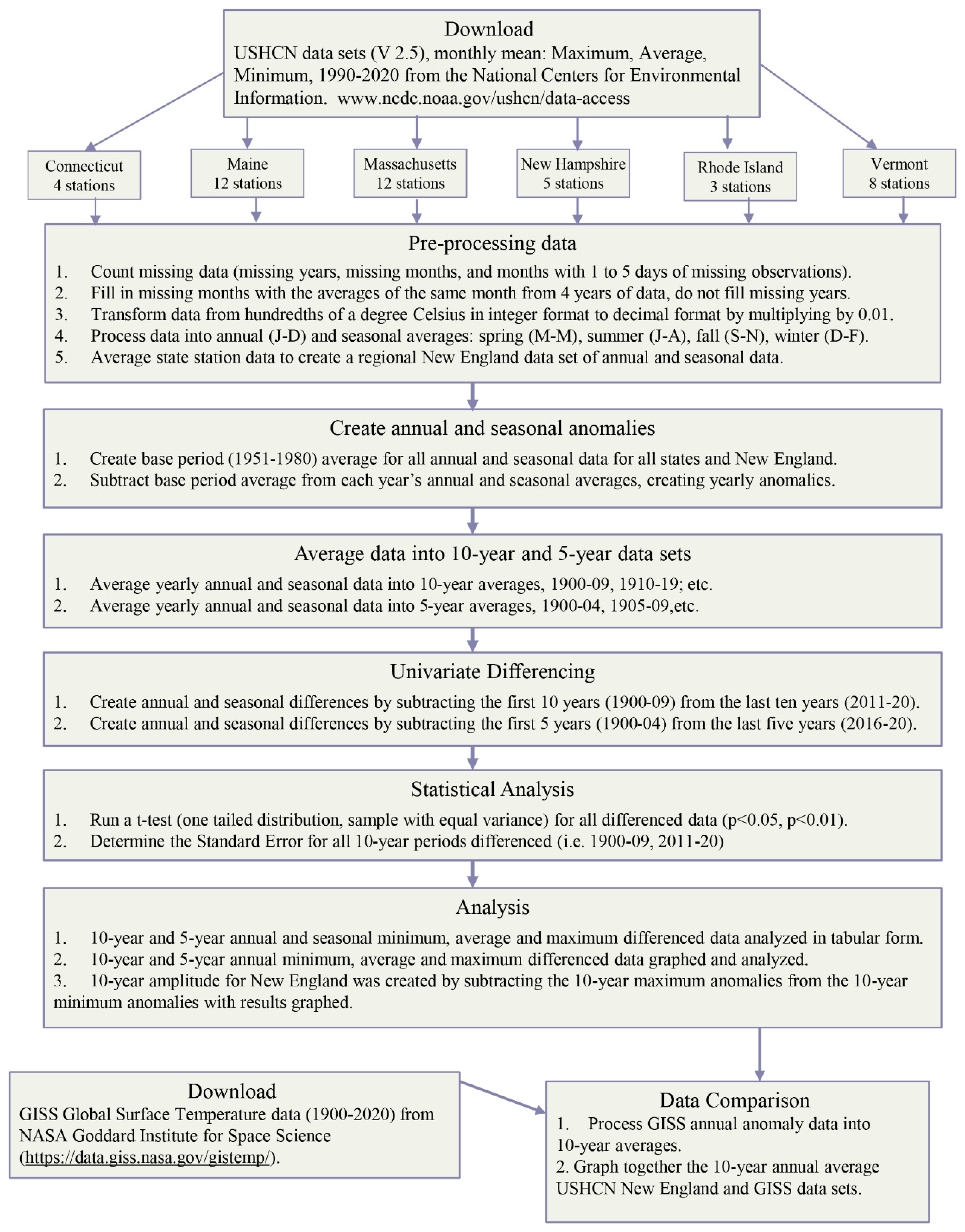
This research analyzed temperature change (minimum, mean, and maximum) between 1900 and 2020 for all New England states and the entire region as a whole for annual and seasonal temperatures. Although some station data start as far back as 1885, 1900 was chosen as a starting date so that most stations would have starting data. Over 77% of the stations in New England have data for 1900 and beyond. Because annual data vary from year to year, and one extreme year can highly skew the data, the data were averaged into five-year and 10-year units. The five-year and 10-year data units were graphed over time as well as differenced. Single-year data were not differenced because of the greater variability of single year of data. Figure 1 outlines the methodology of this research.
Air temperature change is analyzed using the USHCN data set (Version 2.5). Three air temperature data sets (monthly mean minimum, monthly mean average, and monthly mean maximum) were downloaded from the National Centers for Environmental Information (formerly the National Climate Data Center) website (https://www.ncdc.noaa.gov/ushcn/data-access last accessed 6 September 2021). The USHCN stations have been adjusted over time to take into account the validity of extreme outliners, time of observation bias, changes in instrumentations, random relocations of stations, and urban warming biases [35]. Menne et al. (2000) [36] analyzed poorly-sited USHCN stations with good-sited stations and found that adjustments applied to USHCN Version 2 data largely account for the impact of instrument and siting changes. Menne et al. (2010) do note that the adjusted data should not be considered to be completely free from error [36]. However, for New England, Hayhoe et al. (2007) state that the USHCN station data are the best available data for investigating changes since 1900, as the stations have been selected based on the quality and length of data collection and have undergone numerous quality adjustments and validations [31]. In our analysis the quality of the New England USHCN station data were reviewed using the Mann–Kendall Test [37,38,39] and the standard normal homogeneity test [40,41] (details below).
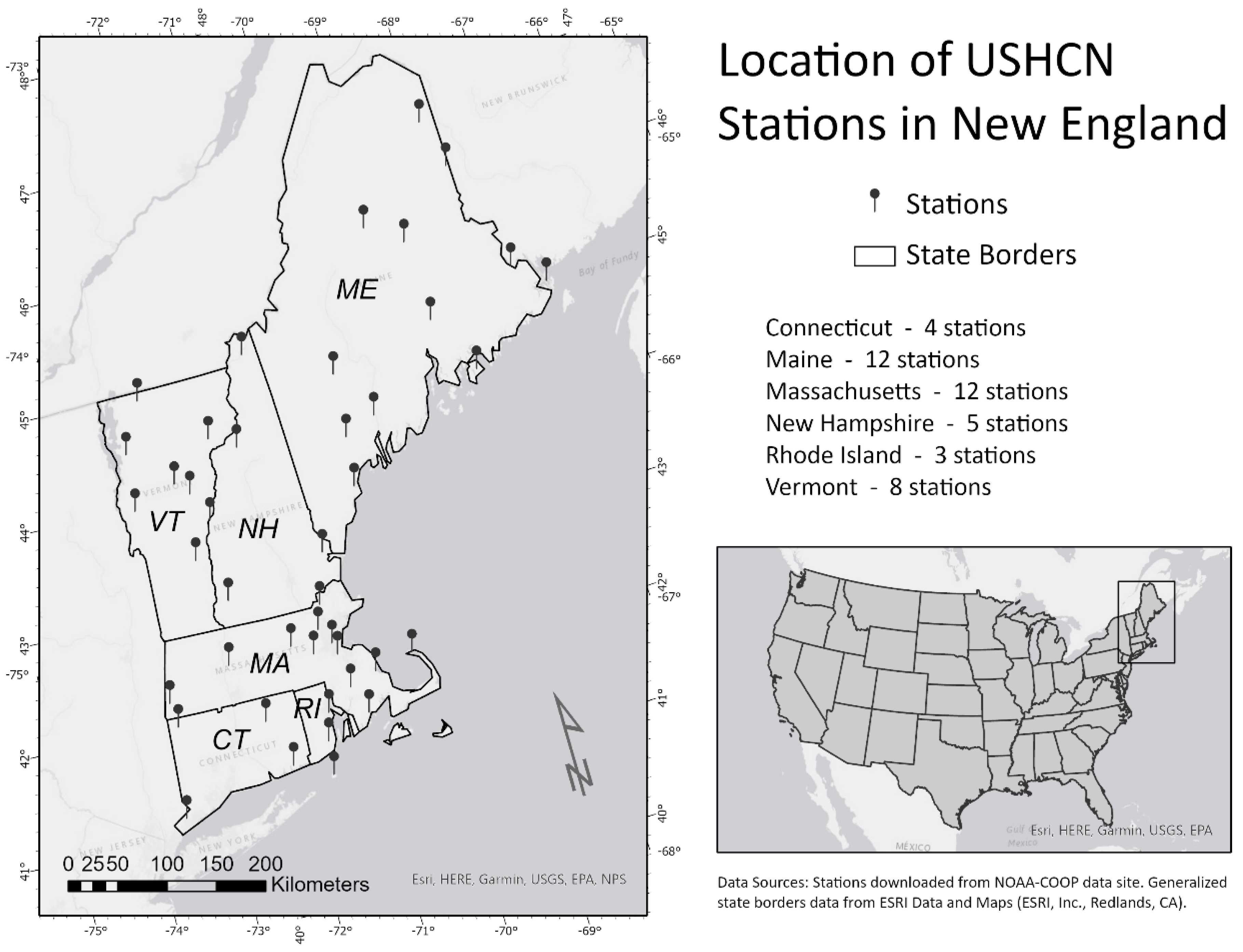
There are 44 USHCN stations in New England: Connecticut (CT) (four stations), Maine (ME) (12 stations), Massachusetts (MA) (12 stations), New Hampshire (NH) (five stations), Rhode Island (RI) (three stations), and Vermont (VT) (eight stations) (Figure 2). Not all of the stations have a complete set of data from 1900 to 2020. The total percentage of missing years for the whole region is 6.7% of the total potential years. For monthly data, 10.8% of data are missing one to five days of observations per month and 2.8% lack six or more days of observation per month.
The three air temperature data sets (minimum, average, and maximum) for the six New England states were downloaded and imported into Microsoft Excel. The data were in monthly mean format for each year. The climate data had four issues that required preprocessing (some stations had missing years of data, some years were missing monthly data, some monthly means were missing days of observations, and data were in integer format in hundredths of degrees Celsius). If a station had a missing year of data, we skipped that year and did not process anything for that year (6.7% of years were missing from the entire data set). For some months, there were one to five days of missing observations for the monthly means (10.8% of total months of the entire data set). In this study, we tolerated one to five missing days of observations per month and used these values with the other monthly means. If there were more than five days of missing observations in a month, then the missing data value (−9999) was a placeholder in the USHCN data. We filled these months with averages for that month determined from two years before and two years after the missing data. If one of the two months before or after were missing, we moved on to the nearest year for that month. Moreover, 2.8% of total months of the entire data set had missing months that were replaced with averages. With so few months and years missing, our averaging of replacement months and skipping of missing years should have a minor influence on the analysis. No state had a disproportionate amount of averaged or missing data. Temperature values were in hundredths of a degree Celsius and were in integer format. The data were converted into decimal format by multiplying each number by 0.01. All data preprocessing was done using the python programming language.
Once the data were preprocessed, annual, and seasonal (spring, summer, fall, winter) averages and anomalies were created from the following months:
- Annual (January, February, March, April, May, June, July, August, September, October, November, December).
- Spring (March, April, May).
- Summer (June, July, August).
- Fall (September, October, November).
- Winter (December of previous year, January of current year, February of current year).
Various researchers have organized USHCN data and other temperature data sets in annual and seasonal formats specifically to reduce noise and provide a clearer signal [42,43,44]. We further reduced the noise by creating five-year and 10-year averages for the annual and seasonal data as others have done [34,45,46].
The annual and seasonal anomalies were created using the 30-year base period of 1951–1980 [47], which is near the middle of the analyzed time period. For every station’s data set, a long-term average (based on the 30-year period: 1951–1980) was created for the annual and seasonal data. The yearly anomalies were created by subtracting the long-term average from each of the yearly annual and seasonal data. The annual and seasonal anomalies from each state were averaged, providing data for all of New England. The annual and seasonal anomalies from every station for every year were then averaged into five-year (half-decade) and 10-year (decadal) data sets. The annual and seasonal data at the five-year and 10-year levels were then graphed and analyzed. Change over time for the annual and seasonal data were analyzed at the five-year and 10-year levels using a univariate differencing method [48] by subtracting the first five years (1900–1904) from the last five years (2016–2020) and the first 10 years (1900–1909) from the last 10 years (2011–2020). Decadal temperature trends in India have been analyzed with a similar univariate differencing method [46]. The differencing was done at the state and New England regional levels. After the differencing, a t-test (one tailed distribution, sample with equal variance) was run for every result to determine if it was significant at the 95th (p < 0.05) or 99th (p < 0.01) percentile. Annual change (2020 minus 1900) was not analyzed because one year can vary greatly and skew the results. For example, for all of New England at the annual average level, 2020 minus 1900 = +1.87 °C, while 2019 minus 1900 = +0.56 °C. The five-year and 10-year averages reduce the annual variability and the t-tests indicate significance. The standard error was determined and graphed for all analyses and in Appendix A, the standard errors of all decades used in the univariate differencing are presented.
To analyze the quality of the USHCN data, the Mann–Kendall Test (significance level set at 5%) was run on each of the 44 USHCN stations’ minimum, average, and maximum annual data as well as on each state’s, and New England’s, minimum, average, and maximum annual and seasonal data. The Mann–Kendall Test is a non-parametric test, which has no prerequisite conditions on the data to be normally distributed [39]. For the test, a null hypothesis (Ho) indicates that there is no trend; the data are independent and random while the alternative hypothesis (Ha) supposes that there is a trend. The standard normal homogeneity test (significance level set at 5%) was also run on the 44 USCHN stations’ annual data. For this test the null hypothesis (Ho) states that the data are homogeneous while the alternative hypothesis (Ha) indicates that there is a change in the data. When the p-value is lower than the 5% significance level, one should reject Ho and accept Ha [40,41,49]. The standard normal homogeneity test can determine where there are non-homogenous breaks in the time series. Concerning sudden changes in the USHCN station data there are a number of possible climatic and non-climatic reasons. One issue about abrupt changes in the USHCN data concerns the replacement of liquid-in-glass thermometers with electronic thermometers at the USHCN sites. To evaluate this potential external force, the changing of thermometers at all 44 stations was investigated and if the timing of the changes occurred at the breaking point indicated by the standard normal homogeneity test, then this potential external error was noted.
The decadal air temperature amplitude of New England’s annual minimum and maximum temperature change was created by subtracting the 10-year maximum anomalies from the 10-year minimum anomalies. If values increase, the minimum temperatures are rising fastest and if the trend declines then the maximum values are increasing faster. The GISS Global Surface Temperature data (in monthly and annual means) were downloaded for the years 1900 to 2020 from the NASA Goddard Institute for Space Science (https://data.giss.nasa.gov/gistemp/ last accessed 6 September 2021). The data came in anomaly format, which used the 1951–1980 base period, the same base period for which we processed the USHCN data [47]. The GISS data were graphed along with the USHCN data to see how New England’s temperature is changing compared with the global temperature change.
3. Results
The results show four broad trends (Table 1 and Table 2, Figure 3 and Figure 4). First, New England as a whole, and each of the states (annually and seasonally), have warmed considerably between 1900 and 2020, with a strong warming trend since the 1960s. Second, for all of the states and the region as a whole, there are three general periods of change: warming from 1900 to the 1950s, cooling into the 1960s, and then warming through to the 2010s. Third, the season experiencing the greatest warming is the winter season, with some states warming more than 3 °C (p < 0.01) based on the 10-year analysis, and some states warming more than 4 °C (p < 0.01) based on the five-year analysis. Fourth, the minimum temperatures are generally warming more than the average and maximum temperatures, especially since the 1980s.
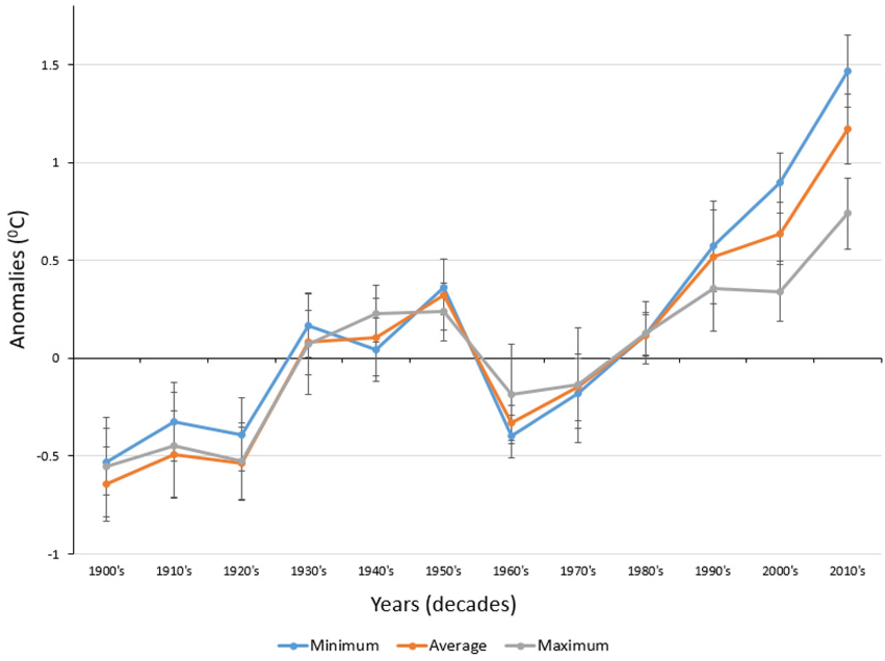
For the 10-year (decadal) temperature change (Table 1, Figure 3), 97% of the differencing results were significant at the 95th percentile (p < 0.05), and 82% were significant at the 99th percentile (p < 0.01). The average and minimum annual temperatures for every state, and New England have increased greater than 1.5 °C with all values being significant (p < 0.01), and most of the minimums increased greater than 2 °C. Concerning the seasons, winter warmed the greatest followed by the summer, fall and spring. For the winter, the average winter temperature change was greater than 2 °C for New England and all six states with all values being significant (p < 0.01). Connecticut’s winter warmed the most with more than a 3 °C increase. The summer and fall seasons warmed in a similar fashion with spring warming the least. For the summer season, the average temperature changed greater than 1.5 °C for New England and all states, except Maine and Vermont, with all values significant (p < 0.01). For every data point (maximum, average, minimum) all spring temperature changes were less than those of the other seasons, except for Vermont and New Hampshire’s maximum spring temperature change. The significance of the spring values were generally lower than the other seasons with the three insignificant figures for the decadal data all occurring in the spring. For the change analysis, there were a total of 105 data points (four seasons and the annual average for six states plus the New England region at the minimum, average, and maximum levels of temperature change, 5 × 7 × 3 = 105). At the decadal level, there was not a single data point that showed a decline in temperature, and 69 out of 105 data points showed an increase of temperature greater than 1.5 °C (66% of points greater than 1.5 °C) and 28 data points greater than 2 °C (27%). All data points greater than 1.5 °C were significant (p < 0.05). For most data points, especially annually and winter, the minimum temperatures increased faster than the average and maximum temperatures, except for Rhode Island, where the maximum temperatures increased the fastest. For the New England region, since the 1990s the minimum temperatures have been increasing significantly faster than the maximum values (Figure 3). The air temperature amplitude of New England’s annual minimum and maximum temperature change shows that since the 1980s the minimum temperature anomalies have been increasing rapidly compared to the maximum temperature anomalies (Figure 5). This shows that annually in New England the minimum temperatures are rising faster than the maximum temperatures.
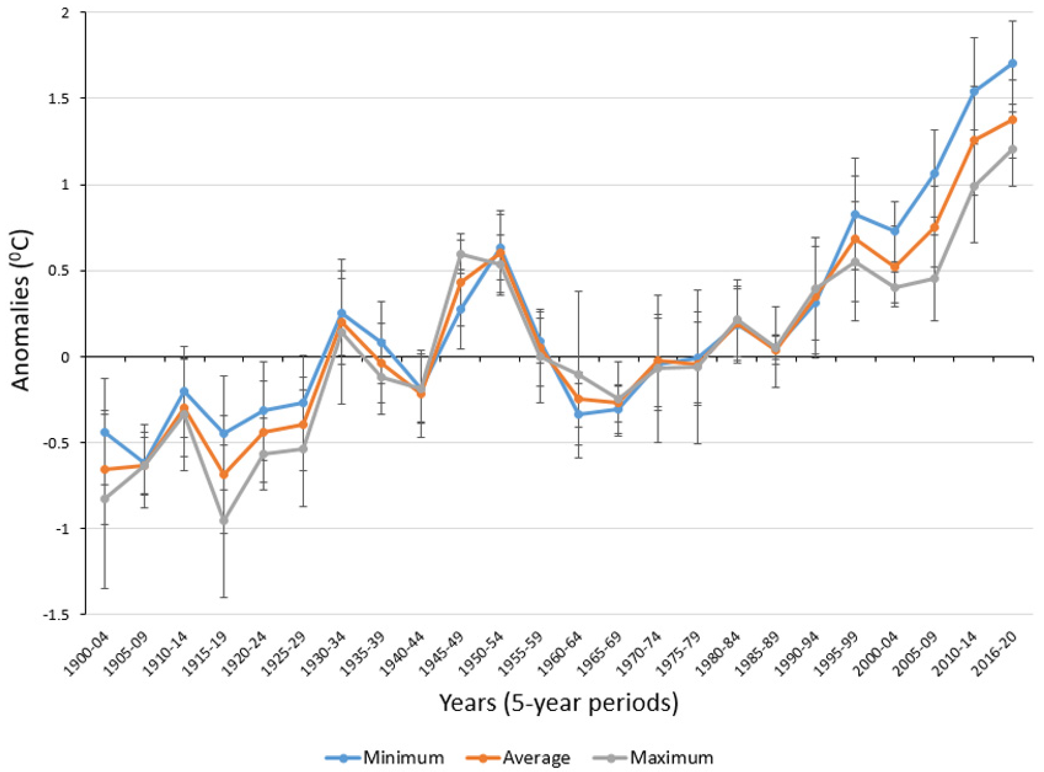
The five-year data analysis (Table 2, Figure 4) showed similar results as the 10-year analysis. However, the significance level for the results of the five-year analysis was lower than for the 10-year analysis. Moreover, 74% of the results were significant at the 95th percentile and 57% at the 99th percentile. All of the annual and winter values were significant (p < 0.01). The average annual temperature for New England and every state has increased greater than 1.5 °C, and for the southern three states (Connecticut, Massachusetts, and Rhode Island), average annual temperatures rose more than 2 °C. The annual average temperature change for New England was also almost 2 °C (1.99 °C). Like the 10-year data, the winter season warmed the most followed by the summer, fall, and spring. For the winter, the average temperature change was greater than 3 °C for all states and New England, with Connecticut warming the most at 4.73 °C. All of the spring values except for Connecticut’s minimum were insignificant, making up 74% of the insignificant values. Like the 10-year results, for most data points, the minimum values were greater than the average and maximum, except for Rhode Island where the maximum values were the highest for all categories.
When looking at the temperature change (minimum, average, and maximum) for New England over the course of the 1900–2020 time period (Figure 3 and Figure 4), there are three general periods of change: warming (1900–1950s), cooling (1950s–1960s), and warming again (1960s–2020). The cooling period appears in the middle of the entire time frame (1900–2020) and divides the changes into two periods of warming. Decadal average annual anomalies reached a peak in the 1950s (0.33) then dropped to a low in the 1960s (–0.33) before rising again (Figure 3). Concerning the five-year average annual anomalies, temperatures reached a peak in the 1950–1954 period (0.60) and declined to a low in the 1965–1969 period (–0.27) before rising again (Figure 4). The minimum, average, and maximum temperature changes at the state levels reflect those of the New England region (Figure 6).
Concerning data for the entire New England region, we used this inflection point of the 1950s to divide the decadal time period into two 60-year warming periods, from the low of 1900 to the warming peak of 1950s and from the low point of the 1960s to the peak of 2010s (Table 3). These two warming periods were similar, as the winter season warmed the most and the spring season the least. However, the second warming period warmed more than the first. As a percentage of the complete period (1900–2020), the second warming period (1960–2020) accounted for more than 70% of the warming for every season and the annual period except for the summer maximum, which was 49%. Only 8 out of 15 values for the first warming period were significant at the 95th percentile, while for the second warming period, 14 out of 15 values were significant at the 95th percentile, and 13 were significant at the 99th percentile.
Concerning the quality of the USHCN data, the results of the Mann–Kendall Test and the standard normal homogeneity test shows that there are some potential errors in the data and that they may be reducing the amount of warming shown in the results. The Mann–Kendall Test for the 44 stations shows that 25% of the minimum, 14% of the average, and 29% of the maximum station data are not significant (5% level) (Table 4). When the insignificant station data are removed from the 10-year and five-year annual data analysis, values for some states increased and others decreased, and for the entire New England region, maximum values increased by 8 to 9% and minimum values rose by 9 to 11% while average values remained almost the same (Table 5). Using all 44 station data, creating annual and seasonal data sets for all states, and New England at the yearly level, the Mann–Kendal analysis only found one data set, Rhode Island’s minimum fall data to be insignificant (Table 6). Thus, the combination of all station data did not create multiple insignificant data sets.
The standard normal homogeneity test run on all 44 station’s minimum and maximum data sets showed that 84 out of 88 data sets were non-homogeneous with specific breaking points (Table 7). Of the 84 data sets with breaking points, 6 had breaking points where new thermometers were replaced (Table 7). Eight of the forty-four stations did not have information about the dates of thermometer changes. Removing these six potentially problematic data sets from the 10-year and five-year annual change analysis created some changes at the state level, but at the New England regional level, changes were less than 2% (Table 8).
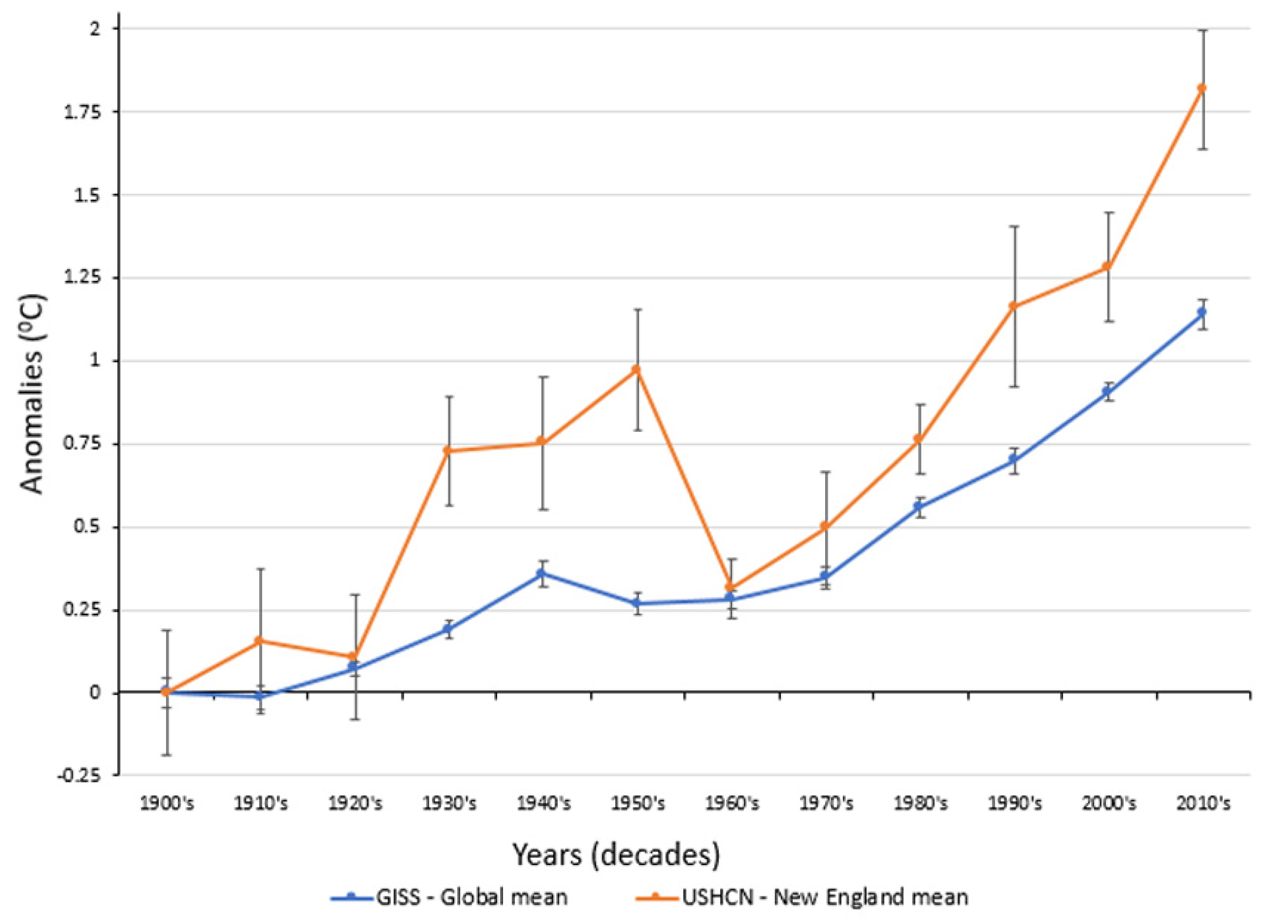
It is clear from this analysis that the New England region is warming in a way similar to much of the world, with an early warming period followed by a brief cooling period and then a return to a warming pattern (Figure 7). New England experienced a greater early rise and a sharper decline than that experienced across the globe. The graph also clearly shows that since the 1960s, New England is warming faster than the world as a whole (Figure 7). The pronounced cooling from the early 1950s through the 1960s is due to the cooling effect of atmospheric aerosols at the global scale, primarily due to human-caused air pollution [50]. The US experienced a greater cooling than the globe as a whole where between the 1930s and 1970s the US cooled 0.5 °C compared to the global cooling of 0.1 °C (48). This mid-century cooling period due to human-caused air pollution has extended longer in parts of Asia such as in northeast India, which had cooling periods due to air pollution into the 2000s [46].
4. Discussion
New England appears to be warming faster than the world as a whole. It is clear from the research that New England has warmed past the 1.5 °C level, which the IPCC has set as a do-not-pass threshold for the world [5], and New England is close to passing the 2 °C level. Regions in the higher latitudes, such as New England, are generally warming faster than the world as a whole. It is also clear from the research that, over the past few decades, the colder temperatures (minimum temperatures and winter temperatures) are warming the fastest. This might be a reason why people in New England are not as aware, or are not as concerned, about the warming temperatures, as they would be if the hottest (maximum and summer season) temperatures were warming the fastest. The warming of the cold temperatures reduces negative effects on human thermal comfort whereas if the hottest temperatures warmed faster, it would create more stress on people’s thermal comfort [51]. The warming of the winter season found in this research reinforces earlier works, which found similar results [18,24,25,26,27,28,30,32,33]. In addition to the air temperatures in New England warming faster than much of the world, the neighboring Gulf of Maine is warming faster than most other ocean water bodies [52].
New England’s rising temperatures are diminishing the distinct seasonality of the region by vastly reducing winter’s cold temperatures as well as increasing temperatures in all of the other seasons. The differences between the four seasons is decreasing. Rising temperatures have resulted in a change in snow cover in the winter. Every decade between 1965 and 2005, New England has lost nine snow-cover days due to less precipitation falling as snow and from the snow melting faster [30]. The loss of snow cover days is occurring throughout much of northeastern North America [53]. Shorter, milder winters will present a variety of challenges for rural industries such as logging, maple syrup harvesting, and the ski industry. Poor road conditions and washouts along with unfrozen forest floors have the potential to limit future logging operations, which need frozen or snow-covered soils [54]. Decreasing snow cover days and warmer winter temperatures are creating the closure of smaller ski areas and driving up the costs at large ski areas [55].
In addition to a loss of snow cover days, warmer winters with rising minimum temperatures will allow insect pests to survive in areas where they could not in the past. Tree pests such as the hemlock woolly adelgid and emerald ash borer have expanded their ranges in New England due to the warmer winters [56,57]. Concerning the spring season, an increase in temperature will shift spring’s seasonal time period (beginning and ending earlier) and affect its seasonal environment. Changes to spring temperatures will have a ripple effect on different species. Biologically, the start of spring is measured by the dates of when leaves and blooms are present on diverse species, which is connected to temperature. As spring temperatures start earlier, so blooms, leaves, and insects will arrive earlier as well. This will affect the insect-eating birds, whose migration is connected to the length of day and not as much on temperature. If the insect population has already peaked when the birds arrive, the birds will not have adequate food sources [58,59]. The late winter, early spring maple syrup season is now in flux with changing temperatures with a threat to the viability of the industry in parts of New England [60].
Summer’s temperatures are increasing and they are expected to continue to increase with more days above 32.2 °C (90° F) [18]. As temperatures increase, the summer season will become lengthier in New England. Summer in New Hampshire is projected to start three weeks earlier and last three more weeks into the fall season [61]. In New England, the number of summer droughts are expected to rise due to earlier snowmelt and more runoff from heavier summer rainfall combined with increased evaporation [62]. Concerning the fall season, with both summer and winter temperatures warming, the fall season will arrive later and extend further. Increasing temperatures will potentially cause New England trees to become drought-stressed, which will change their autumn colors. This would have a negative effect on the fall tourists industry [63].
One outlier in the New England analysis concerns Rhode Island, which is different from all of the other states when considering changes in minimum, average, and maximum temperatures. For New England as a whole and all states except for Rhode Island, the minimum temperatures are rising faster than the average temperatures, which are then rising faster than the maximum temperatures. For Rhode Island, the maximum temperatures are rising faster than the average and the minimum. There are a few possible reasons for this. One is that Rhode Island only had three stations and so the state’s data may be strongly influenced by one or two stations. The USHCN station on Block Island had a particularly strong increase in maximum temperatures relative to the average and minimum temperatures. The three Rhode Island stations are near the ocean and could be influenced by the Long Island Sound. Future research should look at coastal stations in New England outside of Rhode Island to see if there is a similar pattern. It would also be interesting to see if the coastal stations of Maine have warmed due to the warming of the Gulf of Maine.
Although the USHCN is the best data set to analyze long-term temperature change in New England [31], there are some concerns about the quality of the temperature data. The USHCN data set has many stations across the country that have been collecting temperature data for a long time, some for more than 130 years. Over that time span some stations moved their instruments, changed the types of instruments used, changed the times that they made observations and for some places the land cover around the station changed, such as increasing urban environments. The USHCN data has been processed to remove as many of the inconsistencies as possible [35,36]. One inconsistency for the past 70 years or so is a residual maximum temperature bias where USHCN stations underestimate maximum (and mean) temperature trends [64]. So some of the disparity between the minimum and maximum temperatures found in this research might be due to this bias apparently still in the USHCN data. Another bias of concern is from built-environment encroachment near stations, which can artificially increase temperature readings [65]. In this paper the USHCN data for New England was analyzed with the Mann–Kendall Test and the standard normal homogeneity test with results indicating that there may be some issues with a few of the station time series. The potentially problematic data sets were removed from the analysis and compared with the use of all station data. These comparisons indicate that the problematic station data might be lowering the values showing change. Future research needs to be undertaken to analyze the USHCN data for New England in more detail. This analysis of the region used all USHCN station data so that it can be comparable with other USHCN data studies and to be more conservative with the results, as removing stations tended to increase the warming values. Although there may be some issues with a few of the USHCN stations in New England, the overall USHCN observations in New England fall in line with the sheer number of other indicators, such as earlier lake ice-out dates, decreasing snow cover days, the blooming of plants earlier and earlier, or the increasing number of extreme heat events and heat waves with decreasing extreme cold events and cold waves.
Temperatures in New England will not return to where they were a century ago, or even stay where they are now. One of the fundamentals of our current climate is that the temperatures are no longer stable over long periods of time (decades), but they are changing in a warming trend as the data here show. Our world will continue to warm for some time to come. The hope has been to prevent global temperatures from increasing more than 1.5 °C since the start of the Industrial Revolution [5], to avoid the devastating effects of higher seas, more powerful storms, more droughts, increased flooding, more frequent heat waves, and more fires to name some of the consequences that we are now starting to witness due to our warmer world. A warming world will bring a number of positive (or reinforcing) feedbacks, such as melting more snow and ice reducing the reflection of sunlight and increasing the absorption of solar energy making the world even warmer, which then melts more snow and continues the warming. This is now happening in New England and Northeast North America [53]. This, and other positive feedback scenarios, may potentially accelerate warming across the globe in addition to the warming caused by the continuing, increasing concentration of greenhouse gasses such as carbon dioxide [3]. The increasing global greenhouse gasses and positive feedback loops will continue to warm New England and diminish New England’s distinctive four-season climate.
The results of this research have shown areas in need of future research. The influence of the ocean on the temperature data needs to be investigated by examining near-ocean stations and in-land stations to see if there are significant differences between these two sets of stations on the seasonal and annual data. The amplitude of summer vs. winter should be investigated to determine how these two seasons are changing. The amplitude of seasonal maximum and minimum temperatures at the state level needs to be examined. The reasons for various shifts in temperature change at the regional and state levels should be studied, such as the influence of the North Atlantic Oscillation (NAO) on temperatures in New England. Finally, the quality of the USHCN station data for New England needs to be investigated more deeply than we did here.
5. Conclusions
This research clearly shows that New England is warming faster than the world average temperature change, with every season experiencing a warming trend. Winters are warming the fastest followed by the summer, fall, and spring seasons. In addition to the winters warming the fastest, the minimum temperatures across the region are warming faster than the average and maximum temperatures, except for Rhode Island where the maximum temperatures are warming the fastest. The result of this warming is diminishing New England’s distinctive four-season climate, which will alter the ecology of the region as well as having a negative economic impact, especially for outdoor sports, tourism, and biological natural resource-based economies. The changing climate not only alters the ecology and upends the livelihood of many in New England, it also threatens various infrastructures in New England as well the health and well-being of people through more extreme weather, warmer temperatures, floods and droughts, degradation of air and water quality, expansion of diseases, and sea-level rise.
Based on the data presented here, and the continuing increase of greenhouse gases, it is clear that humanity does not have its hand on the rudder of climate control. It is clear from both the 10-year and five-year analysis that New England’s temperature does not show signs of bending towards equilibrium. The science is clear: we are in a climate crisis and we need to take concerted steps to reduce our production of greenhouse gasses as soon as possible. The temperature changes that are currently happening in New England, as outlined in this paper, threaten to disrupt the seasonality of New England, which will disrupt the ecosystems and the economy of New England.
Author Contributions
Conceptualization, S.S.Y.; methodology, S.S.Y.; data pre-processing J.S.Y.; validation, S.S.Y. and J.S.Y.; formal analysis, S.S.Y. and J.S.Y.; writing—original draft preparation, S.S.Y.; writing—review and editing, S.S.Y. and J.S.Y.; visualization, S.S.Y. and J.S.Y. All authors have read and agreed to the published version of the manuscript.
Funding
This research received no external funding.
Data Availability Statement
All data are available in the public domain. Data can be downloaded from the National Centers for Environmental Information (formerly the National Climate Data Center) website (https://www.ncdc.noaa.gov/ushcn/data-access last accessed 6 September 2021). Processed data may be provided upon reasonable request from the authors. GISS data are available from the NASA Goddard Institute for Space Science (https://data.giss.nasa.gov/gistemp/ last accessed 6 September 2021).
Acknowledgments
We would like to acknowledge NOAA and the National Centers for Environmental Information Data for providing access to the USHCH data set and the NASA Goddard Institute for Space Science for providing the global GISS data. We acknowledge the help of colleagues Marcos Luna and Tara Gallagher from Salem State University. This research was supported by the School of Graduate Studies, the Sustainability and Geography department and the Digital Geography Lab at Salem State University.
Conflicts of Interest
The authors declare no competing interests.
Appendix A

Table A1.
Means and Standard Errors in Degrees Celsius for Decades Used to Analyze Temperature Change.
Table A1.
Means and Standard Errors in Degrees Celsius for Decades Used to Analyze Temperature Change.
| State | Annual a | Spring b | Summer c | Fall d | Winter e |
|---|---|---|---|---|---|
| Connecticut | |||||
| (4 USHCN stations) | |||||
| Tmax1900–09 (Mean, Stand. Error) | −0.49, 0.17 | −0.20, 0.29 | −0.24, 0.31 | −0.61, 0.22 | 0.84,0.42 |
| Tmax2011–20 (Mean, Stand. Error) | 0.59, 0.14 | 0.37, 0.28 | 0.45, 0.10 | 0.39, 0.24 | 1.08, 0.45 |
| Tmean1900–09 (Mean, Stand. Error) | −0.70, 0.21 | −0.38, 0.34 | −0.39, 0.37 | −0.69, 0.30 | −1.34, 0.58 |
| Tmean2011–20 (Mean, Stand. Error) | 1.21, 0.18 | 0.85, 0.27 | 1.13, 0.15 | 1.06, 0.28 | 1.79, 0.63 |
| Tmin1900–09 (Mean, Stand. Error) | −0.76, 0.20 | −0.49, 0.35 | −0.48, 0.35 | −0.50, 0.34 | −1.56, 0.60 |
| Tmin2011–20 (Mean, Stand. Error) | 1.68, 0.24 | 1.28, 0.31 | 1.70, 0.20 | 1.58, 0.30 | 2.14, 0.67 |
| Maine | |||||
| (12 USHCN stations) | |||||
| Tmax1900–09 (Mean, Stand. Error) | −0.37, 0.24 | −0.31, 0.40 | −0.44, 0.36 | 0.02, 0.37 | −0.74, 0.60 |
| Tmax2011–20 (Mean, Stand. Error) | 0.84, 0.18 | 0.57, 0.36 | 0.55, 0.16 | 1.07, 0.38 | 1.10, 0.51 |
| Tmean1900–09 (Mean, Stand. Error) | −0.52, 0.21 | −0.38, 0.38 | −0.42, 0.29 | −0.13, 0.31 | −1.12, 0.64 |
| Tmean2011–20 (Mean, Stand. Error) | 1.19, 0.19 | 0.72, 0.33 | 1.04, 0.14 | 1,28, 0.30 | 1.61, 0.57 |
| Tmin1900–09 (Mean, Stand. Error) | −0.66, 0.22 | 0.45, 0.41 | −0.38, 0.26 | −0.28, 0.28 | −1.50, 0.69 |
| Tmin2011–20 (Mean, Stand. Error) | 1.55, 0.20 | 0.91, 0.33 | 1.53, 0.13 | 1.50, 0.25 | 2.18, 0.66 |
| Massachusetts | |||||
| (12 USHCN stations) | |||||
| Tmax1900–09 (Mean, Stand. Error) | −1.05, 0.22 | −0.81, 0.41 | −1.19, 0.38 | −0.99, 0.27 | −1.12, 0.55 |
| Tmax2011–20 (Mean, Stand. Error) | 0.83, 0.20 | 0.52, 0.35 | 0.54, 0.22 | 0.63, 0.35 | 1.51, 0.57 |
| Tmean1900–09 (Mean, Stand. Error) | −0.99, 0.19 | −0.79, 0.30 | −1.10, 0.29 | −0.86, 0.25 | −1.22, 0.53 |
| Tmean2011–20 (Mean, Stand. Error) | 0.97, 0.20 | 0.54, 0.32 | 0.85, 0.19 | 0.80, 0.28 | 1.59, 0.60 |
| Tmin1900–09 (Mean, Stand. Error) | −0.89, 0.17 | −0.61, 0.27 | −0.87, 0.25 | −0.76, 0.25 | −1.35, 0.52 |
| Tmin2011–20 (Mean, Stand. Error) | 1.11, 0.24 | 0.60, 0.34 | 1.16, 0.19 | 0.87, 0.25 | 1.68, 0.67 |
| New Hampshire | |||||
| (5 USHCN stations) | |||||
| Tmax1900–09 (Mean, Stand. Error) | −0.62, 0.23 | −0.64, 0.48 | −0.73, 0.41 | −0.32, 0.37 | −0.71, 0.61 |
| Tmax2011–20 (Mean, Stand. Error) | 0.94, 0.23 | 0.78, 0.40 | 0.81, 0.19 | 0.88, 0.40 | 1.15, 0.56 |
| Tmean1900–09 (Mean, Stand. Error) | −0.55, 0.17 | −0.33, 0.36 | −0.45, 0.24 | −0.47, 0.28 | −0.93, 0.48 |
| Tmean2011–20 (Mean, Stand. Error) | 1.20, 0.20 | 0.80, 0.36 | 1.01, 0.16 | 1.16, 0.28 | 1.67, 0.61 |
| Tmin1900–09 (Mean, Stand. Error) | −0.55, 0.17 | −0.33, 0.36 | −0.45, 0.24 | −0.47, 0.28 | −0.93, 0.48 |
| Tmin2011–20 (Mean, Stand. Error) | 1.48, 0.21 | 0.77, 0.39 | 1.13, 0.16 | 1.45, 0.24 | 2.39, 0.71 |
| Rhode Island | |||||
| (3 USHCN stations) | |||||
| Tmax1900–09 (Mean, Stand. Error) | −0.50, 0.19 | −0.33, 0.33 | −0.49, 0.27 | −0.32, 0.28 | −0.79, 0.52 |
| Tmax2011–20 (Mean, Stand. Error) | 1.39, 0.20 | 1.12, 0.29 | 1.43, 0.21 | 1.22, 0.31 | 1.63, 0.54 |
| Tmean1900–09 (Mean, Stand. Error) | −0.50, 0.19 | −0.33, 0.33 | −0.49, 0.27 | −0.32, 0.28 | −0.79, 0.52 |
| Tmean2011–20 (Mean, Stand. Error) | 1.33, 0.18 | 0.99, 0.27 | 1.34, 0.20 | 1.23, 0.26 | 1.64, 0.59 |
| Tmin1900–09 (Mean, Stand. Error) | −0.28, 0.15 | −0.09, 0.28 | −0.33, 0.19 | 0.09, 0.21 | −0.79, 0.38 |
| Tmin2011–20 (Mean, Stand. Error) | 1.19, 0.14 | 0.94, 0.26 | 1.18, 0.13 | 1.18, 0.18 | 1.38, 0.41 |
| Vermont | |||||
| (8 USHCN stations) | |||||
| Tmax1900–09 (Mean, Stand. Error) | −1.12, 0.20 | −1.21, 0.47 | −1.26, 0.36 | −0.76, 0.38 | −1.12, 0.60 |
| Tmax2011–20 (Mean, Stand. Error) | 0.73, 0.22 | 0.39, 0.41 | 0.23, 0.20 | 0.82, 0.39 | 1.32, 0.55 |
| Tmean1900–09 (Mean, Stand. Error) | −0.64, 0.17 | −0.58, 0.45 | −0.57, 0.28 | −0.43, 0.31 | −0.92, 0.59 |
| Tmean2011–20 (Mean, Stand. Error) | 1.20, 0.24 | 0.64, 0.41 | 0.81, 0.17 | 1.21, 0.31 | 2.00, 0.69 |
| Tmin1900–09 (Mean, Stand. Error) | −0.03, 0.19 | 0.12, 0.40 | 0.22, 0.28 | 0.02, 0.31 | −0.47, 0.62 |
| Tmin2011–20 (Mean, Stand. Error) | 1.83, 0.24 | 1.00, 0.43 | 1.51, 0.14 | 1.65, 0.27 | 2.85, 0.76 |
| New England | |||||
| (44 USHCN stations) | |||||
| Tmax1900–09 (Mean, Stand. Error) | −0.73, 0.21 | −0.62, 0.39 | −0.75, 0.34 | −0.57, 0.30 | −0.91, 0.54 |
| Tmax2011–20 (Mean, Stand. Error) | 0.89, 0.19 | 0.62, 0.34 | 0.67, 0.17 | 0.84, 0.33 | 1.30, 0.52 |
| Tmean1900–09 (Mean, Stand. Error) | −0.65, 0.19 | −0.48, 0.36 | −0.58, 0.30 | −0.44, 0.29 | −1.04, 0.56 |
| Tmean2011–20 (Mean, Stand. Error) | 1.19, 0.19 | 0.76, 0.31 | 1.03, 0.16 | 1.12, 0.27 | 1.72, 0.60 |
| Tmin1900–09 (Mean, Stand. Error) | −0.53, 0.17 | −0.31, 0.32 | −0.38, 0.25 | −0.32, 0.27 | −1.10, 0.52 |
| Tmin2011–20 (Mean, Stand. Error) | 1.48, 0.19 | 0.92, 0.32 | 1.37, 0.14 | 1.37, 0.22 | 2.10, 0.61 |
a Annual refers to the calendar year (January–December). b Spring refers to meteorological spring (March, April, and May). c Summer refers to meteorological summer (June, July, and August). d Fall refers to meteorological fall (September, October, and November). e Winter refers to meteorological winter (December of prior year plus January and February of current year).
References
- Keeling, C.D.; Bacastow, R.B.; Bainbridge, A.E.; Ekdahl, C.A., Jr.; Guenther, P.R.; Waterman, L.S.; Chin, J.F. Atmospheric carbon dioxide variations at Mauna Loa observatory, Hawaii. Tellus 1976, 28, 538–551. [Google Scholar]
- Cox, P.M.; Betts, R.A.; Jones, C.D.; Spall, S.A.; Totterdell, I.J. Acceleration of global warming due to carbon-cycle feedbacks in a coupled climate model. Nature 2000, 408, 184–187. [Google Scholar] [CrossRef]
- Hansen, J.; Nazarenko, L.; Ruedy, R.; Sato, M.; Willis, J.; Del Genio, A.; Koch, D.; Lacis, A.; Lo, K.; Menon, S.; et al. Earth’s energy imbalance: Confirmation and implications. Science 2005, 308, 1431–1435. [Google Scholar] [CrossRef] [PubMed] [Green Version]
- IPCC (Intergovernmental Panel on Climate Change). Climate Change 2013: The Physical Science Basis. Contribution of Working Group I to the Fifth Assessment Report of the Intergovernmental Panel on Climate Change; Cambridge University Press: Cambridge, UK, 2013; Available online: http://www.ipcc.ch/report/ar5/wg1/#.Uq4U93mA2Ul (accessed on 1 May 2021).
- IPCC (Intergovernmental Panel on Climate Change). Global Warming of 1.5 °C. An IPCC Special Report on the Impacts of Global Warming of 1.5 °C above Pre-Industrial Levels and Related Global Greenhouse Gas Emission Pathways, in the Context of Strengthening the Global Response to the Threat of Climate Change, Sustainable Development, and Efforts to Eradicate Poverty. Masson-Delmotte, V., Zhai, P., Pörtner, H.-O., Roberts, D., Skea, J., Shukla, P.R., Pirani, A., Moufouma-Okia, W., Péan, C., Pidcock, R., et al., Eds.; 2018. Available online: https://www.ipcc.ch/site/assets/uploads/sites/2/2019/06/SR15_Full_Report_High_Res.pdf (accessed on 6 November 2021).
- Hughes, L. Biological consequences of global warming: Is the signal already apparent? Trends Ecol. Evol. 2000, 15, 56–61. [Google Scholar] [CrossRef]
- Karl, T.R.; Melillo, J.M.; Peterson, T.C.; Hassol, S.J. (Eds.) Global Climate Change Impacts in the United States; Cambridge University Press: New York, NY, USA, 2009. [Google Scholar]
- Zickfeld, K.; Solomon, S.; Gilford, D.M. Centuries of thermal sea-level rise due to anthropogenic emissions of short-lived greenhouse gases. Proc. Natl. Acad. Sci. USA 2017, 114, 657–662. [Google Scholar] [CrossRef] [Green Version]
- Forster, P.M.; Maycock, A.C.; McKenna, C.M.; Smith, C.J. Latest climate models confirm need for urgent mitigation. Nat. Clim. Chang. 2020, 10, 7–10. [Google Scholar] [CrossRef]
- Lau, L.C.; Lee, K.T.; Mohamed, A.R. Global warming mitigation and renewable energy policy development from the Kyoto Protocol to the Copenhagen Accord—A comment. Renew. Sustain. Energy Rev. 2012, 16, 5280–5284. [Google Scholar] [CrossRef]
- King, A.D.; Karoly, D.J.; Henley, B.J. Australian climate extremes at 1.5 C and 2 C of global warming. Nat. Clim. Chang. 2017, 7, 412–416. [Google Scholar] [CrossRef]
- Schleussner, C.F.; Rogelj, J.; Schaeffer, M.; Lissner, T.; Licker, R.; Fischer, E.M.; Knutti, R.; Levermann, A.; Frieler, K.; Hare, W. Science and policy characteristics of the Paris Agreement temperature goal. Nat. Clim. Chang. 2016, 6, 827–835. [Google Scholar] [CrossRef] [Green Version]
- Sun, Q.; Miao, C.; Hanel, M.; Borthwick, A.G.; Duan, Q.; Ji, D.; Li, H. Global heat stress on health, wildfires, and agricultural crops under different levels of climate warming. Environ. Int. 2019, 128, 125–136. [Google Scholar] [CrossRef] [PubMed]
- Frölicher, T.L.; Fischer, E.M.; Gruber, N. Marine heatwaves under global warming. Nature 2018, 560, 360–364. [Google Scholar] [CrossRef]
- Karmalkar, A.V.; Bradley, R.S. Consequences of global warming of 1.5 C and 2 C for regional temperature and precipitation changes in the contiguous United States. PLoS ONE 2017, 12, e0168697. [Google Scholar] [CrossRef] [Green Version]
- New England Foliage–Yankee New England. Available online: https://newengland.com/category/seasons/page/5/ (accessed on 26 July 2021).
- New England Regional Assessment Group (NERA). Preparing for a Changing Climate: The Potential Consequences of Climate Variability and Change: New England Regional Overview. In U.S. Global Change Research Program; University of New Hampshire: Durham, NH, USA, 2001; p. 88. [Google Scholar]
- Dupigny-Giroux, L.A.; Mecray, E.; Lemcke-Stampone, M.; Hodgkins, G.A.; Lentz, E.E.; Mills, K.E.; Lane, E.D.; Miller, R.; Hollinger, D.; Solecki, W.D.; et al. Chapter 18: Northeast. In Impacts, Risks, and Adaptation in the United States: The Fourth National Climate Assessment; US Global Change Research Program: Washington, DC, USA, 2018; Volume 2. [Google Scholar]
- Outdoor Industry Association. The Outdoor Recreation Economy; Outdoor Industry Association: Boulder, CO, USA, 2017; p. 19. [Google Scholar]
- Lopez, R.; Plesha, N.; Campbell, B.; Laughton, C. Northeast Economic Engine: Agriculture, Forest Products and Commercial Fishing; Farm Credit East: Enfield, CT, USA, 2015; p. 25. [Google Scholar]
- Becot, F.; Kolodinsky, J.; Conner, D. The Economic Contribution of the Vermont Maple Industry; Center for Rural Studies at the University of Vermont: Burlington, VT, USA, 2015. [Google Scholar]
- Leff, D.K. Maple Sugaring: Keeping it Real in New England; Wesleyan University Press: Middletown, CT, USA, 2015. [Google Scholar]
- Cooter, E.J.; Leduc, S.K. Recent frost date trends in the north-eastern USA. Int. J. Climatol. 1995, 15, 65–75. [Google Scholar] [CrossRef]
- Hodgkins, G.A.; James, I.C.; Huntington, T.G. Historical changes in lake ice-out dates as indicators of climate change in New England, 1850–2000. Int. J. Climatol. J. R. Meteorol. Soc. 2002, 22, 1819–1827. [Google Scholar] [CrossRef]
- Hodgkins, G.A.; Dudley, R.W.; Huntington, T.G. Changes in the timing of high river flows in New England over the 20th century. J. Hydrol. 2003, 278, 244–252. [Google Scholar] [CrossRef] [Green Version]
- Hodgkins, G.A.; Dudley, R.W.; Huntington, T.G. Changes in the number and timing of ice-affected flow days on New England rivers, 1930–2000. Clim. Chang. 2005, 71, 319–340. [Google Scholar] [CrossRef]
- Huntington, T.G.; Hodgkins, G.A.; Keim, B.D.; Dudley, R.W. Changes in the proportion of precipitation occurring as snow in New England (1949–2000). J. Clim. 2004, 17, 2626–2636. [Google Scholar] [CrossRef]
- Wolfe, D.W.; Schwartz, M.D.; Lakso, A.N.; Otsuki, Y.; Pool, R.M.; Shaulis, N.J. Climate change and shifts in spring phenology of three horticultural woody perennials in northeastern USA. Int. J. Biometeorol. 2005, 49, 303–309. [Google Scholar] [CrossRef]
- Trombulak, S.C.; Wolfson, R. Twentieth-century climate change in New England and New York, USA. Geophys. Res. Lett. 2004, 31. [Google Scholar] [CrossRef]
- Burakowski, E.A.; Wake, C.P.; Braswell, B.; Brown, D.P. Trends in wintertime climate in the northeastern United States: 1965–2005. J. Geophys. Res. Atmos. 2008, 113, D20. [Google Scholar] [CrossRef]
- Hayhoe, K.; Wake, C.P.; Huntington, T.G.; Luo, L.; Schwartz, M.D.; Sheffield, J.; Wood, E.; Anderson, B.; Bradbury, J.; DeGaetano, A.; et al. Past and future changes in climate and hydrological indicators in the US Northeast. Clim. Dyn. 2007, 28, 381–407. [Google Scholar] [CrossRef]
- Brown, P.J.; Bradley, R.; Keimig, F. Changes in extreme climate indices for the northeastern United States, 1870–2005. J. Clim. 2010, 23, 6555–6572. [Google Scholar] [CrossRef]
- Thibeault, J.M.; Seth, A. Changing climate extremes in the Northeast United States: Observations and projections from CMIP5. Clim. Chang. 2014, 127, 273–287. [Google Scholar] [CrossRef]
- Runkle, J.; Kunkel, K.E.; Easterling, D.; Stewart, B.C.; Champion, S.; Stevens, L.; Frankson, R.; Sweet, W. State Climate Summaries: Rhode Island; NOAA Technical Report NESDIS 149-RI; NOAA National Centers for Environmental Information: Asheville, NC, USA, 2017; p. 4.
- Keim, B.D.; Wilson, A.M.; Wake, C.P.; Huntington, T.G. Are there spurious temperature trends in the United States Climate Division database? Geophys. Res. Lett. 2003, 30. [Google Scholar] [CrossRef] [Green Version]
- Menne, M.J.; Williams, C.N., Jr.; Palecki, M.A. On the reliability of the US surface temperature record. J. Geophys. Res. Atmos. 2010, 115. [Google Scholar] [CrossRef] [Green Version]
- Kendall, M.G. Rank Correlation Methods; Griffin: London, UK, 1975; ISBN 9780852641996. [Google Scholar]
- Mann, H.B. Nonparametric Tests Against Trend. Econometrica 1945, 13, 245. [Google Scholar] [CrossRef]
- Tabari, H.; Marofi, S.; Aeini, A.; Talaee, P.H.; Mohammadi, K. Trend analysis of reference evapotranspiration in the western half of Iran. Agric. For. Meteorol. 2011, 151, 128–136. [Google Scholar] [CrossRef]
- Alexandersson, H.A. A homogeneity test applied to precipitation data. J. Climatol. 1986, 6, 661–675. [Google Scholar] [CrossRef]
- Alexandersson, H.; Moberg, A. Homogenization of Swedish Temperature Data Part I: Homogeneity Test for Linear Trends. J. Climatol. 1997, 17, 25–34. [Google Scholar] [CrossRef]
- Elagib, N.A.; Mansell, M.G. Recent trends and anomalies in mean seasonal and annual temperatures over Sudan. J. Arid Environ. 2000, 45, 263–288. [Google Scholar] [CrossRef]
- Hulme, M.; Doherty, R.; Ngara, T.; New, M.; Lister, D. African climate change: 1900–2100. Clim. Res. 2001, 17, 145–168. [Google Scholar] [CrossRef] [Green Version]
- Lynch, C.; Seth, A.; Thibeault, J. Recent and projected annual cycles of temperature and precipitation in the Northeast United States from CMIP5. J. Clim. 2016, 29, 347–365. [Google Scholar] [CrossRef]
- Gille, S.T. Decadal-scale temperature trends in the Southern Hemisphere ocean. J. Clim. 2008, 21, 4749–4765. [Google Scholar] [CrossRef]
- Ross, R.S.; Krishnamurti, T.N.; Pattnaik, S.; Pai, D.S. Decadal surface temperature trends in India based on a new high-resolution data set. Sci. Rep. 2018, 8, 7452. [Google Scholar] [CrossRef] [Green Version]
- Hansen, J.; Ruedy, R.; Glascoe, J.; Sato, M. GISS analysis of surface temperature change. J. Geophys. Res. Atmos. 1999, 104, 30997–31022. [Google Scholar] [CrossRef]
- Singh, A. Review article digital change detection techniques using remotely-sensed data. Int. J. Remote Sens. 1989, 10, 989–1003. [Google Scholar] [CrossRef] [Green Version]
- Khaliq, M.N.; Ouarda, T.B. On the critical values of the standard normal homogeneity test (SNHT). Int. J. Climatol. A J. R. Meteorol. Soc. 2007, 27, 681–687. [Google Scholar] [CrossRef]
- Wilcox, L.J.; Highwood, E.J.; Dunstone, N.J. The influence of anthropogenic aerosol on multi-decadal variations of historical global climate. Environ. Res. Lett. 2013, 8, 024033. [Google Scholar] [CrossRef]
- Matzarakis, A.; Amelung, B. Physiological equivalent temperature as indicator for impacts of climate change on thermal comfort of humans. In Seasonal Forecasts, Climatic Change and Human Health; Springer: Dordrecht, The Netherlands, 2008; pp. 161–172. [Google Scholar]
- Poppick, L. Why is the Gulf of Maine warming faster than 99% of the ocean? EOS 2018, 99. [Google Scholar] [CrossRef]
- Thiebault, K.; Young, S. Snow cover change and its relationship with land surface temperature and vegetation in northeastern North America from 2000 to 2017. Int. J. Remote Sens. 2020, 41, 8453–8474. [Google Scholar] [CrossRef]
- Swanston, C.; Brandt, L.A.; Janowiak, M.K.; Handler, S.D.; Butler-Leopold, P.; Iverson, L.; Thompson, F.R., III; Ontl, T.A.; Shannon, P.D. Vulnerability of forests of the Midwest and Northeast United States to climate change. Clim. Chang. 2018, 146, 103–116. [Google Scholar] [CrossRef]
- Beaudin, L.; Huang, J.C. Weather conditions and outdoor recreation: A study of New England ski areas. Ecol. Econ. 2014, 106, 56–68. [Google Scholar] [CrossRef]
- Paradis, A.; Elkinton, J.; Hayhoe, K.; Buonaccorsi, J. Role of winter temperature and climate change on the survival and future range expansion of the hemlock woolly adelgid (Adelges tsugae) in eastern North America. Mitig. Adapt. Strateg. Glob. Chang. 2008, 13, 541–554. [Google Scholar] [CrossRef]
- DeSantis, R.D.; Moser, W.K.; Gormanson, D.D.; Bartlett, M.G.; Vermunt, B. Effects of climate on emerald ash borer mortality and the potential for ash survival in North America. Agric. For. Meteorol. 2013, 178, 120–128. [Google Scholar] [CrossRef]
- Union of Concerned Scientists (UCS). The Changing Northeast Climate; UCS Publications: Cambridge, MA, USA, 2006. [Google Scholar]
- MacKenzie, C.M.; Johnston, J.; Miller-Rushing, A.J.; Sheehan, W.; Pinette, R.; Primack, R. Advancing Leaf-Out and Flowering Phenology is Not Matched by Migratory Bird Arrivals Recorded in Hunting Guide’s Journal in Aroostook County, Maine. Northeast. Nat. 2019, 26, 561–579. [Google Scholar] [CrossRef]
- Skinner, C.B.; DeGaetano, A.T.; Chabot, B.F. Implications of twenty-first century climate change on Northeastern United States maple syrup production: Impacts and adaptations. Clim. Chang. 2010, 100, 685–702. [Google Scholar] [CrossRef]
- Hayhoe, K.; Wake, C.; Anderson, B.; Liang, X.Z.; Maurer, E.; Zhu, J.; Bradbury, J.; DeGaetano, A.; Stoner, A.M.; Wuebbles, D. Regional climate change projections for the Northeast USA. Mitig. Adapt. Strateg. Glob. Chang. 2008, 13, 425–436. [Google Scholar] [CrossRef]
- Betts, A.K. Vermont climate change indicators. Weather Clim. Soc. 2011, 3, 106–115. [Google Scholar] [CrossRef]
- Huntington, T.G.; Richardson, A.D.; McGuire, K.J.; Hayhoe, K. Climate and hydrological changes in the northeastern United States: Recent trends and implications for forested and aquatic ecosystems. Can. J. For. Res. 2009, 39, 199–212. [Google Scholar] [CrossRef] [Green Version]
- Hausfather, Z.; Cowtan, K.; Menne, M.J.; Williams, C.N., Jr. Evaluating the impact of US historical climatology network homogenization using the US climate reference network. Geophys. Res. Lett. 2016, 43, 1695–1701. [Google Scholar] [CrossRef] [Green Version]
- Leeper, R.D.; Kochendorfer, J.; Henderson, T.A.; Palecki, M.A. Impacts of small-scale urban encroachment on air temperature observations. J. Appl. Meteorol. Climatol. 2019, 58, 1369–1380. [Google Scholar] [CrossRef]
Figure 1.
Methodology outline.

Figure 2.
Location map of 44 USHCN stations in New England.

Figure 3.
Decadal temperature anomalies for New England, 1900–2020. (USHCN data for New England temperature anomalies: minimum, average, and maximum. Base period for the production of anomalies = 1951–1980. Error bars based on standard error.).
Figure 3.
Decadal temperature anomalies for New England, 1900–2020. (USHCN data for New England temperature anomalies: minimum, average, and maximum. Base period for the production of anomalies = 1951–1980. Error bars based on standard error.).

Figure 4.
Half-decadal (five-year) temperature anomalies for New England, 1900–2020 (USHCN data Figure 1951. Error bars based on standard error.).
Figure 4.
Half-decadal (five-year) temperature anomalies for New England, 1900–2020 (USHCN data Figure 1951. Error bars based on standard error.).

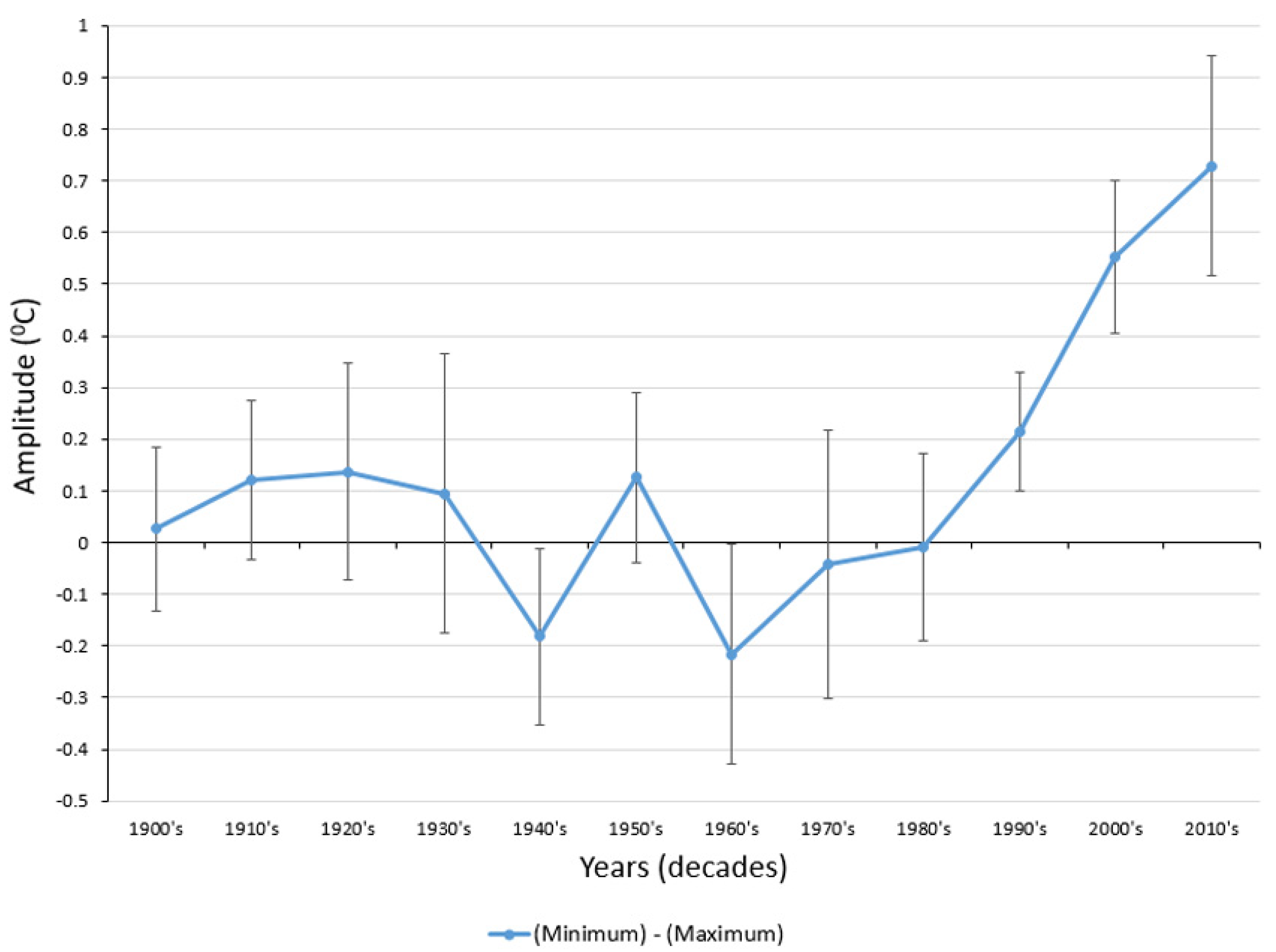
Figure 5.
New England amplitude changes for minimum minus maximum anomalies, 1900–2020. (Graph plots the amplitude of New England’s USHCN minimum anomalies minus maximum anomalies by decade, 1900–2020. Base period for the production of anomalies = 1951–1980. Error bars based on standard error. Decreasing lines indicate maximum values increasing faster than minimum values and rising lines indicate minimum values rising faster than maximum values.).

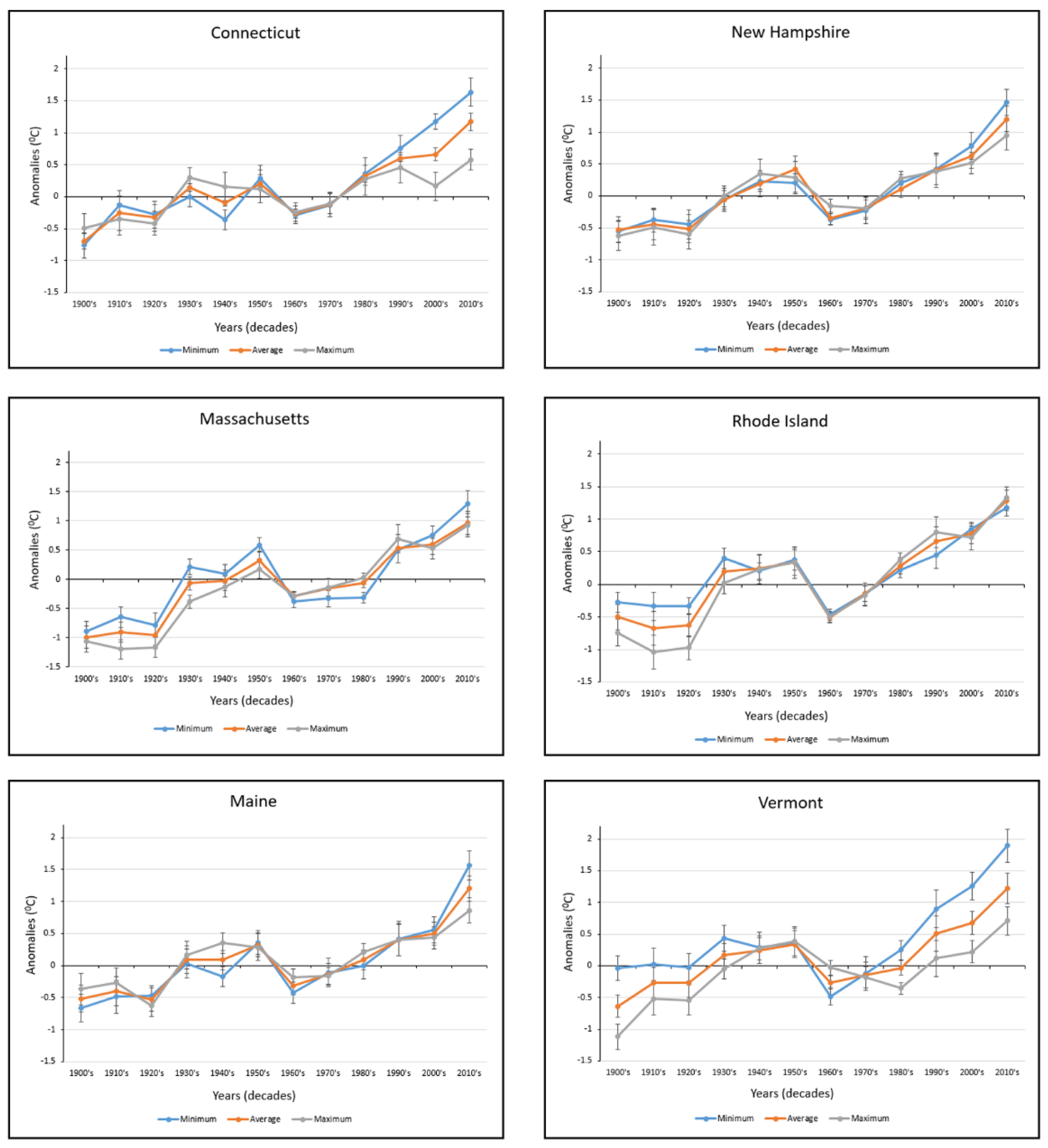
Figure 6.
Decadal temperature anomalies for each state in New England, 1900–2020 (USHCN data for state temperature anomalies: minimum, average, and maximum. Base period for the production of anomalies = 1951–1980. Error bars based on standard error.).
Figure 6.
Decadal temperature anomalies for each state in New England, 1900–2020 (USHCN data for state temperature anomalies: minimum, average, and maximum. Base period for the production of anomalies = 1951–1980. Error bars based on standard error.).

Figure 7.
Decadal temperature anomalies for New England and the World, 1900–2020 (New England data from the USHCN data set. World data from the NASA Goddard Institute for Space Science GISS data set. Both data sets created anomalies from the 1951–1980 base period. Error bars based on standard error. For comparative purposes, starting points for both data sets were calibrated to zero by raising each line by the 1900s anomaly (0.313 for the World and 0.645 for New England)).

Table 1.
New England Decadal Temperature Change Values (2011–2020) minus (1900–1909) in degrees Celsius.
Table 1.
New England Decadal Temperature Change Values (2011–2020) minus (1900–1909) in degrees Celsius.
| State | Annual a | Spring b | Summer c | Fall d | Winter e | Over 1.5 °C f |
|---|---|---|---|---|---|---|
| Connecticut | ||||||
| (4 USHCN stations) | ||||||
| Maximum | 1.08 ** | 0.57 | 0.69 * | 1.00 ** | 1.92 ** | 10/15 |
| Average | 1.91 ** | 1.23 ** | 1.52 ** | 1.68 ** | 3.13 ** | |
| Minimum | 2.44 ** | 1.77 ** | 2.18 ** | 2.08 ** | 3.70 ** | |
| Maine | ||||||
| (12 USHCN stations) | ||||||
| Maximum | 1.21 ** | 0.87 | 0.98 * | 1.05 * | 1.83 * | 7/15 |
| Average | 1.70 ** | 1.10 * | 0.46 ** | 1.41 ** | 2.73 ** | |
| Minimum | 2.21 ** | 1.36 ** | 1.91 ** | 1.78 ** | 3.67 ** | |
| Massachusetts | ||||||
| (12 USHCN stations) | ||||||
| Maximum | 1.88 ** | 1.33 * | 1.73 ** | 1.63 ** | 2.63 ** | 12/15 |
| Average | 1.97 ** | 1.33 ** | 1.94 ** | 1.66 ** | 2.81 ** | |
| Minimum | 2.00 ** | 1.22 ** | 2.03 ** | 1.64 ** | 3.02 ** | |
| New Hampshire | ||||||
| (5 USHCN stations) | ||||||
| Maximum | 1.57 ** | 1.42 * | 1.54 ** | 1.21 * | 1.87 * | 10/15 |
| Average | 1.73 ** | 1.20 * | 1.53 ** | 1.47 ** | 2.50 ** | |
| Minimum | 2.04 ** | 1.10 * | 1.58 ** | 1.92 ** | 3.32 ** | |
| Rhode Island | ||||||
| (3 USHCN stations) | ||||||
| Maximum | 2.13 ** | 1.71 ** | 2.07 ** | 1.96 ** | 2.54 ** | 11/15 |
| Average | 1.83 ** | 1.33 ** | 1.83 ** | 1.55 ** | 2.44 ** | |
| Minimum | 1.47 ** | 1.03 ** | 1.50 ** | 1.09 ** | 2.17 ** | |
| Vermont | ||||||
| (8 USHCN stations) | ||||||
| Maximum | 1.85 ** | 1.60 ** | 1.49 ** | 1.58 ** | 2.44 ** | 10/15 |
| Average | 1.84 ** | 1.22 * | 1.37 ** | 1.64 ** | 2.92 ** | |
| Minimum | 1.87 ** | 0.88 | 1.30 ** | 1.64 ** | 3.33 ** | |
| New England | ||||||
| (44 USHCN stations) | ||||||
| Maximum | 1.62 ** | 1.25 * | 1.42 ** | 1.40 ** | 2.21 ** | 10/15 |
| Average | 1.83 ** | 1.23 ** | 1.61 ** | 1.57 ** | 2.75 ** | |
| Minimum | 2.01 ** | 1.23 * | 1.75 ** | 1.69 ** | 3.20 ** |
a Annual refers to the calendar year (January–December). b Spring refers to meteorological spring (March, April, and May). c Summer refers to meteorological summer (June, July, and August). d Fall refers to meteorological fall (September, October, and November). e Winter refers to meteorological winter (December of prior year plus January and February of current year). f This column shows the number of data points over 1.5 °C for the 15 data points per state: 5 (1 annual + 4 seasons) × 3 (Tmax + Ta + Tmin) = 15. Numbers with Italic font were at 1.5 °C or above. Numbers with Italic font and Bold were at 2 °C or above. * Significant at the 95th percentile (p < 0.05). ** Significant at the 99th percentile (p < 0.01).
Table 2.
New England five-year temperature change values (2016–2020) minus (1900–1904) in degrees Celsius.
Table 2.
New England five-year temperature change values (2016–2020) minus (1900–1904) in degrees Celsius.
| State | Annual a | Spring b | Summer c | Fall d | Winter e | Over 1.5 °C f |
|---|---|---|---|---|---|---|
| Connecticut | ||||||
| (4 USHCN stations) | ||||||
| Maximum | 1.25 ** | 0.21 | 0.73 | 1.08 * | 3.04** | 10/15 |
| Average | 2.32 ** | 0.97 | 1.73 * | 1.89 * | 4.73 ** | |
| Minimum | 2.98 ** | 1.66 ** | 2.50 ** | 2.40 ** | 5.38 ** | |
| Maine | ||||||
| (12 USHCN stations) | ||||||
| Maximum | 1.41 ** | 0.04 | 1.59 * | 1.04 | 2.71 * | 9/15 |
| Average | 1.89 ** | 0.36 | 1.82 ** | 1.48 * | 3.54 ** | |
| Minimum | 2.37 ** | 0.69 | 1.99 ** | 1.94 ** | 4.50 ** | |
| Massachusetts | ||||||
| (12 USHCN stations) | ||||||
| Maximum | 2.05 ** | 0.52 | 2.39 ** | 1.56 * | 3.61 ** | 12/15 |
| Average | 2.16 ** | 0.7 | 2.39 ** | 1.70 * | 3.83 ** | |
| Minimum | 2.29 ** | 0.91 | 2.28 ** | 1.74 ** | 4.26 ** | |
| New Hampshire | ||||||
| (5 USHCN stations) | ||||||
| Maximum | 1.53 ** | 0.25 | 2.09 * | 0.91 | 2.72 * | 10/15 |
| Average | 1.68 ** | 0.3 | 1.70 * | 1.24 | 3.29 ** | |
| Minimum | 2.15 ** | 0.57 | 1.64 ** | 1.91 * | 4.31 ** | |
| Rhode Island | ||||||
| (3 USHCN stations) | ||||||
| Maximum | 2.40 ** | 1.06 | 2.26 ** | 2.17 ** | 3.72 ** | 10/15 |
| Average | 2.06 ** | 0.8 | 2.01 ** | 1.79 * | 3.70 ** | |
| Minimum | 1.48 ** | 0.38 | 1.51 ** | 1.25 ** | 2.73 ** | |
| Vermont | ||||||
| (8 USHCN stations) | ||||||
| Maximum | 1.89 ** | 0.49 | 2.15 ** | 1.41 | 3.27 ** | 8/15 |
| Average | 1.81 ** | 0.23 | 1.67 * | 1.47 * | 3.70 ** | |
| Minimum | 1.62 ** | −0.15 | 1.17 * | 1.36 | 3.77 ** | |
| New England | ||||||
| (44 USHCN stations) | ||||||
| Maximum | 1.76 ** | 0.43 | 1.87 * | 1.36 | 3.18 ** | 12/15 |
| Average | 1.99 ** | 0.56 | 1.89 ** | 1.60 * | 3.80 ** | |
| Minimum | 2.15 ** | 0.68 | 1.85 ** | 1.77 ** | 4.16** |
a Annual refers to the calendar year (January–December). b Spring refers to meteorological spring (March, April, and May). c Summer refers to meteorological summer (June, July, and August). d Fall refers to meteorological fall (September, October, and November). e Winter refers to meteorological winter (December of prior year plus January and February of current year). f This column shows the number of data points over 1.5 °C for the 15 data points per state: 5 (1 annual + 4 seasons) × 3 (Tmax + Ta + Tmin) = 15. Numbers with Italic font were at 1.5 °C or above. Numbers with Italic font and Bold were at 2 °C or above. * Significant at the 95th percentile (p < 0.05). ** Significant at the 99th percentile (p < 0.01).
Table 3.
Changes of decadal temperatures for different time periods in New England in degrees Celsius.
Table 3.
Changes of decadal temperatures for different time periods in New England in degrees Celsius.
| Level | Annual a | Spring b | Summer c | Fall d | Winter e |
|---|---|---|---|---|---|
| Complete Period (2011–2020) minus (1900–1909) | |||||
| Maximum | 1.62 ** | 1.25 * | 1.42 ** | 1.24 ** | 2.01 ** |
| Average | 1.83 ** | 1.23 ** | 1.61 ** | 1.57 * | 2.75 ** |
| Minimum | 2.01 ** | 1.23 * | 1.75 ** | 1.70 * | 3.20** |
| First Warming Period (1950–1959) minus (1900–1909) | |||||
| Maximum | 1.00 ** | 0.56 | 0.74 | 0.88 * | 1.76 ** |
| Average | 0.97 ** | 0.53 | 0.56 | 0.71 * | 2.00 ** |
| Minimum | 0.89 ** | 0.48 | 0.31 | 0.51 | 2.19** |
| Second Warming Period (2011–2020) minus (1960–1969) | |||||
| Maximum | 1.13 ** | 0.87 * | 0.69 ** | 0.9 | 1.64 ** |
| Average | 1.51 ** | 1.08 ** | 1.15 ** | 1.31 ** | 2.10 ** |
| Minimum | 1.88 ** | 1.31 ** | 1.56 ** | 1.63 ** | 2.26** |
| Second Warming Period as a Percent of Complete Period f | |||||
| Maximum | 70% | 70% | 49% | 73% | 82% |
| Average | 83% | 88% | 71% | 83% | 76% |
| Minimum | 94% | 107% | 89% | 96% | 71% |
a Annual refers to the calendar year (January–December). b Spring refers to meteorological spring (March, April, and May). c Summer refers to meteorological summer (June, July, and August). d Fall refers to meteorological fall (September, October, and November). e Winter refers to meteorological winter (December of prior year plus January and February of current year). f Value in the Second Warming Period divided by value in the Complete Period, such as 1.13/1.62 = 70%. Numbers with Italic font were at 1.5 °C or above. Numbers with Italic font and Bold were at 2 °C or above. * Significant at the 95th percentile (p < 0.05). ** Significant at the 99th percentile (p < 0.01).
Table 4.
Mann–Kendal Test for all 44 New England USHCN stations at the 95th percentile.
| State | Station | Tmin | Tmean | Tmax |
|---|---|---|---|---|
| CT | USH00062658 | x | x | |
| MA | USH00190120 | x | ||
| MA | USH00193213 | x | x | |
| MA | USH00196486 | x | ||
| MA | USH00196681 | x | ||
| MA | USH00199316 | x | ||
| ME | USH00170100 | x | ||
| ME | USH00170814 | x | x | x |
| ME | USH00172765 | x | x | |
| ME | USH00173944 | x | ||
| ME | USH00176905 | x | ||
| ME | USH00179891 | x | ||
| NH | USH00270706 | x | ||
| NH | USH00272999 | x | x | x |
| RI | USH00370896 | x | ||
| VT | USH00431243 | x | ||
| VT | USH00431360 | x | x | x |
| VT | USH00431580 | x | ||
| VT | USH00432769 | x | ||
| VT | USH00437607 | x | ||
| VT | USH00437612 | x |
x indicates station data that were not significant at the 95th percentile.
Table 5.
Comparison in degrees Celsius of all USHCN station data vs. only significant station data based on the Mann–Kendall Test for annual anomaly change at the 10-year and five-year levels.
Table 5.
Comparison in degrees Celsius of all USHCN station data vs. only significant station data based on the Mann–Kendall Test for annual anomaly change at the 10-year and five-year levels.
| 10 Year Data | Five Year Data | |||
|---|---|---|---|---|
| State | Full Set a | Selected b | Full Set a | Selected b |
| Connecticut | ||||
| (4 USHCN stations) | ||||
| Maximum | 1.36 | 1.33 | 1.67 | 1.67 |
| Average | 1.91 | 1.91 | 2.32 | 2.32 |
| Minimum | 2.44 | 2.51 | 2.98 | 2.98 |
| Maine | ||||
| (12 USHCN stations) | ||||
| Maximum | 1.21 | 1.91 | 1.41 | 2.15 |
| Average | 1.7 | 1.86 | 1.89 | 2.11 |
| Minimum | 2.21 | 2.63 | 2.37 | 2.88 |
| Massachusetts | ||||
| (12 USHCN stations) | ||||
| Maximum | 1.88 | 1.88 | 2.05 | 2.05 |
| Average | 1.97 | 1.97 | 2.16 | 2.16 |
| Minimum | 2 | 2.5 | 2.29 | 2.66 |
| New Hampshire | ||||
| (5 USHCN stations) | ||||
| Maximum | 1.57 | 1.48 | 1.53 | 1.42 |
| Average | 1.73 | 1.64 | 1.68 | 1.57 |
| Minimum | 2.04 | 2.26 | 2.15 | 2.33 |
| Rhode Island | ||||
| (3 USHCN stations) | ||||
| Maximum | 2.13 | 2.13 | 2.4 | 2.4 |
| Average | 1.83 | 1.83 | 2.06 | 2.06 |
| Minimum | 1.47 | 1.37 | 1.48 | 1.2 |
| Vermont | ||||
| (8 USHCN stations) | ||||
| Maximum | 1.85 | 2.03 | 1.89 | 2.15 |
| Average | 1.84 | 1.81 | 2.06 | 2.06 |
| Minimum | 1.87 | 2.18 | 1.62 | 1.97 |
| New England | ||||
| (44 USHCN stations) | ||||
| Maximum | 1.67 | 1.76 | 1.83 | 1.9 |
| Average | 1.83 | 1.84 | 1.99 | 2 |
| Minimum | 2.01 | 2.24 | 2.15 | 2.34 |
a Values in degrees Celsius based on the use of all 44 USHCN stations in New England. b Values in degrees Celsius based on the removal of non-significant USHCN stations based on the Mann–Kendall Test. Bold values—if there was a difference between the values for all stations vs. selected stations, bold values were the higher values of the two.
Table 6.
Mann–Kendall Test p values of USCHN 1900–2020 Temperature Anomalies.
| Region | Annual | Spring | Summer | Fall | Winter |
|---|---|---|---|---|---|
| CT | |||||
| Maximum | p < 0.0001 | p < 0.003 | p < 0.012 | p < 0.0001 | p < 0.0001 |
| Average | p < 0.0001 | p < 0.0001 | p < 0.0001 | p < 0.0001 | p < 0.0001 |
| Minimum | p < 0.0001 | p < 0.0001 | p < 0.0001 | p < 0.0001 | p < 0.0001 |
| ME | |||||
| Maximum | p < 0.0001 | p < 0.014 | p < 0.0001 | p < 0.041 | p < 0.003 |
| Average | p < 0.0001 | p < 0.002 | p < 0.001 | p < 0.0001 | p < 0.0001 |
| Minimum | p < 0.0001 | p < 0.001 | p < 0.0001 | p < 0.0001 | p < 0.0001 |
| MA | |||||
| Maximum | p < 0.0001 | p < 0.0001 | p < 0.0001 | p < 0.0001 | p < 0.0001 |
| Average | p < 0.0001 | p < 0.0001 | p < 0.0001 | p < 0.0001 | p < 0.0001 |
| Minimum | p < 0.0001 | p < 0.0001 | p < 0.0001 | p < 0.0001 | p < 0.0001 |
| NH | |||||
| Maximum | p < 0.0001 | p < 0.0001 | p < 0.0001 | p < 0.028 | p < 0.004 |
| Average | p < 0.0001 | p < 0.001 | p < 0.0001 | p < 0.001 | p < 0.001 |
| Minimum | p < 0.0001 | p < 0.002 | p < 0.0001 | p < 0.0001 | p < 0.0001 |
| RI | |||||
| Maximum | p < 0.0001 | p < 0.0001 | p < 0.0001 | p < 0.0001 | p < 0.0001 |
| Average | p < 0.0001 | p < 0.0001 | p < 0.0001 | p < 0.0001 | p < 0.0001 |
| Minimum | p < 0.0001 | p < 0.0001 | p < 0.0001 | p < 0.1450 | p < 0.0001 |
| VT | |||||
| Maximum | p < 0.0001 | p < 0.005 | p < 0.021 | p < 0.036 | p < 0.002 |
| Average | p < 0.0001 | p < 0.007 | p < 0.0001 | p < 0.002 | p < 0.0001 |
| Minimum | p < 0.0001 | p < 0.022 | p < 0.0001 | p < 0.0001 | p < 0.0001 |
| New England | |||||
| Maximum | p < 0.0001 | p < 0.0001 | p < 0.0001 | p < 0.001 | p < 0.0001 |
| Average | p < 0.0001 | p < 0.0001 | p < 0.0001 | p < 0.0001 | p < 0.0001 |
| Minimum | p < 0.0001 | p < 0.0001 | p < 0.0001 | p < 0.0001 | p < 0.0001 |
Bold for p-values indicates time series that was found to be insignificant (set to the 5% level).
Table 7.
Standard normal homogeneity test for all New England USCHN Stations and potential equipment change data errors.
Table 7.
Standard normal homogeneity test for all New England USCHN Stations and potential equipment change data errors.
| Breaking Points | Temperature | ||
|---|---|---|---|
| Stations | Minimum | Maximum | Equipment Change |
| CT | |||
| USH00062658 | 1982 | 1918 | |
| USH00063207 | 2000 | 1907 | |
| USH00067970 | 1951 | 1972 | |
| USH00068138 | 1982 | 1982 | New equipment 1982–01–01 |
| ME | |||
| USH00170100 | 2004 | p = 0.557 | |
| USH00170814 | 1997 | p = 0.062 | New equipment 1997–01–01 |
| USH00171628 | 1943 | 1929 | |
| USH00172426 | 2005 | 1948 | No data available |
| USH00172765 | 1997 | p = 0.068 | |
| USH00173046 | 1985 | 1924 | |
| USH00173944 | 1929 | 1997 | |
| USH00174566 | 1926 | 1978 | |
| USH00175304 | 1936 | 1997 | |
| USH00176905 | 1939 | 1940 | |
| USH00176937 | 1997 | 1997 | New equipment 1997–01–01 |
| USH00179891 | 2014 | 1997 | |
| MA | |||
| USH00190120 | 1960 | 1989 | |
| USH00190535 | 1948 | 1928 | |
| USH00190736 | 1989 | 1940 | |
| USH00193213 | 1997 | 1981 | |
| USH00194105 | 1997 | 1940 | |
| USH00195246 | 1927 | 1948 | New equipment 1948–06–01 |
| USH00196486 | 1989 | 1924 | No data available |
| USH00196681 | 1931 | 1929 | No data available |
| USH00196783 | 1926 | 1940 | |
| USH00198367 | 1987 | 1926 | |
| USH00198757 | 1987 | 1940 | |
| USH00199316 | 1961 | 1985 | No data available |
| NH | |||
| USH00270706 | p = 0.237 | No data available | |
| USH00272174 | 1979 | 1926 | |
| USH00272999 | 2004 | 2009 | |
| USH00273850 | 1989 | 1978 | New equipment 1989–02–08 (89–12–01) |
| USH00274399 | 1940 | 1940 | |
| RI | |||
| USH00370896 | 1907 | 1928 | No data available |
| USH00374266 | 1998 | 1972 | |
| USH00376698 | 1997 | 1940 | |
| VT | |||
| USH00431081 | 1997 | 1986 | |
| USH00431243 | 1997 | 1997 | No data available |
| USH00431360 | 1903 | 1909 | No data available |
| USH00431580 | 2005 | 1935 | New equipment 2005–07–28 |
| USH00432769 | 1997 | 1926 | |
| USH00437054 | 1997 | 1943 | |
| USH00437607 | 1994 | 1997 | |
| USH00437612 | 1997 | 1926 | |
When new thermometer equipment occurred on dates where there were breaking points, these dates were flagged as potential problem data.
Table 8.
Comparison in degrees Celsius of all USHCN station data vs. USHCN station data with potentially problematic data based on thermometer changes removed.
Table 8.
Comparison in degrees Celsius of all USHCN station data vs. USHCN station data with potentially problematic data based on thermometer changes removed.
| 10 Year Data | Five Year Data | |||
|---|---|---|---|---|
| State | Full Set a | Selected b | Full Set a | Selected b |
| Connecticut | ||||
| (4 USHCN stations) | ||||
| Maximum | 1.36 | 1.48 | 1.64 | 1.61 |
| Average | 1.91 | 1.98 | 2.32 | 2.35 |
| Minimum | 2.44 | 2.48 | 2.98 | 3.1 |
| Maine | ||||
| (12 USHCN stations) | ||||
| Maximum | 1.21 | 1.18 | 1.41 | 1.4 |
| Average | 1.7 | 1.77 | 1.89 | 2.05 |
| Minimum | 2.21 | 2.35 | 2.37 | 2.66 |
| Massachusetts | ||||
| (12 USHCN stations) | ||||
| Maximum | 1.88 | 1.81 | 2.05 | 2.02 |
| Average | 1.97 | 1.97 | 2.16 | 2.16 |
| Minimum | 2 | 2 | 2.29 | 2.29 |
| New Hampshire | ||||
| (5 USHCN stations) | ||||
| Maximum | 1.57 | 1.57 | 1.53 | 1.53 |
| Average | 1.73 | 1.51 | 1.68 | 1.4 |
| Minimum | 2.04 | 1.55 | 2.15 | 1.58 |
| Rhode Island | ||||
| (3 USHCN stations) | ||||
| Maximum | 2.13 | 2.13 | 2.4 | 2.4 |
| Average | 1.83 | 1.83 | 2.06 | 2.06 |
| Minimum | 1.47 | 1.47 | 1.48 | 1.48 |
| Vermont | ||||
| (8 USHCN stations) | ||||
| Maximum | 1.85 | 1.85 | 1.89 | 1.89 |
| Average | 1.84 | 1.93 | 2.06 | 2.12 |
| Minimum | 1.87 | 1.99 | 1.62 | 1.74 |
| New England | ||||
| (44 USHCN stations) | ||||
| Maximum | 1.67 | 1.67 | 1.82 | 1.81 |
| Average | 1.83 | 1.83 | 1.99 | 2.02 |
| Minimum | 2.01 | 1.97 | 2.15 | 2.14 |
a Values based on the use of all USHCN stations. b Values based on the removal of USHCN stations with potential temperature equipment issues, as determined by the standard normal homogeneity test. Bold values—if there was a difference between the values for all stations vs. selected stations, bold values were the higher values of the two.
Publisher’s Note: MDPI stays neutral with regard to jurisdictional claims in published maps and institutional affiliations. |
© 2021 by the authors. Licensee MDPI, Basel, Switzerland. This article is an open access article distributed under the terms and conditions of the Creative Commons Attribution (CC BY) license (https://creativecommons.org/licenses/by/4.0/).
Share and Cite
MDPI and ACS Style
Young, S.S.; Young, J.S. Overall Warming with Reduced Seasonality: Temperature Change in New England, USA, 1900–2020. Climate 2021, 9, 176. https://0-doi-org.brum.beds.ac.uk/10.3390/cli9120176
AMA Style
Young SS, Young JS. Overall Warming with Reduced Seasonality: Temperature Change in New England, USA, 1900–2020. Climate. 2021; 9(12):176. https://0-doi-org.brum.beds.ac.uk/10.3390/cli9120176
Chicago/Turabian StyleYoung, Stephen S., and Joshua S. Young. 2021. "Overall Warming with Reduced Seasonality: Temperature Change in New England, USA, 1900–2020" Climate 9, no. 12: 176. https://0-doi-org.brum.beds.ac.uk/10.3390/cli9120176
Note that from the first issue of 2016, this journal uses article numbers instead of page numbers. See further details here.