Evaluation of 4-Year Atmospheric Corrosion of Carbon Steel, Aluminum, Copper and Zinc in a Coastal Military Airport in Greece

Abstract

Atmospheric corrosion seriously affects the working life of construction metals. The quantitative knowledge of the corrosion effects helps the maintenance and the materials’ logistics. In this work, in a military airport located by the sea, the corrosion damage equations of carbon steel, aluminum, zinc and copper are determined after outdoor exposure for four years. Exposure started in 2014, at two different periods of the year, in summer and in winter, for all cases. Weight loss measurements were performed as well as characterization of the exposed metal coupon surfaces by microscopy: optical, electron and atomic force, by X-ray diffraction and Fourier Transform Infrared Spectroscopy. Atmospheric conditions and pollutants were also evaluated. The derived corrosion equations of all tested metals for the exposure have been employed for the 30-year projection of expected corrosion. A parallel 12-month exposure of steel and aluminum—the most common airport metals—have been evaluated for five consequent years to designate the rating of the airport, according to ISO and ASTM Standards. The results showed that there is not a good correlation between the predictions of the Corrosion Damage Algorithm and the Europe Corrosion Map and the actual measurements on steel and aluminum at the site.

1. Introduction

Atmospheric corrosion is the main parameter in degradation of metallic materials. According to Simillion et al. [1], a corrosion cost at the range of 3–6% of the Gross Domestic Product (GDP) of the economies of the industrialized countries can be considered as common grounds of different studies [2,3,4]. Atmospheric corrosion constitutes a considerable part of this corrosion cost [5]. This has led to an extensive international effort to investigate it, aiming towards minimizing its effects. In 1980, the ISOCORRAG, ICP/UNECE and MICAT programs were launched in order to investigate in depth and understand the phenomenon of corrosion, and at the same time to proceed to a systematic development of prediction models of the corrosivity of the environment. As a result, Dose Response Functions (DRF) were established, based on meteorological data, SO₂ concentration and chloride (from NaCl) deposition rate. A general methodology for the classification of the atmospheric aggressivity started to emerge, based on the similarities of the methodologies of these programs. A major step for the atmospheric aggressivity determination was the publication of ISO Standards 9223-9226 [6,7,8,9] in 1992, based on a relatively small spectrum of experimental data, concerning climatological and pollution conditions. In addition, extensive studies were presented on the DRF and the corrosion aggressivity. In an extensive research by Morcillo et al. [10], no improvement in the correlation coefficients obtained for the DRF of the four reference metals was observed after a comparison of the estimated corrosivity categories according to ISO 9223 [6] and the categorized atmospheric corrosivity based on the experimental data obtained in the MICAT and ISOCORRAG programs.

Many studies [11,12] concluded that the decrease of the sulfur dioxide pollutant concentration in the atmosphere, the increase of the concentration of other types of air pollutants and the increase of the mean annual rainfall and temperature are the most important parameters changed over the course of the late 20th century, from the atmospheric corrosion aspect. The reduction of the emissions of SO₂, during the last decades, is considered as the main reason for the decrease of the corrosion rate of carbon steel [13]. A 50% decrease of the corrosion rate of carbon steel became apparent at about each 12-year period for urban and industrial exposure sites, and at about each 16-year period for rural sites [13]. A work on the atmospheric corrosion of the non-ferrous reference metals (copper, zinc and aluminum) exposed on a coastal, an urban-industrial and a rural environment for 18 months suggests that the dominant factor of the outdoor corrosion is the synergistic effect of chlorides (chloride deposition rate) with the time of rainfall [14]. A decisive role of chloride deposition rate in atmospheric corrosion of metallic materials in Europe’s area (coastal, urban, industrial and rural sites) is also anticipated [15].

Pourbaix [16] and McCuen et al. [17] proposed that a function of a 4-year corrosion versus time evolution is necessary in order to estimate the anticipated 30-year corrosion evolution of metals. Alternatively, in order to estimate the anticipated life-cycle of the manufactured products and infrastructures, a 10-year corrosion versus time evolution is necessary [16,17]. Ιn 1980, the Corrosion Damage Algorithm (CDA) was developed by Summitt and Fink [18] for the benefit of the United States Air Force (USAF). The CDA is recommended, by the NATO Research and Technology Organization, and is considered a basic tool in succeeding an initial prediction of the classification of corrosivity of the atmosphere, to anticipate the corrosion damage on uncoated aluminum, steel, titanium and magnesium alloys exposed to the outdoor atmosphere and to provide a guide for corrosion and logistics management [19]. Statistical regression models usually employed with the aim to estimate the corrosion damage are considered locally accurate [20,21]. These models are proved of limited accuracy, when the available meteorological and corrosion data are highly non-linear [22,23,24]. For the purpose of modeling non-linear multi-parametric systems, concerning atmospheric corrosion of metals, the Artificial Neural Network (ANN) method [22,23] is also used employing experimental data from long-term exposure tests of some of the reference metals from at least five exposure sites. Jianping et al. [25] presented an ANN modeling which demonstrates, under certain conditions, better results than those of Feliu et al. [22,23,25], but at the same time proved not so reliable for very long-term predictions [25]. In the Czech Republic, an ANN method, to estimate steel long-term corrosion loss, calculated the model’s error at 6% [26]. Many of the new atmospheric corrosion models proposed take into account the non-linearity of climatological and pollution data and the limitations of the methodologies of the earlier programs of ISOCORRAG, ICP/UNECE and MICAT [27]. Despite this fact, the ISO 9223-9226 standards [6,7,8,9] are considered, by both the scientific and industrial communities, as reliable methodologies in order to define the atmospheric aggressivity and to estimate the long-term corrosion damage of metals [28]. This was done by measuring the corrosion rates of standard samples of the reference metals.

In order to obtain a more accurate regional corrosion mapping and in order to improve the existing models, to train new algorithms and to assess the aggressivity of complex corrosion environments, such as industrial establishments, airports, and infrastructure, new approaches in atmospheric corrosion modeling should emerge and site-specific case studies have to be implemented. During the last decades, in which the reduction of SO₂ as a major corrosive agent of metallic materials has taken place, Mediterranean countries have not participated in this global effort, and Greece, a Mediterranean country with approximately 2800 islands [29] and 13,676 km of coastline [30] was no exception. Additionally, Greece’s continental region is characterized by the proximity to the sea at its major part. Τhis fact is indicative for relatively high chloride deposition rate at coastal sites and inland. There is an urgency to study atmospheric corrosion in Greece because of the high costs of maintenance and protection of metallic materials in all steps of every infrastructure or product life-cycle (automotive and aircraft industries, etc.).

The present work is the first attempt to monitor long-term atmospheric corrosivity in Greece and it is carried out by necessity to effectively reduce the corrosion-related damage costs of aeronautical materials and infrastructure, and optimize the corrosion and logistics management in a specific environment. In order to succeed on these goals, a proper understanding of the local corroding system is required. Consequently, in order to assess corrosion damage on aeronautical materials and the infrastructure in a military airport, located in a distance of approximately 0.2 km from the seashore, a long-term outdoor experiment employing the reference metals (commercially pure aluminum 1050, unalloyed carbon steel, zinc and copper) was undertaken, using a methodology based on ISO and ASTM Standards methodology [6,7,8,9,21,22,23,24,25,26,27,28,29,30,31,32,33,34,35] and a literature review on relevant sources [36,37,38,39,40,41,42,43]. The effects of pollutants and meteorology on the corrosion of the reference metals at the rural and coastal atmosphere of the Pachi Military Airport (LGMG), after a 4-year period of outdoor exposure and the anticipated corrosion rate of these metals after 30 years of outdoor exposure are presented. In addition, the classification of the corrosivity of the airport atmosphere was conducted by employing both the environmental data and the carbon steel and aluminum standard specimens weight loss measurements, after the first year of exposure for five consecutive years, for two initial times of exposure, according to the methodology described for the four reference metals. Finally, a comparison of the classification of the atmospheric corrosivity, according to ΙSO and ASTM Standards, to the expected corrosion damage estimated by the CDA and the “Europe and Asia Corrosion Map” was conducted. This approach did not use sensitive information or confidential data.

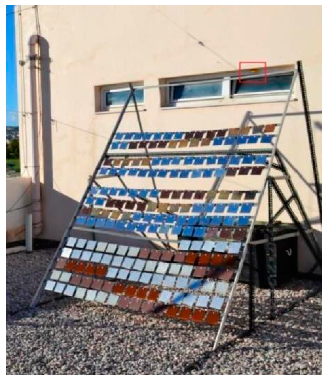
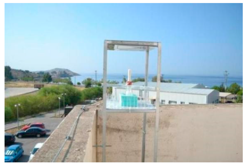
2. Materials and Methods

Aluminum, zinc, copper and unalloyed carbon steel specimens have been exposed in outdoor atmospheric conditions, on the roof of a maintenance hangar, at a distance of approximately 0.2 km from the seashore at the LGMG for a 4-year exposure period. Exposure started in 2014 at two different periods of the year, in summer and in winter, in order to determine the seasonal effects on the initial corrosion stage and eventually the long-term effects on the metal surface, as well as the evolved corrosion rates. The standard specimens of commercially pure Al (>99.5% minimum), unalloyed carbon steel, Zn (>95% minimum) and Cu (>94% minimum) were flat coupons with dimensions 100 × 100 × 1 mm³, as described in ISO 9226 [9].

Table 1. Average chemical composition (wt.%) of unalloyed carbon steel specimens.

Fe	C	Mn	S	P	Si	Ni	Cr	Cu	Al	Sn	Mo	Co	As	Nb	N	O	Other
99.44	0.07	0.32	0.03	0.007	0.007	0.02	0.02	0.04	0.01	0.004	0.003	0.003	0.0017	0.001	0.004	0.016	0.002

shows the detailed composition of the tested carbon steel samples as analyzed by an ARL3460 automatic Optical Emission Spectrometer (OES) at Halyvourgiki Inc. laboratories.

The LGMG (37 58 52.01” Ν, 023 21 55.52” Ε) [44] was selected as the exposure site due to (i) the observation of macroscopic corrosion in aircraft subassemblies and of the construction materials in helicopters, after technical inspection, and (ii) the proximity of the rural test site to the seacoast and to the surrounding industrial area of Elefsina.

Four test pieces were used for each metal and period of exposure on a rack at 45° to the horizontal facing south, as seen in Figure 1 and Figure 2. The metal structures were designed with the use of “3D CAD Design Software SOLIDWORKS’’, according to standard ISO 9225 [8] and constructed in the Laboratory of the Manufacturing Technology of NTUA. Three specimens, for each metal and period of exposure, were weighted before and after the exposure in order to measure the weight loss. The preparation, cleaning of the metal coupons (and the mass loss of the exposed metal samples) was determined after sequential pickling as per ISO 8407 [32] and the ASTM norm, G1-90 [33]. Chemical cleaning procedures for the removal of the corrosion products are described in

Table 2. Chemical cleaning procedures for removal of corrosion products after the exposure.

Metal	Chemical Bath	Time	Temperature
Aluminum	50 mL H3PO4, 30 g CrO3, distilled water to make up 1 L.	10 min	80 °C to boiling
Steel	250 mL HCl with inhibitor, distilled water to make up 1 L.	10 min	20–25 °C
Zinc	150 mL NH4OH, distilled water to make up 1 L.	5 min	20–25 °C
Copper	500 mL HCl, distilled water to make up 1 L.	3 min	20–25 °C

.

The fourth test specimen for each metal was employed for the surface analysis of the corrosion products formed. Test work was carried over 4 years, with samples taken for analysis after 3, 6, 12, 24 and 48 months during the two periods of exposure. “TableCurve 2D v5.01.01” and “Microsoft Excel” software were used for the determination of the power equations and for plotting the data relative to the corrosion loss. Corrosion rates of the tested metals were determined from the weight loss of specimens in accordance to ISO 9226 [9].

The corrosion products formed on the metal surfaces have been characterized by: (i) A FEI Quanta 200 Scanning Electron Microscope/Energy Dispersive Spectrometer (SEM/EDS, Thermo Fisher Scientific, Waltham, MA, USA) coupled with Energy Dispersive X-Ray Analysis (EDAX). The SEM images were analyzed by means of the computer program EDGE.EXE [45]. (ii) A Siemens D-500 X-ray diffractometer (with a graphite crystal monochromator and a Cu anticathode, (Siemens, Munich, Germany) based on an automatic adjustment and analysis system, with Diffract-EVA quality analysis software [46]. (iii) A Leica DMR Optical Microscope (OM, Leica Microsystems, Wetzlar, Germany). (iv) For the Al surface morphology examination, an Atomic Force Microscope Scanner (AFM, Semilab Germany GmbH, Braunschweig, Germany) DUALSCOPE 95-50 of DME was employed. (v) Examination of the presence of amorphous corrosion products on steel coupons’ surface was performed by Fourier Transform Infrared Spectrometer FT-IR4200 of Jasco (Jasco, Cremella, Italy).

A temperature (T °C) and relative humidity (RH%) data logger «Tinytag» PLUS2 (TGP-4500) was used in order to obtain the parameters of air temperature and of relative humidity, for a year, at the exact field site, as seen in the frame of Figure 1. T and RH data obtained by the data logger are also used for calculating the Time of Wetness (TOW). Τhe TOW is calculated as the length of time when the relative humidity is greater than 80% at a temperature greater than 0 °C [6]. In order to determine the airborne salinity, the chloride measurements were conducted by the Wet Candle Method for the airport according to ISO 9225 [8] and ASTM G140-02 [31] Standards. Sampling was performed every 30 days, while a new sample was positioned for further exposure. The amount of chlorides, in every sample, was measured by both the Mohr and Volhard titration methods, as well as by AgNO₃ test. Chloride measurements of the atmosphere were not feasible; however, an approximate environmental calibration based on corrosion rates’ determination and corrosion products’ characterization and literature is attempted.

In addition, three specimens of the commercially pure Al (>99.5% minimum) and the unalloyed carbon steel are also exposed for a one-year period, for two initial times of exposure. After one year, the first set of the exposed specimens was removed and another set was exposed. This process was repeated from 2014 to 2019, according to ISO and ASTM standards. A classification of the atmospheric aggressivity based on the environmental data and the corrosion rate measurements of steel and Al was conducted. The obtained gravimetric data were also used in order to examine the reliability of the CDA, and the Europe and Asia Corrosion Map at the LGMG environment.

3. Results

3.1. Regional Environmental Parameters

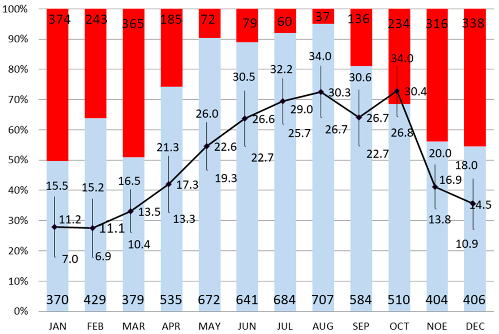
3.1.1. Pollutants

The mean annual concentration of the O₃ over the Attica region, during the period 2000-09, is almost constant at approximately 55 μg/m³ [47,48]. In a distance of 20 km from the LGMG area, where the country’s industrial core is located in the area of Elefsina, the annual mean concentration of SO₂ is at approximately 7 μg/m³ [47,49,50]. In the LGMG area, there has never been made any pollutant concentration measurements. Regarding the concentration of sulfur dioxide at the LGMG, the annual maximum concentration of the pollutant is estimated at [SO₂]_max = 2 μg/m³, according to the European Monitoring and Evaluation Program (EMEP) and several sources [47,49,50,51,52,53,54,55,56].

3.1.2. Meteorological Data

The meteorological data at LGMG area are presented in

Table 3. Meteorological data at Megara area, in brief [47,57,58,59].

Wettest Month (with Highest Rainfall)	Driest Months (with Lowest Rainfall)	Mean Annual Rainfall (Period 1958–1997)	Monthly Prevailing Wind (Period 1975–1991)	Calm	Mean Annual Wind Speed (Period 2009–2011)
December	July and August	37.29 cm	NORTHWEST (ΝW)	31%	11.22 km/h (3.17 m/s)

.

The monthly variation of the temperature-humidity data and the time of wetness are presented in Figure 3.

The time of wetness expressed in hours per year has been estimated to 2439 h/year, as reported in a previous work [60]. The RH-TOW factor is expected to affect the atmospheric corrosion of metals in a major degree. The influence of temperature on the atmospheric corrosion of many metals has a maximum at about 9–11 °C. The mean annual temperature at the airport has been 20.9 °C, as previously reported [60]. Due to the NW prevailing wind at Megara area, from inland to the seashore, and the mean annual wind speed, the salinity is expected to affect the corrosion of metals to a lesser degree than what is generally expected for a coastal site [47].

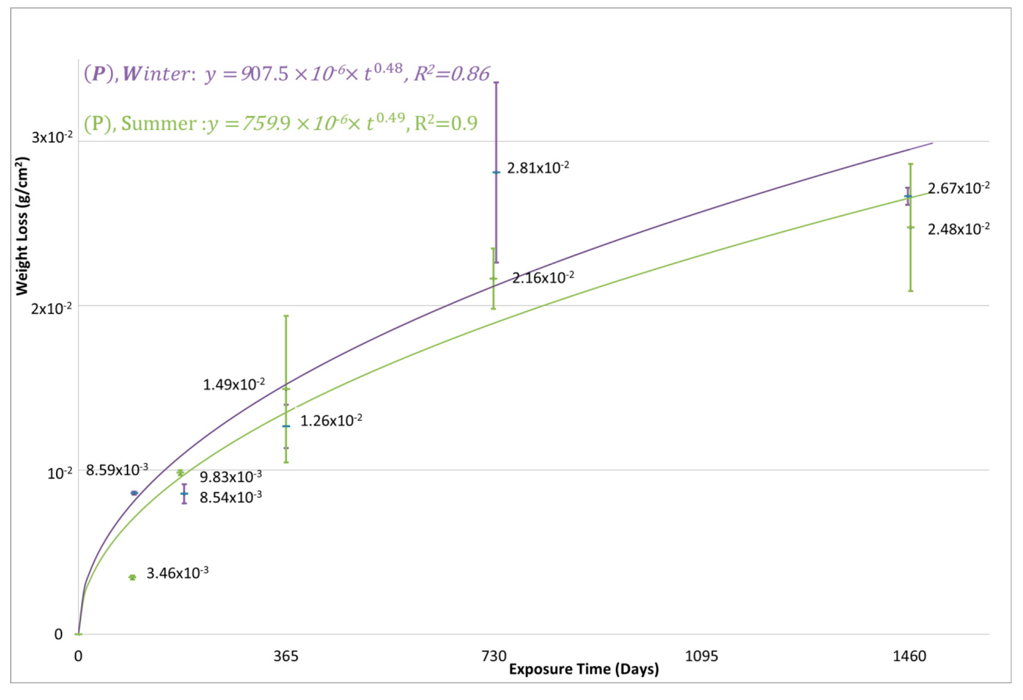
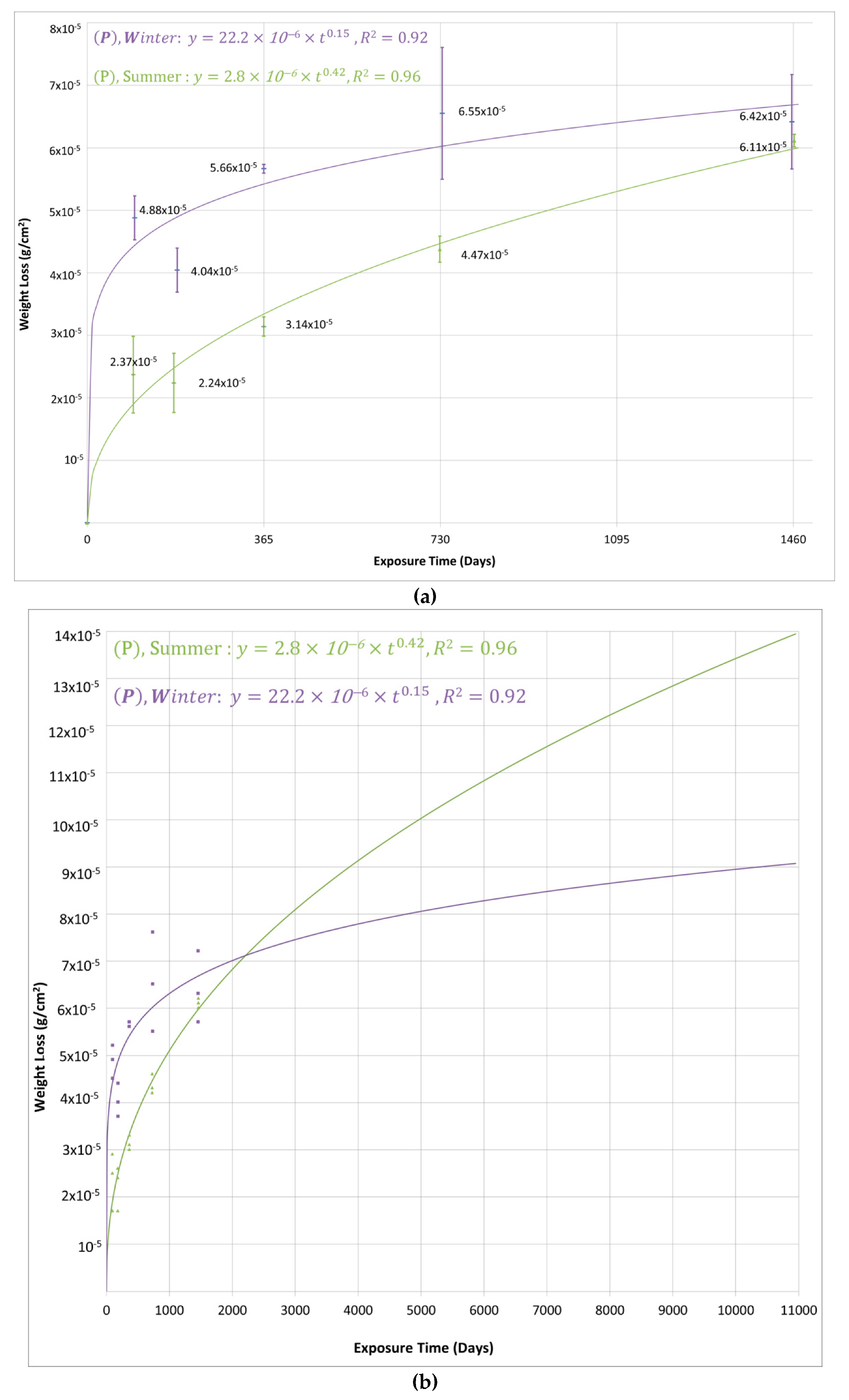
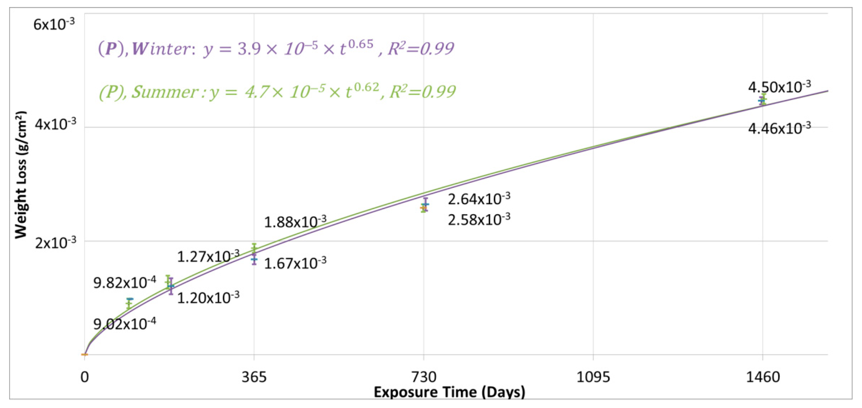
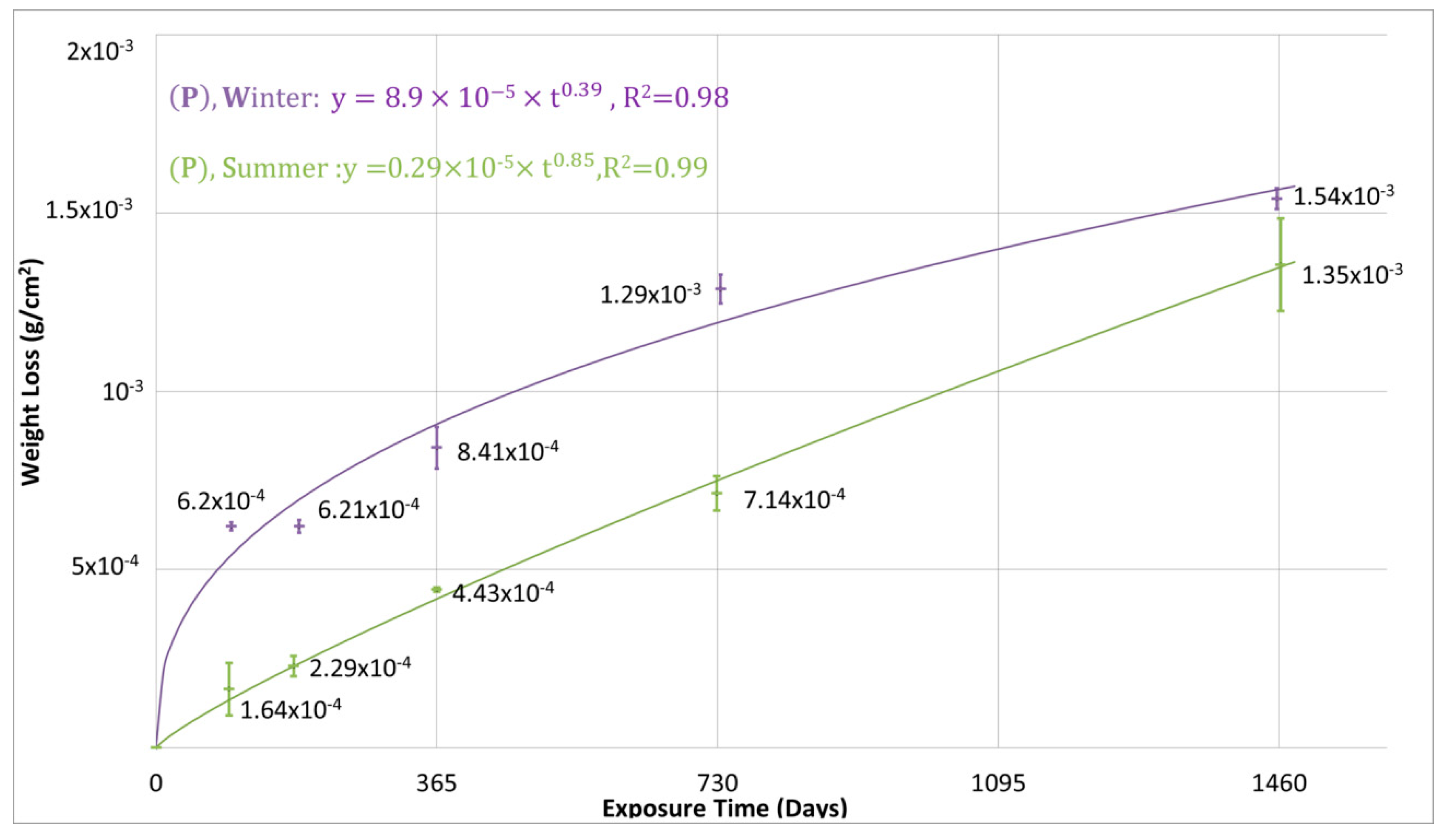
3.2. The 4-Year Corrosion Assessment of the Tested Metals and the Anticipated 30-Year Corrosion Loss

For modeling the corrosion loss with exposure time, the (power) kinetic Equation (1) was employed in the form:

$$\mathrm{y}=\mathrm{a}\times {\mathrm{t}}^{\mathrm{b}}$$

(1)

where a: constant, t: time of exposure in days and b: time exponent. The validity of the equation and its reliability to predict long-term corrosion has been demonstrated by many authors [16,23,61,62,63,64,65,66,67]. Both “a” and “b” are dependent on the climatic parameters and on the type of the metal. The constant “a” represents the corrosion loss during the first year, while the time exponent “b” represents the multi-year loss yield [68]. The higher the time exponent “b” term is the less protective is the corrosion product layer on the metal surface [69]. The statistical coefficient of determination, R², is a measure of the goodness of fit of the experimental data [69].

The representation of the corrosion data versus time and the 30-year anticipated corrosion evolution are depicted in

Table 4. Mass loss data for 1, 2 and 4 years, experimentally determined, the model kinetic parameters and the estimation of 30-year corrosion by the projection of the model equations.

Metal	Exposure Start	Average Mass Loss (g/m2)				Calculated Kinetic Equations Constants
		1 Year	2 Years	4 Years	30 Years	a	b	R2
Carbon Steel	Summer	149.1	216.4	248	709.4	759.9 × 10−6	0.49	0.9
	Winter	126.5	281	267	772.7	907.5 × 10−6	0.48	0.86
Al	Summer	0.31	0.44	0.61	1.39	2.80 × 10−6	0.42	0.96
	Winter	0.57	0.65	0.64	0.91	22.2 × 10−6	0.16	0.92
Cu	Summer	18.9	25.8	45.0	153.3	4.7 × 10−5	0.62	0.99
	Winter	16.7	26.4	44.6	161.1	3.9 × 10−5	0.65	0.99
Zn	Summer	4.4	7.1	13.5	74	0.29 × 10−5	0.85	0.99
	Winter	8.4	12.9	15.4	34.6	8.9 × 10−5	0.39	0.98

and in the power plots and Figure 4, Figure 5, Figure 6 and Figure 7 for each one of the tested metals. Table 4 shows the mass loss data for 1, 2 and 4 years, determined experimentally and the model equation parameters and the estimation of 30-year corrosion by the projection of the model equations.

Table 5. Corrosion rate of Cu, expressed in μm/year, after 1, 2 and 4 years of outdoor exposure.

Metal	Exposure Start	Corrosion Rate (μm/year)
Cu	Summer	1	1.43	1.23
	Winter	1.86	1.47	1.24

shows the corrosion rate of Cu for 1, 2 and 4 years, determined experimentally, expressed in μm/year, given by the Equation:

r_corr = Δm/(A ρ t)

(2)

where Δm is the mass loss of Cu in g, A is the surface area in m², t is the exposure time in years and ρ is the density of Cu ρ_cu = 8.96 g/cm³ [9]. Figure 4, Figure 5, Figure 6 and Figure 7 show the experimental gravimetric curves and the fitted model equations obtained for the four metals tested.

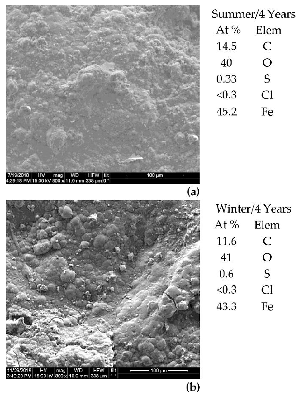
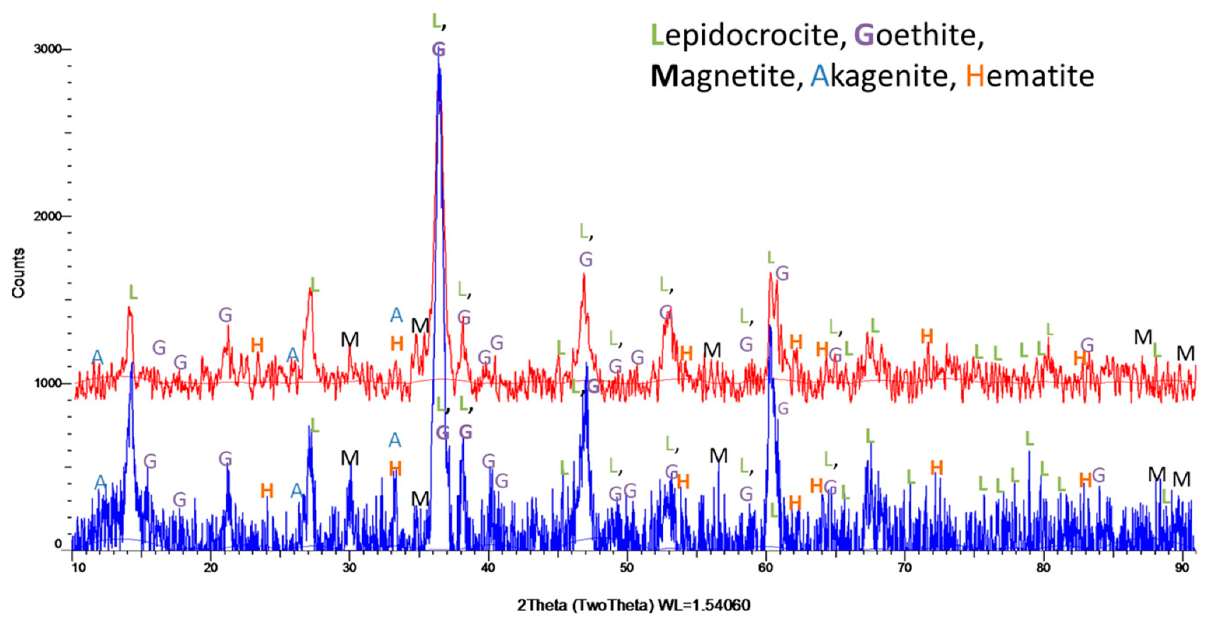
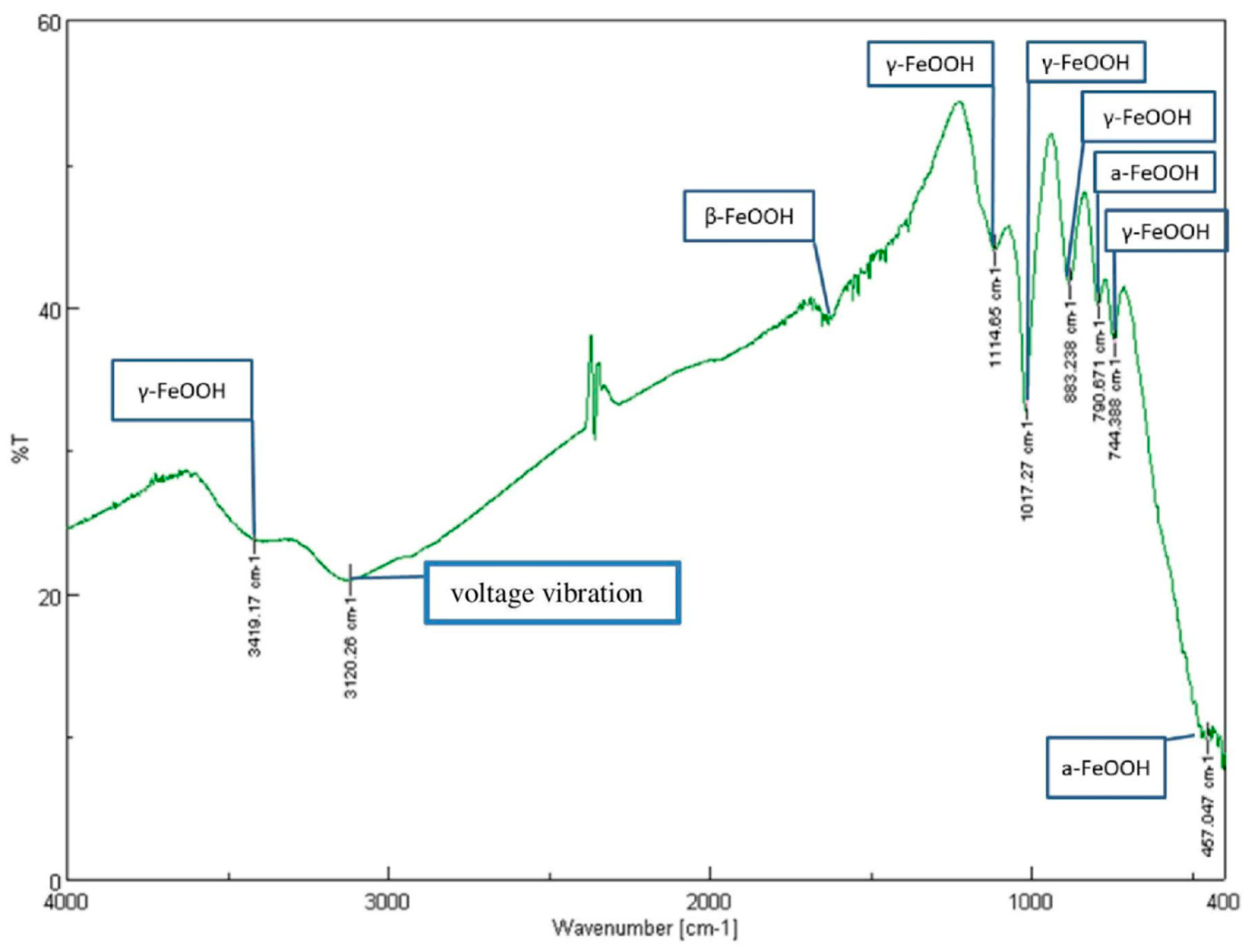
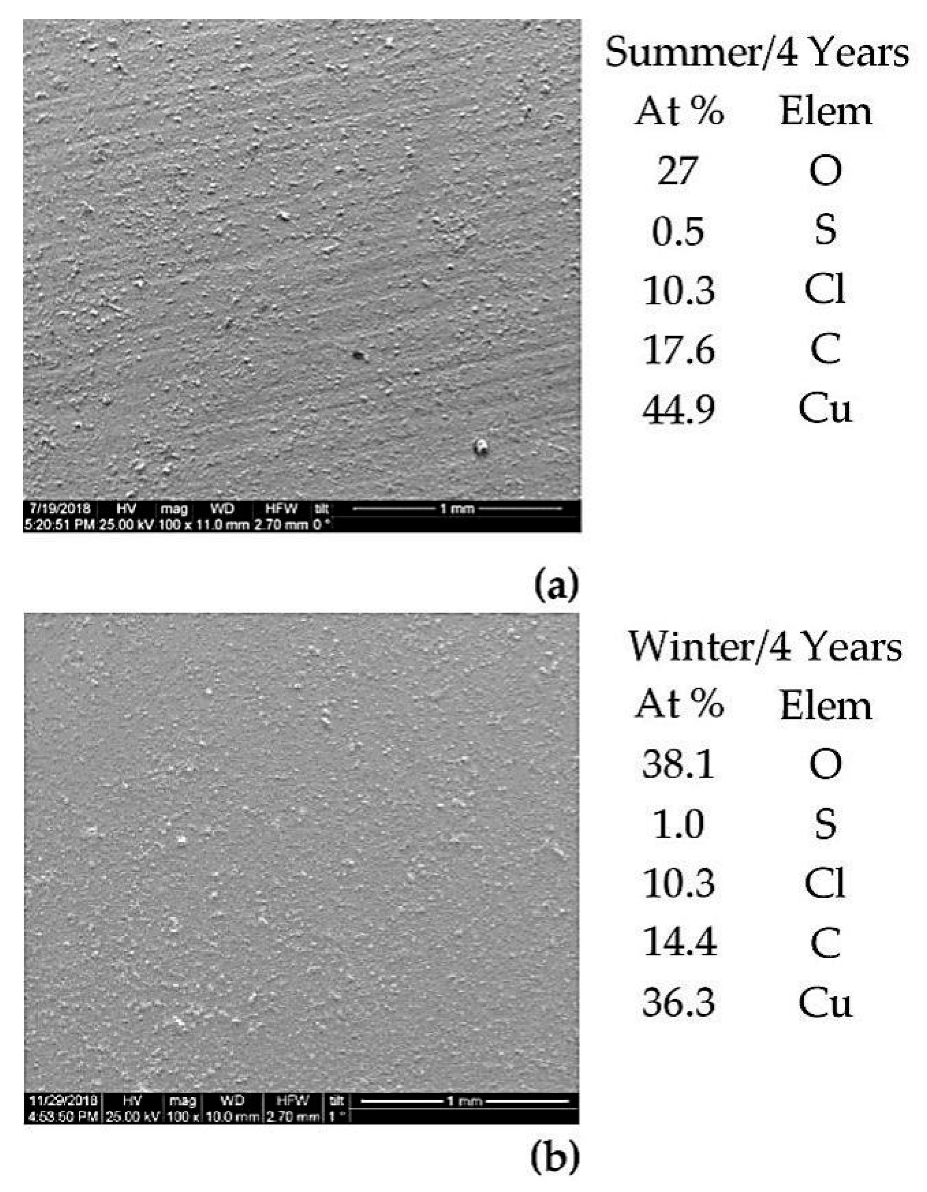
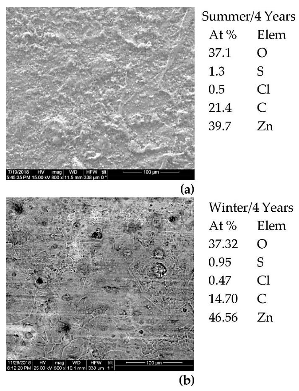
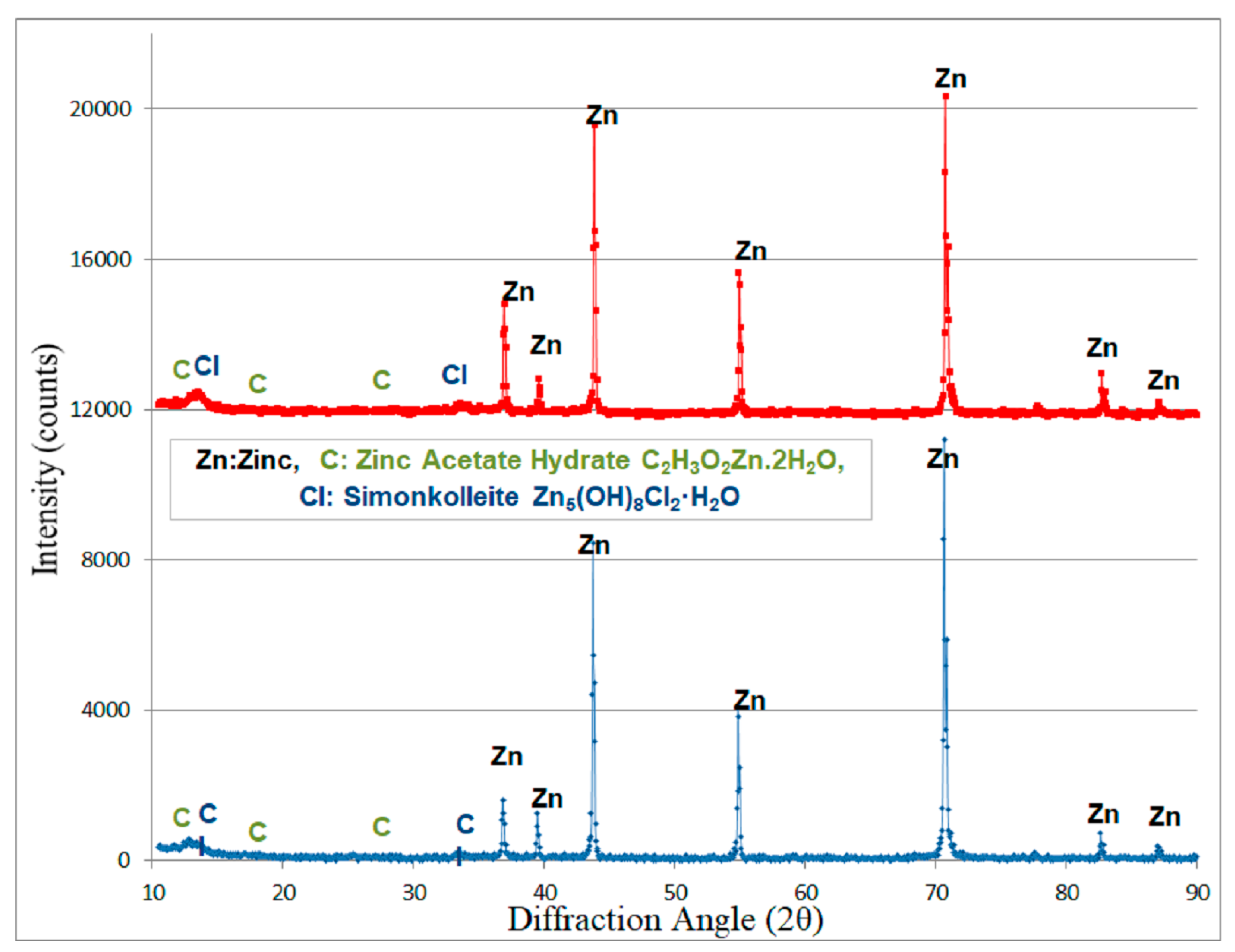
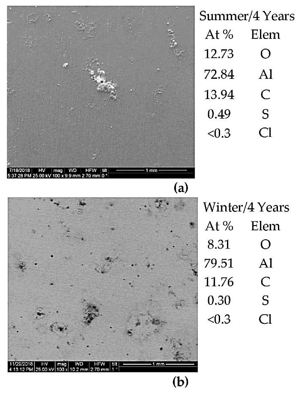
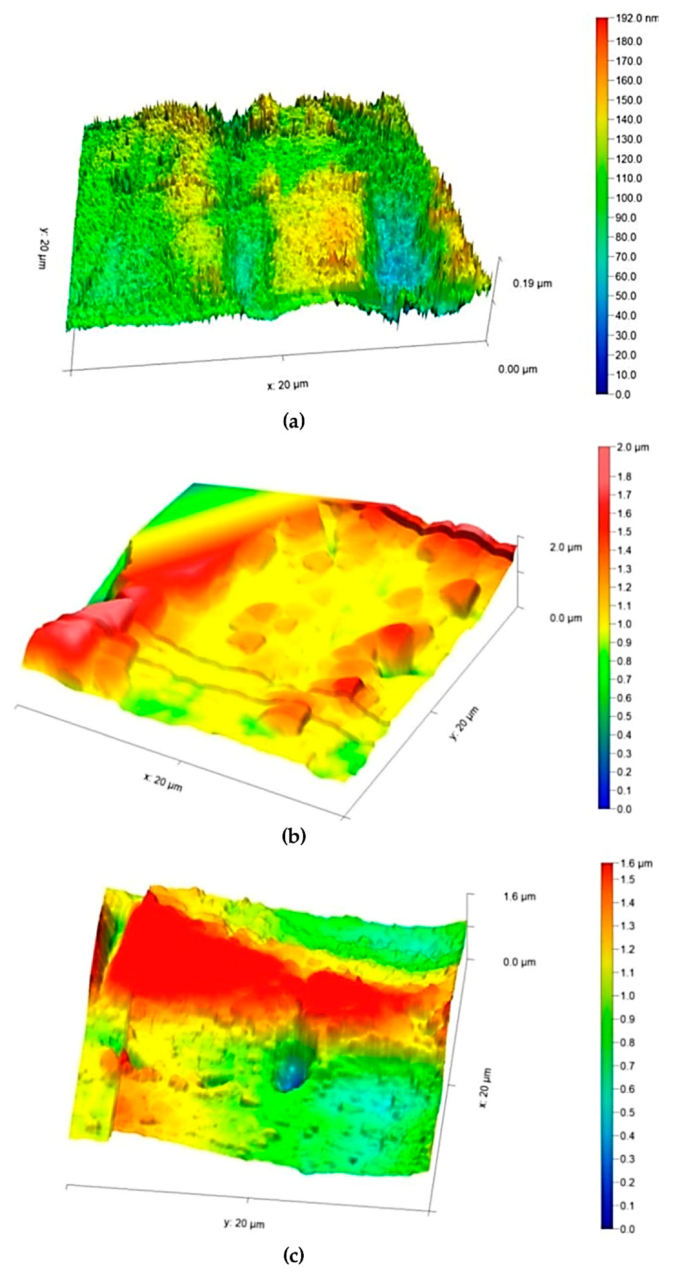
3.3. Characterization of the Metals’ Surfaces After Four Years of Exposure

It is observed that, in an area with low values of pollutants’ concentration, the corrosion attack on the downward side of the metal specimens is significantly lower than on the upward side [70]. This is also observed, both macroscopically and microscopically, in the metal specimens tested. That observation confirms (i) the low concentration of pollutants in the LGMG, especially of SO₂, and (ii) reveals the significant role of rainfall in the corrosivity of its atmosphere.

The corrosion products’ development on the steel surface observed by OM, after four years of exposure, for both initial time of exposure, is presented in Figure 8.

C, S and traces of chlorides, attributed to aircraft fuel emissions, the emissions of the vehicles traveling on the nearby motorway (0.9 km) and the proximity to the sea (0.2 km) are detected from the carbon steel specimens’ surface analysis by SEM/EDS. Carbon steel exhibits the highest concentration of O among the tested metals due to the oxides and hydroxides formed on both sides. The surface analysis by SEM/EDS on steel, after four years of exposure, is presented in Figure 9.

Growth of oxides and hydroxides is observed, both on skyward and downward sides, already from the 1st semester of the exposure, by X-ray diffraction (XRD). Lepidocrocite [γ-FeO(OH)] and traces of goethite [α-FeO(OH)] are identified after two years of exposure of carbon steel specimens’ surface in the atmosphere, independent from the initial time of exposure (summer or winter) and the side of the specimens (skyward or downward). Magnetite (Fe₃O₄) is identified on the coupons’ skyward surface, exposed during winter, after two years of exposure [46]. After four years, lepidocrocite [γ-FeO(OH)], goethite [α-FeO(OH)], magnetite (Fe₃O₄), akagenaite (β-FeOOH) and traces of hematite (Fe₂O₃) are identified on both sides of the steel specimens for both initial times of exposure. No amorphous corrosion products on steel surface were detected after examination of carbon steel specimens by XRD (Figure 10) and FTIR (Figure 11) and also mentioned by other studies [71,72,73,74,75,76,77,78,79]. The corrosion products identified by XRD and FTIR, after four years of exposure, are presented in Figure 10 and Figure 11.

In the case of the Cu specimens tested, both macroscopically and microscopically, cuprite (Cu₂O) prevalence as the main corrosion product is found. The corrosion products on Cu by OM after four years of exposure, are shown in Figure 12.

In the case of Cu, increased concentrations of O and Cl⁻ are detected by SEM/EDS. Cu exhibits the highest concentration of chlorides among the tested metals and the second higher concentration of C. On the skyward side of Cu specimens (×100), after four years of exposure, the % atomic concentration of chloride is 10.3%, independent of the initial time of exposure. The surface analysis by SEM/EDS on Cu surface, after four years of exposure, is presented in Figure 13.

Growth of Cu₂O on both the upper and lower sides of the Cu specimens has been observed since the first semester of exposure. Cu₂O is identified as the only corrosion product during the first two years of exposure by XRD. After four years of exposure, on both sides of the specimens (i) Cu₂O is identified as the main corrosion product, (ii) atacamite [Cu₂Cl(OH)₃] is also identified, as a result of the salinity on the specimens’ surface. The corrosion products identified by XRD, after four years of exposure, for both initial times of exposure, are presented in Figure 14.

In the case of Zn, no significant corrosion impact is microscopically observed during the four years of exposure. The low S concentration detected in Zn specimens by EDS, with the simultaneous absence of an S-containing corrosive product by XRD, proves a low SO₂ concentration in the LGMG area. Zn surface also measures the highest concentration of C among the tested metals, caused by aircraft fuel emissions, and the second higher concentration of oxygen, after carbon steel specimens, probably due to the synthesis of the corrosion products detected on its surface, after four years of exposure.

Chlorides are detected on the specimens’ surface, after four years of exposure, due to the proximity to the seacoast. The relative high TOW favors the dissolution of Zn chlorides in the moisture film.

After four years of exposure, zinc acetate hydrate (C₂H₃O₂Zn·2H₂O) and simonkolleite [Zn₅(OH)₈Cl₂·H₂O] are identified by XRD, as a result of the effect of aircraft fuel emissions and the proximity to the seacoast, respectively. The surface analysis by SEM/EDS and the corrosion products identified by XRD, on the Zn surface, after four years of exposure, for both initial time of exposure, are presented in Figure 15 and Figure 16.

In the case of Al, no significant corrosion impact is observed by OM, even after four years of exposure. O, S, C and traces of chlorides are detected by SEM (Figure 17), after a 4-year exposure period, despite the background pollution, the proximity to the sea, and the Al susceptibility to pitting corrosion.

No products, at both sides of the specimens, are identified by X-ray diffraction analysis on the Al surface, probably due to the small thickness of the corrosion layers.

By AFM, the mean roughness S_a (arithmetical mean height) of the 400 μm² projected areas of the skyward side of the Al 1050, before the exposure, after two and four years of exposure during summer and winter, is presented in

Table 6. The mean roughness Sa of the 400 μm² projected areas of the skyward side of the Al 1050.

Exposure Start/Time of Exposure in Years	Summer	Winter
Before the Exposure	65.2 nm
2 Years	131 nm	136 nm
4 Years	189.1 nm	214 nm

.

After two years of exposure: (i) the S_a doubles and the rolling lines appear to be filled with corrosion products and (ii) no seasonal deviations are observed regarding the roughness evolution of the Al surface. After four years of exposure, the S_a and the highest pitting depth S_v of the 400 μm² projected areas (1.157 μm during summer and 1.035 μm during winter) reveal a higher impact on the surface of the specimens exposed during summer, mainly due to the effect of higher concentration of chlorides and particulate matters (PM). The surface morphology development of the skyward side of Al 1050 by AFM, after four years of exposure is presented in Figure 18.

Pitting is detected on Al specimen’s surface, but in a much smaller extent than theoretically expected and only after two years of exposure, due to (i) the pollution of the area (low concentration of SO₂ and chloride deposition rate at the range of 0–20 mg/m²d, as described in a following paragraph); (ii) the existing particulate matters in the area, augmented seasonally by the North African dust; (iii) the meteorology of the area during summer (low RH-TOW, absence of precipitation, high temperatures and low wind speed or calm) and (iv) the presence of the aircraft in the area. During the transition spring and autumn periods, the impact of African dust reaches its peak and increases the particulate matters’ concentrations in the Greek region [80]. The mean monthly concentration of PM, during the transition spring and autumn periods, is 25–40 μg/m³ [80]. The continuous take-offs/landings and technical tests, during summer (driest months), provoke the maximization of the concentration of the pollutants locally, the continuous resuspension and dry re-deposition of the contaminated by the pollutants and by chlorides’ (due to the proximity to the sea) particulate matters, on their peak concentration. These effects lead to a relatively higher pitting, in density and depth, of the Al exposed, starting in summer, in relation to the Al exposed, starting in winter, as it is presented in

Table 7. Maximum depth of pits observed on the surface of Al and evaluation of pitting corrosion by OM in accordance with ISO 8993:1989.

Exposure Start	2 Years of Exposure		4 Years of Exposure
	Maximum Pitting Depth in μm	Rating	Maximum Pitting Depth in μm	Rating
Summer	2	C4	2	D5
Winter	1.0	B5	1.0	D2

. The rating system for the evaluation of pitting corrosion on Al was performed in accordance with ISO 8993 [81], after 2 and four years of exposure. The ISO rating has been conducted visually and the estimation of the average pitting depth in μm by OM.

Due to the combustion of fossil fuels at the airport region, an atomic concentration of at least 11.5% of C is detected to all metal specimens’ surfaces by SEM, after the first two years of exposure.

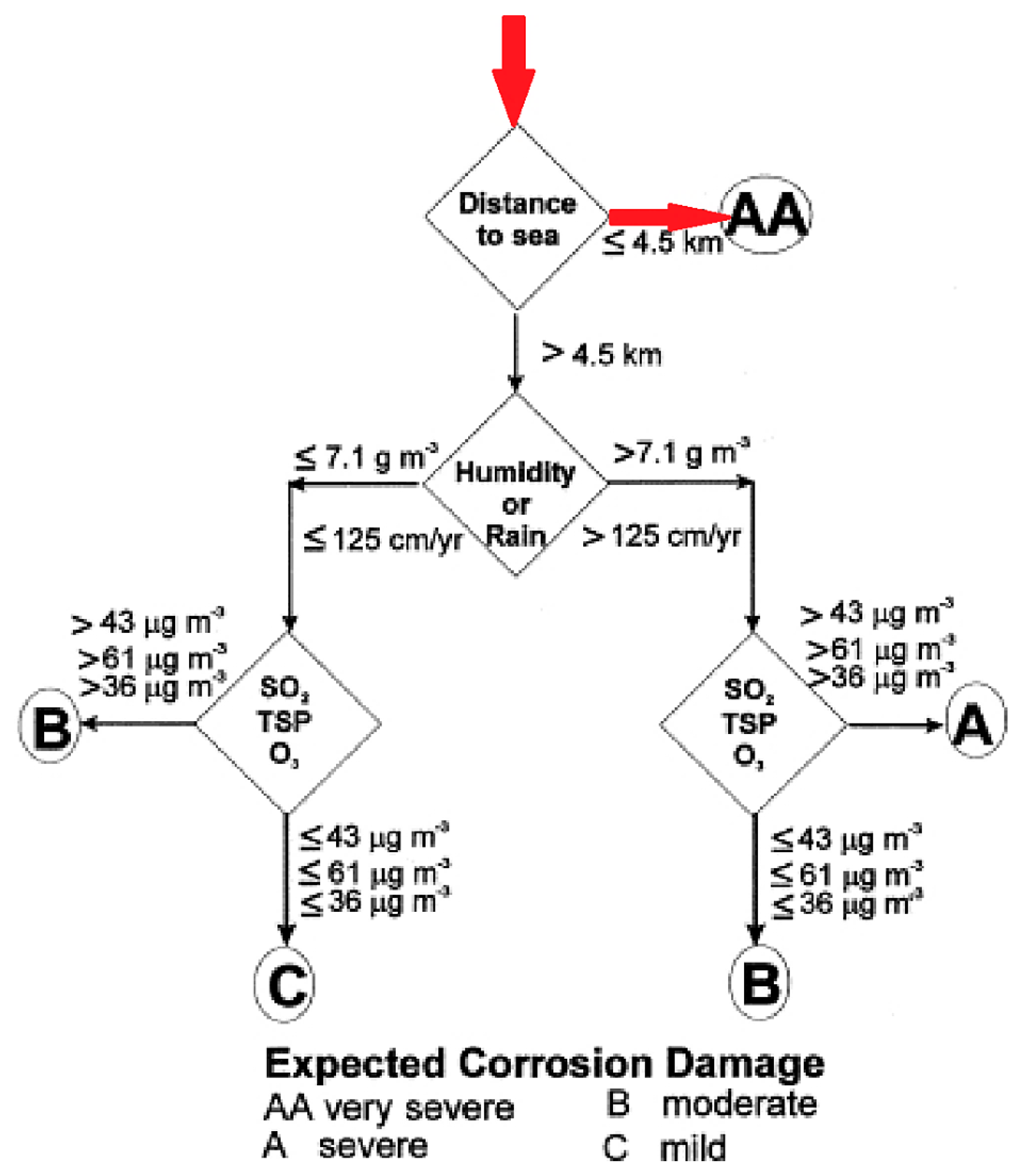
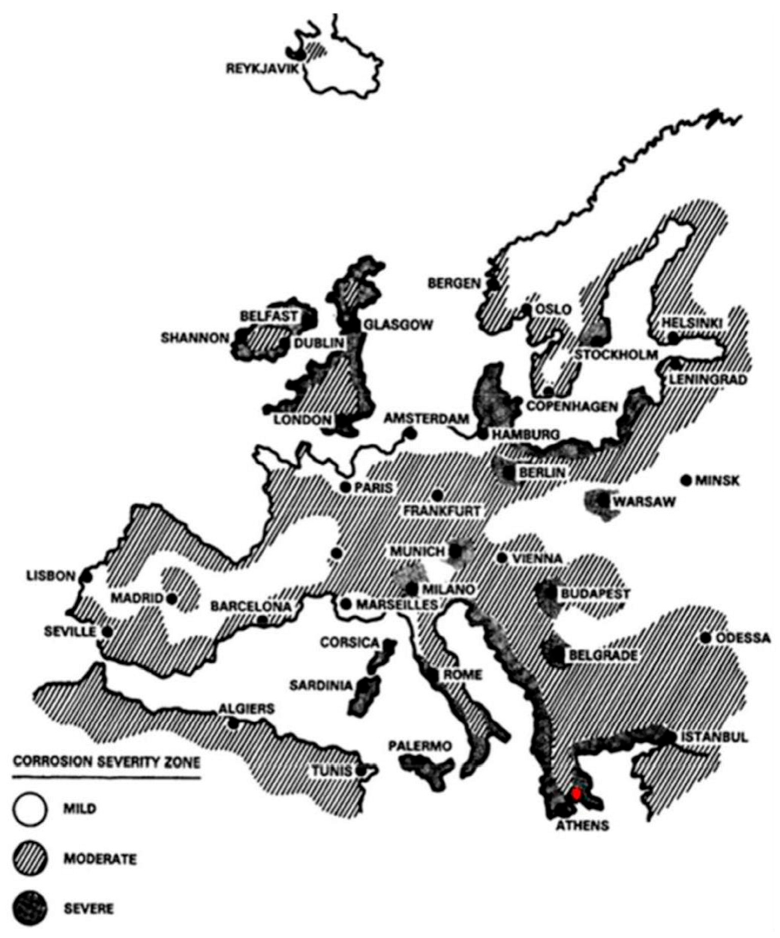
3.4. Classification of the Corrosivity of the Pachi Airport Atmosphere

With a view to the development and the specification of optimized corrosion evolution and protection for manufactured products, data on the corrosivity of the atmosphere are considered essential. The corrosivity category is a technical characteristic which provides a basis for the selection of materials and, consequently, protective measures in atmospheric environments subject to the demands of the specific application, particularly with regard to service life [9].

The airport atmosphere is classified by S-containing substances represented by SO₂, in accordance with ISO 9223 [6], in pollution category P₀ ([SO₂] < 12 μg/m³), which is accounted to be background pollution by SO₂ and insignificant from the view point of corrosion. The TOW is estimated in 2439 h/year. As a result, the atmosphere is classified of TOW as «T3», according to ISO 9223:1992 [6].

Considering the (i) the corrosion rate of Cu, (ii) the development of corrosion products on the tested metals’ surface, (iii) the pitting corrosion of Al and (iv) the atomic Cl concentration on the tested metals’ surface, during the first four years of exposure, it is estimated that the salinity deposition rate at the LGMG does not exceed the threshold of 20 mg/(m²d), which is the threshold deposition rate that would result in significant material deterioration [82]. Thus, the deposition rate of chlorides expected at the range of 0–20 mg/(m²d), seems to be better related to the observed corrosive environment. Therefore, the atmosphere of the airport, in relation to airborne salinity pollution, is rated as pollution category S₀, chloride deposition rate lower than 3 mg/(m²d), or as pollution category S₁, chloride deposition rate in mg/(m²d): 3 < S < 60, in accordance with the standard ISO 9223 [6].

The characterization of an outdoor test site with respect to its corrosivity can be accomplished by determining the corrosion rate of standard specimens exposed for one year to the atmosphere at the respective location (direct corrosivity evaluation). The average chemical composition of Al (>99.5% minimum) and carbon steel (Table 1) specimens used at this study meet the requirements described by ISO 9226 [9]. The corrosion rate of carbon steel and Al for the first year of exposure for the five different corrosion categories, according to ISO9223, is presented in

Table 8. Corrosion rates for the first year of exposure for the different corrosion categories according to ISO 9223 [6].

Corrosion Category	Carbon Steel (g/m2year)	Aluminum (g/m2year)
C1	≤10	Negligible
C2	11–200	≤0.6
C3	201–400	0.6–2
C4	401–650	2–5
C5	651–1500	5–10

.

The classification of the atmospheric corrosivity, for carbon steel and Al is presented in

Table 9. First year of exposure corrosion rate of carbon steel and Al and ISO classification of the atmosphere aggressivity at the LGMG according to ISO:9223 [6], after repeated experiments of a one-year period of outdoor exposure from 2014 to 2019.

Metal (g/m2):	Carbon Steel			Aluminum
/Period of Initial Exposure	Mean Value	Standard Deviation	Max. Value	Mean Value	Standard Deviation	Max. Value
Summer	148.1	25.7	195.2	0.308	0.016	0.331
Winter	123.5	15.6	140.7	0.562	0.007	0.571
ISO Classification of the LGMG Atmosphere	C2 «LOW»			C2 «LOW»

.

The higher first-year corrosion rate of carbon steel specimens, exposed during summer, is primarily caused by the background pollution of the area and the high conductivity of the steel specimens’ surface due to the existing PM in the area enriched by the North African dust (PM) during the initial time of exposure. The higher corrosion rate for the first-year of Al, exposed during winter, can be attributed to an easier Al³⁺ diffusion through the formed oxide with the humidity presence. The critical parameters taken into consideration in order to evaluate the atmosphere aggressivity, according to the CDA, are presented in

Table 10. Critical parameters taken into consideration in order to evaluate the atmosphere aggressivity, according to the CDA, in relation to the limits set by the algorithm.

Critical Parameters/Airport	Distance to Sea/CDA Limit	Total Annual Rainfall/CDA Limit	Ozone (O3) Concentration/CDA Limit
Pachi	0.2km < 4km	37.29 < 125 cm/year	55 > 36 μg/m3

.

4. Discussion

4.1. Corrosion Patterns Related to Each Metal Type

The main findings assessed by the 4-year atmospheric corrosion experiments at the LGMG can be summarized as follows:

In the case of carbon steel, the high RH-TOW during the period December-March, the decisive influence of the rainfall during winter and of temperature, during January and February, increase the corrosion of steel. Multi-year corrosion evolution shows that the sea chlorides, from natural airborne salinity, have an accelerating effect on the corrosion rate of steel, that is also observed by other researchers [83,84]. Taking into account the zero influence of sulfur-containing substances on atmospheric corrosion of the tested metals at the LGMG microclimate, the low corrosion rate of steel specimens also indicates a relatively low chloride deposition rate. The O₃ pollutant has little effect in steel corrosion rate [85]. Unalloyed carbon steel showed increased corrosion among the tested metals.

During the 30-year corrosion projection, the factors which led to a relatively high corrosion rate of the steel samples are:

(i)

The high relative humidity, the atmospheric precipitation (rain) and the temperature play the primary role.

(ii)

Salinity and particulate matters play a secondary role to the corrosion rate.

(iii)

Finally, the synergy of the above factors with the air pollutants (aircraft emissions, etc.).

In the case of Al, S compounds and salinity affect the “a” value much less than the other three metals [68]. Al exhibits the lowest “a” value than the other tested metals (Table 4). Al also exhibits the lowest time exponent “b” values than the other metals tested, which verifies the corrosion protectiveness of the corrosion product layer of Al₂O₃ on the metal surface. The “b” values are not strongly affected by environmental variations, due to the Al₂O₃ spontaneous formation upon exposure in the environment, which protects the metal substrate. However, despite the low exponent values observed, the “b” shows higher values in the specimens starting exposure in the summer than those in winter, which shows the following:

(i)

In the summer months, under the influence of airborne salinity and particulate matters, the corrosion product layer on Al surface is less protective than its counterpart in the winter months, where higher TOW and rainfall prevail.

(ii)

Airborne salinity and PM are anticipated to play the dominant role in the corrosion of aluminum in these atmospheres (Figure 5b).

During the four first years of exposure, relative high RH-TOW and rainfall, during the period December-March, and the mean monthly temperature, during January and February, also guide to the relatively higher corrosion attack. During the 4-year corrosion, evolution is observed that the corrosion values of Al specimens is less than 0.30 g/m²a, mainly due to the metal attack by the chemical solution used during chemical removal of the alumina film during cleaning in order to calculate the gravimetric weight loss rather than by the aggressivity of the atmosphere [84]. After 5.5 years of exposure, the corrosion rate of the Al specimens, exposed during summer, is anticipated to be higher than those exposed during winter, mainly due to the impact of salinity, because of the proximity to the sea, and the effect of the particulate matters, as it is also observed by other researchers [83]. Al corrosion rate is the lowest among the tested metals, two orders of magnitude lower than that of steel.

During the 30-year corrosion evolution, the factors which lead to a relatively high corrosion rate of the Al surfaces are:

(i)

Chlorides and PM are anticipated to be the most important causes of corrosion of Al alloys in the specific atmosphere.

(ii)

The high RH, the atmospheric precipitation (rain) and the temperature play a secondary role.

(iii)

Finally, the synergy of the above factors with the pollutants.

In the case of Cu, salinity and TOW strongly affect both the time exponent and the “a” values [68]. During the multi-year corrosion projection, Cu corrosion rate is an order of magnitude lower than that of steel and independent of the initial period of exposure. Cu has lower corrosion rate than steel because of its low thermodynamic tendency to react (noble potential compared to iron). Cu also exhibits the highest coefficient of determination value (R² = 0.99). The corrosion rate of Cu, which is less than 2 µm/year (Table 5) in the first four years of exposure, indicates that salinity is less than 20 mg/(m² d) Cl⁻ [83]. Μoisture, salinity, precipitation (rainfall) and O₃ are the factors playing a decisive role in corrosion of Cu in the airport area.

During the 30-year corrosion projection, the factors which led to a relatively high corrosion rate of the Cu samples are:

(i)

The high relative humidity, the atmospheric precipitation (rain) and the concentration of O₃ in the atmosphere are the dominant factors in the long-term corrosion of Cu.

(ii)

Chloride deposition rate has a secondary, but significant, role in corrosion rate.

In the case of Zn, the environmental variables do not significantly affect the protectivity of the corrosion product layer on the metal surface. In more detail, TOW and chlorides influence the time exponents to a small extent [68].

During the four years of exposure:

(i)

From the first year of exposure, Zn exhibits a corrosion rate dependent of the period initially exposed and an order of magnitude lower than steel, a fact that has been observed by other researchers [86]. Higher RH, during the initial time of exposure, plays a catalytic role in the corrosion rate of Zn [86], especially during the first four years of exposure. The synergistic effect of the relatively high moisture with SO₂ [56] and relatively high O₃ concentration [87] in the atmosphere increases its corrosion rate.

(ii)

The exponent “b” shows values far higher for the specimens exposed in the summer. The corrosion layer of the specimens exposed during the summer, under the influence of the airborne salinity, the particulate matters and the maximizing of concentration of the pollutants (mainly CO₂ and O₃) is less protective than its counterpart of the specimens exposed during the winter months, where high humidity and, especially, atmospheric precipitations (rainfall) provoke a washing out of the chlorides and pollutants from the metal surfaces.

In a marine atmosphere, the corrosion of Zn is a direct function of TOW and the chloride pollution level [88]. After 5.5 years of exposure, the anticipated corrosion evolution shows that Zn specimens exposed during summer exhibit a steadily higher corrosion rate, than those exposed during winter, in contrary with the first years of exposure. The 30-year corrosion evolution of Zn shows that the specimens initially exposed during summer are anticipated to have twice the weight of metal loss than those exposed during winter (Table 4), mainly due to the effect of:

(i)

Higher salinity deposition rate.

(ii)

Higher concentration of PM (African dust, particle resuspension and redeposition due to aircraft take-offs and landings, etc.).

(iii)

Higher concentration of pollutants, especially of CO₂, mainly from the combustion fuels of aircraft.

(iv)

Higher O₃ concentration.

(v)

The decisive effect of the rain on washing out the chlorides and the pollutants from the tested metals’ surface during winter.

4.2. Aspects of Gravimetric Data Analysis and Interpretation

The gravimetric data acquired for the exposure starting at winter showed that higher weight loss values are obtained during the first three months for Al, steel and Zn causing deviations from fitted curves. This can be attributed to the water-solubility of the initial corrosion products. From the 6-month experimental data, it is evident that both corrosion film dissolution and water-insoluble corrosion products’ accumulation takes place.

The chloride deposition rate in the LGMG is estimated on the basis of the:

(i)

The corrosivity of the atmosphere regarding carbon steel and Al classification as C2 “low”, according to ISO 9223.

(ii)

The low concentration of chlorides on the Al, Zn and steel surfaces.

(iii)

The pitting corrosion observed on Al surface, with maximum depth of 2 μm, after four years of exposure, at a distance of approximately 0.2 km from the seacoast.

(iv)

The average annual loss of Cu, less than 2 µm/year during the first four years of exposure.

Concerning the results of gravimetric analysis on carbon steel and aluminum specimens, after the first year of exposure, with initial time of exposure the 25th of May and the 25th of November of each year from 2014 to 2019:

(i)

The higher first-year corrosion rate of carbon steel specimens, exposed during summer, is primarily caused by the salinity and the background pollution of the area. The high conductivity of the steel surface by particulate matters acts as seeding for the water vapors to form water droplets. The seasonal presence of the African dust increases the effect.

(ii)

The higher first-year of aluminum, exposed during winter, can be attributed to an easier Al³⁺ diffusion through the formed oxide with the humidity presence.

4.3. Comparison of Three Different Approaches for Corrosive Environment Classification

The classification of atmospheric aggressivity and the expected corrosion damage to carbon steel and Al alloy components of the aircrafts at the Airport, according to the ISO and the CDA [18,19] methodologies and the Europe and Asia Corrosion Map [89], are presented in Figure 19 and Figure 20.

The results of the three methodologies employed for the classification of the corrosivity of the LGMG atmosphere are presented in

Table 11. Synoptic comparison of the results of the classification of the corrosivity of the LGMG atmosphere according to ISO [6,7,8,9] and CDA [18,19] methodologies, and Europe and Asia Corrosion Map [89].

Site of Exposure	Classification of the Corrosivity of LGMG Atmosphere According to:	Metal Specimens
		Carbon Steel	Aluminum
LGMG	ISO	C2 «LOW»	C2 «LOW»
	CDA	AA «very severe»
	«Europe and Asia Corrosion Map»	«SEVERE»

:

After a comparison of the results of the meteorological and pollution data, and of the gravimetric results on carbon steel and Al specimens exposed at the coastal site of Pachi to the expected corrosion damage, estimated by the CDA and the Europe and Asia Corrosion Map, it is proved that both the CDA and Europe and Asia Corrosion Map do not provide a good correlation between the predicted and the actual corrosion damage at the LGMG. On the contrary, the ISO classification methodology provides a good correlation among corrosivity of atmosphere and actual carbon steel and Al corrosion damage in the specific atmosphere.

5. Conclusions

1. LGMG atmosphere is classified, according to the ISO 9223:

TOW was characterized as T3. The area has been classified in pollution category P₀, which is considered to be background pollution by SO₂ and insignificant from the point of view of corrosion attack. The corrosivity of the atmosphere, regarding carbon steel and Al, has been classified as C2 “low”. The chloride deposition rate in the LGMG is estimated at the range of the values 0 < S < 20 mg/m²d, and the area has been classified in pollution category S₀ or S_1.

2. The 4-year experimental weight loss curves show that:

The corrosion rates at the coastal site of Pachi are ranked in order of decline: carbon steel > Cu > Zn > Al. No seasonal deviations are observed regarding the corrosion rates of Cu specimens during the exposure. Corrosion rate of Al is two orders lower than steel. The corrosion value of Al specimens is partially due to the metal attack by the chemical reagent used during chemical cleaning in order to calculate the gravimetric weight loss. Corrosion rate of Zn and Cu is an order lower than steel.

During the first four years of exposure, the specimens exposed during winter show higher corrosion rates than those exposed during summer. RH is identified as the major factor of corrosion of the tested metals. Precipitation and temperature are also recognized as main corrosion factors. Depending on the metal, these factors, in combination with: (i) Airborne salinity, PM and the high concentration of O₃ lead to a relatively high corrosion rate of Cu. (ii) Airborne salinity and CO₂ lead to a higher corrosion rate of Zn. (iii) Airborne salinity and PM lead to a higher corrosion rate of steel and Al alloy. Uniform corrosion is observed on the surface of the steel specimens and pitting corrosion is observed on the surface of the Al.

3. During the 30-year corrosion evolution:

In the case of carbon steel, the specimens exposed during winter show higher corrosion rates than those exposed during summer. The steel corrosion rate is the highest among the metals tested.

In the case of Cu, the metal specimens exposed during winter show higher corrosion rates than those exposed during summer.

In the case of Zn, the metal specimens exposed during summer are expected to show higher corrosion rates than those exposed during winter, after 5.5 years of exposure. Zinc specimens, exposed during summer, are expected to have double metal loss than those exposed during winter, after 30 years of exposure.

In the case of Al, the metal specimens exposed during summer are anticipated to show higher corrosion rates than those exposed during winter, after 5.5 years of exposure. The corrosion rate of Al is expected to remain the lowest among the tested metals and by two orders lower than steel. The corrosion curves, as well as the evolution of the maximum pitting depth, indicate the self-stopping nature of pitting corrosion of aluminum.

4. After a comparison of the results of gravimetric analysis on carbon steel and Al specimens to the expected corrosion damage estimated by the CDA and the classification of atmospheric aggressivity according to the Europe and Asia Corrosion Map, it is proved that the CDA and the Europe and Asia Corrosion Map do not provide a good correlation between the predicted and the actual corrosion damage at the LGMG, regarding carbon steel and Al. The ISO classification methodology provides a good correlation among corrosivity of atmospheres and actual carbon steel and aluminum corrosion damage in the specific atmosphere.

References

1. Simillion, H.; Dolgikh, O.; Terryn, H.; Deconinck, J. Atmospheric Corrosion Modeling. Corros. Rev. 2014, 32, 73–100. [Google Scholar] [CrossRef]
2. United States Department of Transportation, National Transportation Library. Available online: https://rosap.ntl.bts.gov/view/dot/40697 (accessed on 20 February 2020).
3. Biezma, M.V.; San Cristóbal, J.R. Methodology to Study Cost of Corrosion. Corros. Eng. Sci. Technol. 2005, 40, 344–352. [Google Scholar] [CrossRef]
4. Thompson, N.G.; Yunovich, M.; Dunmire, D. Cost of Corrosion and Corrosion Maintenance Strategies. Corros. Rev. 2007, 25. [Google Scholar] [CrossRef]
5. Xu, N.; Zhao, L.; Ding, C.; Zhang, C.; Li, R.; Zhong, Q. Laboratory Observation of Dew Formation at an Early Stage of Atmospheric Corrosion of Metals. Corros. Sci. 2002, 44, 163–170. [Google Scholar] [CrossRef]
6. International Organization for Standardization. Corrosion of Metals and Alloys: Corrosivity of Atmospheres: Classification, Determination and Estimation (ISO/DIS Standard No. 9223); International Organization for Standardization: Geneva, Switzerland, 1992. [Google Scholar]
7. International Organization for Standardization. Corrosion of Metals and Alloys: Corrosivity of Atmospheres: Guiding Values for the Corrosivity Categories (ISO/DIS Standard No. 9224); International Organization for Standardization: Geneva, Switzerland, 1992. [Google Scholar]
8. International Organization for Standardization. Corrosion of Metals and Alloys: Corrosivity of Atmospheres: Measurement of Pollution (ISO/DIS Standard No. 9225); International Organization for Standardization: Geneva, Switzerland, 1992. [Google Scholar]
9. International Organization for Standardization. Corrosion of Metals and Alloys: Corrosivity of Atmospheres: Methods of Determination of Corrosion rates of Standard Specimens for the Evaluation of Corrosivity (ISO/DIS Standard No. 9226); International Organization for Standardization: Geneva, Switzerland, 1992. [Google Scholar]
10. Morcillo, M.; Almeida, E.; Chico, B.; de la Fuente, D. Analysis of ISO Standard 9223 (Classification of Corrosivity of Atmospheres) in the Light of Information Obtained in the Ibero-American Micat Project. In Outdoor Atmospheric Corrosion; Townsend, H., Ed.; ASTM International: West Conshohocken, PA, USA, 2002; pp. 59–72. [Google Scholar] [CrossRef]
11. Kreislova, K.; Knotkova, D. Corrosion Behaviour of Structural Metals in Respect to Long-Term Changes in the Atmospheric Environment. In Proceedings of the EUROCORR 2011, Stockholm, Sweden, 5–8 September 2011. [Google Scholar]
12. Kreislova, K.; Knotkova, D. The Results of 45 Years of Atmospheric Corrosion Study in the Czech Republic. Materials 2017, 10, 394. [Google Scholar] [CrossRef] [Green Version]
13. Tidblad, J.; Kucera, V.; Ferm, M.; Kreislova, K.; Brüggerhoff, S.; Doytchinov, S.; Screpanti, A.; Grøntoft, T.; Yates, T.; de la Fuente, D.; et al. Effects of Air Pollution on Materials and Cultural Heritage: ICP Materials Celebrates 25 Years of Research. Int. J. Corros. 2012, 2012. [Google Scholar] [CrossRef]
14. Mendoza, A.; Corvo, F. Outdoor and Indoor Atmospheric Corrosion of Non-Ferrous Metals. Corros. Sci. 2000, 42, 1123–1147. [Google Scholar] [CrossRef]
15. Tidblad, J. Atmospheric Corrosion of Metals in 2010–2039 and 2070–2099. Atmos. Environ. 2012, 55, 1–6. [Google Scholar] [CrossRef]
16. Pourbaix, M. The Linear Bilogarithmic Law for Atmospheric Corrosion. In Atmospheric Corrosion; Ailor, W.H., Ed.; J. Wiley & Sons: New York, NY, USA, 1982; pp. 107–121. [Google Scholar] [CrossRef] [Green Version]
17. McCuen, R.H.; Albrecht, P.; Cheng, J.G. A New Approach To Power-Model Regression Of Corrosion Penetration Data. In Corrosion Forms and Control for Infrastructure; ASTM STP 1137; Chaker, V., Ed.; American Society for Testing and Materials: West Conshohocken, PA, USA, 1992; pp. 46–76. [Google Scholar]
18. Summitt, R.; Fink, F. PACER LIME, Part 2. Experimental Determination of Environmental Corrosion Severity; Michigan State University: East Lansing, MI, USA, 1980. [Google Scholar]
19. Research and Technology Organization. Corrosion Fatigue and Environmentally Assisted Cracking in Aging Military Vehicles; Tech. Rep. AG-AVT-140; NATO: Neuilly, France, 2011. [Google Scholar]
20. Kenny, E.D.; Esmanhoto, E.J. Tratamento Estatistico do Desempenho de Materiais Metalicos no Estado do Parana. In XVII Congresso Brasileiro de Corrosao; Anais; ABRACO, T-24: Rio de Janeiro, Brazil, 1993; pp. 297–308. [Google Scholar]
21. Kenny, E.D.; Esmanhoto, E.J. Corrosao do aco-carbono por intemperismo natural no Estado do Parana. In IV Seminario de Materiais no Setor Elιtrico; Anais; Copel/UFPR: Curitiba, Brazil, 1994; pp. 377–382. [Google Scholar]
22. Feliu, S.; Morcillo, A.; Feliu Jr., S. The Prediction of Atmospheric Corrosion from Meteorological and Pollution Parameters—I. Annual corrosion. Corros. Sci. 1993, 34, 403–414. [Google Scholar] [CrossRef]
23. Feliu, S.; Morcillo, A.; Feliu Jr., S. The Prediction of Atmospheric Corrosion from Meteorological and Pollution Parameters—II. Long-term forecasts. Corros. Sci. 1993, 34, 415–422. [Google Scholar] [CrossRef]
24. Morcillo, M.; Almeida, E.M.; Rosales, B.M. Functiones de Dano (Dosis/Respuesta) de la Corrosion Atmospherica en Iberoamerica, Corrosion y Proteccion de Metales en las Atmosferas de Iberoamerica; Programma CYTED: Madrid, Spain, 1998; pp. 629–660. [Google Scholar]
25. Cai, J.; Cottis, R.A.; Lyon, S.B. Phenomenological Modelling of Atmospheric Corrosion Using an Artificial Neural Network. Corros. Sci. 1999, 41, 2001–2030. [Google Scholar] [CrossRef]
26. Jančíková, Z.; Zimný, O.; Koštial, P. Prediction of Metal Corrosion by Neural Networks. Metalurgija 2013, 52, 379–381. [Google Scholar]
27. Cai, Y.; Zhao, Y.; Ma, X.; Zhou, K.; Chen, Y. Influence of Environmental Factors on Atmospheric Corrosion in Dynamic Environment. Corros. Sci. 2018, 137, 163–175. [Google Scholar] [CrossRef]
28. Mikhailov, A.A.; Tidblad, J.; Kucera, V. The Classification System of ISO 9223 Standard and the Dose-Response Functions Assessing the Corrosivity of Outdoor Atmospheres. Prot. Metals 2004, 40, 541–550. [Google Scholar] [CrossRef]
29. University of the Aegean. Department of Environment. Available online: http://www1.aegean.gr/lid/internet/elliniki_ekdosi/TEL_DIMOSI/Paper_Periferiakotita.pdf (accessed on 20 February 2020).
30. World.bymap.org/Coastline Lengths. Available online: http://world.bymap.org/Coastlines.html (accessed on 20 February 2020).
31. ASTM G140-02. Standard Test Method for Determining Atmospheric Chloride Deposition Rate by Wet Candle Method; ASTM International: West Conshohocken, PA, USA, 2002; Available online: www.astm.org (accessed on 19 February 2020).
32. International Organization for Standardization. Corrosion of Metals and Alloys: Corrosivity of atmospheres: Removal of Corrosion Products from Corrosion Test Specimens (ISO/DIS Standard No. 8407); International Organization for Standardization: Geneva, Switzerland, 1991. [Google Scholar]
33. ASTM G1-90(1999)e1. Standard Practice for Preparing, Cleaning, and Evaluating Corrosion Test Specimens; ASTM International: West Conshohocken, PA, USA, 1999; Available online: www.astm.org (accessed on 19 February 2020).
34. International Organization for Standardization. Air Quality Determination of Mass Concentration of Sulphur Dioxide in Ambient Air; Thorin Spectrophotometric Method (ISO/DIS Standard No. 4221); International Organization for Standardization: Geneva, Switzerland, 1999. [Google Scholar]
35. ASTM D4458-09. Standard Test Method for Chloride Ions in Brackish Water, Seawater, and Brines; ASTM International: West Conshohocken, PA, USA, 2009; Available online: www.astm.org (accessed on 19 February 2020).
36. Klassen, R.D.; Roberge, P.R. The Effects of Wind on Local Atmospheric Corrosivity; Corrosion 2001; NACE International: Houston, TX, USA, 2001. [Google Scholar]
37. Dean, S.W.; Reiser, D.B. Analysis of Data from ISO CORRAG Program; Corrosion 1998, Paper #340; NACE International: Houston, TX, USA, 1998. [Google Scholar]
38. Dean, S.W.; Reiser, D.B. Comparison of the Atmospheric Corrosion Rates of Wires and Flat Panels; Corrosion 2000, Paper #455; NACE International: Houston, TX, USA, 2000. [Google Scholar]
39. Dean, S.W. Classifying Atmospheric Corrosivity - a Challenge for ISO. Mater. Perform. 1992, 32, 53–58. [Google Scholar]
40. Roberge, P.R.; Klassen, R.D.; Haberecht, P.W. Atmospheric Corrosivity Modeling—A Review. Mater. Des. 2002, 23. [Google Scholar] [CrossRef]
41. Dean, S.W. Corrosion Testing of Metals Under natural Atmospheric Conditions. Corrosion Testing and Evaluation: Silver Anniversary Volume, ASTM STP 1000; Baboian, R., Dean, S.W., Eds.; ASTM: West Conshohocken, PA, USA, 1990; pp. 163–176. [Google Scholar]
42. Knotkova, D. 2005 F.N. Speller Award Lecture: Atmospheric Corrosion—Research, Testing, and Standardization. Corrosion 2005, 61, 723–738. [Google Scholar] [CrossRef]
43. Leygraf, C.; Graedel, T.E. Atmospheric Corrosion; Wiley-Interscience: New York, NY, USA, 2000. [Google Scholar]
44. Hellenic Republic, Ministry of Infrastructure and Transport, Civil Aviation Authority. Available online: http://www.ypa.gr/en/our-airports/monada-ejyphrethshs-aeroskafwn-genikhs-aeroporias-m-e-g-a-p (accessed on 20 February 2020).
45. Mossotti, V.G.; Eldeeb, A.R. MORPH-2, a Software Package for the Analysis of Scanning Electron Micrograph (Binary Formatted) Images for the Assessment of the Fractal Dimension of Exposed Stone Surfaces; U.S. Geological Survey: Reston, VA, USA, 2000. [Google Scholar]
46. Xiao, H.; Ye, W.; Song, X.; Ma, Y.; Li, Y. Evolution of Akaganeite in Rust Layers Formed on Steel Submitted to Wet/Dry Cyclic Tests. Materials 2017, 10, 1262. [Google Scholar] [CrossRef] [Green Version]
47. Titakis, C. Quantitative Chemical Composition of Pachi Airport Atmosphere and Effect of Pollutants in Aeronautical Materials. Master’s Thesis, National Technical University of Athens, Athens, Greece, 2013. [Google Scholar]
48. Kambezidis, H.; Kalliampakos, G. Mapping Atmospheric Corrosion on Modern Materials in the Greater Athens Area. Water Air Soil Pollut. 2013, 224, 1463. [Google Scholar] [CrossRef]
49. Ministry of Environment and Energy, Air Quality Department. Available online: http://www.ypeka.gr/LinkClick.aspx?fileticket=81Y3zyY9w%2BU%3D&tabid=490&language=el-GR (accessed on 20 February 2020).
50. European Environmental Agency/Sulphur Dioxide (SO2): Annual Mean Concentrations in Europe. Available online: http://www.eea.europa.eu/themes/air/interactive/so2 (accessed on 20 February 2020).
51. European Monitoring and Evaluation Programme. Available online: http://webdab.emep.int/cgi-bin/wedb2_controller.pl?State=ydata&reportflag=2015&countries=GR&years=2013&pollutants=total+ox.+sulphur&datatype=grid50_png (accessed on 20 February 2020).
52. European Monitoring and Evaluation Programme. Available online: http://webdab.emep.int/cgi-bin/wedb2_controller.pl?State=ydata&reportflag=2015&countries=GR&years=2009&pollutants=SO2&datatype=grid50_png (accessed on 20 February 2020).
53. Kalabokas, P.D.; Sideris, G.; Christolis, Μ.; Markatos, Ν. Analysis of air quality measurements in Volos, Greece (in Greek). In Proceedings of the 5th International Exposition and Conference for the Environmental Technology (HELECO 05), Athens, Greece, 3–6 February 2005. [Google Scholar]
54. European Monitoring and Evaluation Programme. Available online: http://webdab.emep.int/cgi-bin/wedb2_controller.pl?State=ydata&reportflag=2015&countries=GR&years=2013&pollutants=O3&datatype=grid50_png (accessed on 20 February 2020).
55. Riga-Karandinos, A.N.; Saitanis, C. Comparative Assessment of Ambient Air Quality in Two Typical Mediterranean Coastal Cities in Greece. Chemosphere 2005, 59, 1125–1136. [Google Scholar] [CrossRef]
56. Im, U.; Christodoulaki, S.; Violaki, K.; Zarmpas, P.; Koçak, M.; Daskalakis, N.; Mihalopoulos, N.; Kanakidou, M. Atmospheric deposition of nitrogen and sulfur over Southern Europe with focus on the Mediterranean and the Black Sea. Atmos. Environ. 2013, 81, 660–670. [Google Scholar] [CrossRef]
57. Psiloglou, B.E. Meteorological Data 2009-11, National Observatory of Athens, Institute for Environmental Research and Sustainable Development; Personal Communication: Athens, Greece, 2012. [Google Scholar]
58. Hellenic National Meteorological Service. Available online: http://www.hnms.gr/hnms/english/climatology/climatology_region_diagrams_html?dr_city=Elefsina (accessed on 19 February 2020).
59. Hellenic Meteorological Service. Available online: http://www.emy.gr/hnms/english/index_html (accessed on 19 February 2020).
60. Titakis, C.; Vassiliou, P.; Ziomas, I. Atmospheric Corrosion of Carbon Steel, Aluminum, Copper and Zinc in a Coastal Military Airport in Greece, Nafsivios Chora, 2018 ed.; Part A: Mechanical and Marine Engineering; Hellenic Naval Academy: Pireas, Greece, 2018; pp. A35–A57. [Google Scholar]
61. ASTM G16-95. Standard Guide for Applying Statistics to Analysis of Corrosion Data; ASTM International: West Conshohocken, PA, USA, 1999; Available online: www.astm.org (accessed on 19 February 2020).
62. ASTM G101-01. Standard Guide for Estimating the Atmospheric Corrosion Resistance of Low Alloy Steels; ASTM International: West Conshohocken, PA, USA, 2001; Available online: www.astm.org (accessed on 19 February 2020).
63. Spence, J.W.; Haynie, F.H.; Lipfert, F.W.; Cramer, S.D.; McDonald, L.G. Atmospheric Corrosion Model for Galvanized Steel Structures. Corrosion 1992, 48, 1009–1019. [Google Scholar] [CrossRef]
64. Kobus, J. Long-Term Atmospheric Corrosion Monitoring. Mater. Corros. 2000, 51, 104–108. [Google Scholar] [CrossRef]
65. Abdul-Wahab, S.A. Statistical Prediction of Atmospheric Corrosion From Atmospheric-Pollution Parameters. Pract. Period. Hazard. Toxic Radioact. Waste Manag. 2003, 7, 190–200. [Google Scholar] [CrossRef]
66. Bhattachariee, S.; Roy, N.; Dey, A.K.; Banerjee, M.K. Statistical appraisal of the atmospheric corrosion of mild steel. Corros. Sci. 1993, 34, 573–581. [Google Scholar] [CrossRef]
67. Santana Rodríguez, J.J.; Santana Hernández, F.J.; González González, J.E. The effect of environmental and meteorological variables on atmospheric corrosion of carbon steel, copper, zinc and aluminium in a limited geographic zone with different types of environment. Corros. Sci. 2003, 45, 799–815. [Google Scholar] [CrossRef]
68. Dean, S.W.; Reiser, D.B. Analysis of Long-Term Atmospheric Corrosion Results from ISO CORRAG Program. In ASTM STP 1421, Outdoor Atmospheric Corrosion; Townsend, H.E., Ed.; ASTM International: West Conshohocken, PA, USA, 2002; pp. 3–18. [Google Scholar]
69. Townsend, H.E. Effects of Alloying Elements on the Corrosion of Steel in Industrial Atmospheres. Corrosion 2001, 57, 497–501. [Google Scholar] [CrossRef]
70. Philip, A.; Schweitzer, P.E. Fundamentals of Metallic Corrosion: Atmospheric and Media Corrosion of Metals; CRC Press: London, UK, 2006. [Google Scholar]
71. Okada, H. Atmospheric Corrosion of Steels. J. Soc. Mater. Sci. 1968, 17, 705–709. [Google Scholar] [CrossRef]
72. Okada, H.; Hosoi, Y.; Yuawa, K.-i.; Naio, H. Structure of the Rust Formed on Low Alloy Steels in Atmospheric Corrosion. Tetsu-to-Hagane 1969, 55, 355–365. [Google Scholar] [CrossRef] [Green Version]
73. Misawa, T.; Hashimoto, K.; Shimodaira, S. On the Mechanism of Atmospheric Rusting of Iron and Protective Rust Layer on Low Alloy Steels. Corros. Eng. 1974, 23, 17–27. [Google Scholar] [CrossRef] [Green Version]
74. Misawa, T.; Asami, K.; Hashimoto, K.; Shimodaira, S. The Mechanism of Atmospheric Rusting and the Protective Amorphous Rust on Low Alloy Steel. Corros. Sci. 1974, 14, 279–290. [Google Scholar] [CrossRef]
75. Misawa, T. Research Status and Unsolved Problems in Rusting of Iron and Steels. Corros. Eng. 1983, 32, 657–667. [Google Scholar] [CrossRef] [Green Version]
76. Manivannan, M.; Rajendran, S. Investigation of Inhibitive Action of urea-Zn2+ System in the Corrosion Control of Carbon Steel in Sea Water. Int. J. Eng. Sci. Technol. 2011, 3, 8048–8060. [Google Scholar]
77. Nasrazadani, S.; Raman, A. The Application of Infrared Spectroscopy to the Study of Rust Systems—II. Study of Cation Deficiency in Magnetite (Fe3O4) Produced During Its Transformation To Maghemite (γ-Fe2O3) and Hematite (α-Fe2O3). Corros. Sci. 1993, 34, 1355–1365. [Google Scholar] [CrossRef]
78. Raman, A.; Kuban, B.; Razvan, A. The Application Of Infrared Spectroscopy To The Study Of Atmospheric Rust Systems—I. Standard Spectra and Illustrative Applications to Identify Rust Phases In Natural Atmospheric Corrosion Products. Corros. Sci. 1991, 32, 1295–1306. [Google Scholar] [CrossRef]
79. Yamashita, M.; Miyuki, H.; Matsuda, Y.; Nagano, H.; Misawa, T. The Long Term Growth of the Protective Rust Layer Formed on Weathering Steel By Atmospheric Corrosion During a Quarter Of a Century. Corros. Sci. 1994, 36, 283–299. [Google Scholar] [CrossRef]
80. Mitsakou, C.; Kallos, G.; Papantoniou, N.; Spyrou, C.; Solomos, S.; Astitha, M.; Housiadas, C. Saharan Dust Levels in Greece and Received Inhalation Doses. Atmos. Chem. Phys. 2008, 8, 7181–7192. [Google Scholar] [CrossRef] [Green Version]
81. International Organization for Standardization. Anodized Aluminium and Aluminium Alloys - Rating System for the Evaluation of Pitting Corrosion—Chart Method (ISO/DIS Standard No. 8993); International Organization for Standardization: Geneva, Switzerland, 1992. [Google Scholar]
82. Odnevall, X.; Leygraf, C. The formation of Zn4Cl2(OH)4SO4•5H2O in an Urban and an Industrial Atmosphere. Corros. Sci. 1994, 36, 1551–1559. [Google Scholar] [CrossRef]
83. Morcillo, M.; Chico, B.; de la Fuente, D.; Simancas, J. Looking Back On Contributions In The Field Of Atmospheric Corrosion Offered by the MICAT Ibero-American Testing Network. Int. J. Corros. 2012, 1–24. [Google Scholar] [CrossRef]
84. Ericsson, R. The Influence of Sodium Chloride on the Atmospheric Corrosion of Steel. Mater. Corros. 1978, 29, 400–403. [Google Scholar] [CrossRef]
85. Oesch, S. The effect of SO2, NO2, NO and O3 on the Corrosion of Unalloyed Carbon Steel and Weathering Steel—The Reults of Laboratory Exposures. Corros. Sci. 1996, 38, 1357–1368. [Google Scholar] [CrossRef]
86. Chung, S.C.; Lin, A.S.; Chang, J.R.; Shih, H.C. EXAFS Study of Atmospheric Corrosion Products on Zinc at the Initial Stage. Corros. Sci. 2000, 42, 1599–1610. [Google Scholar] [CrossRef]
87. Svensson, J.E.; Johansson, L.G. A Laboratory Study of the Effect of Ozone, Nitrogen Dioxide, and Sulfur Dioxide on the Atmospheric Corrosion of Zinc. J. Electrochem. Soc. 1993, 140, 2210–2216. [Google Scholar] [CrossRef]
88. Slunder, C.; Boyd, W.K. Zinc: Its Corrosion Resistance, 2nd ed.; International Lead Zinc Research Organization, Inc.: New York, NY, USA, 1986. [Google Scholar]
89. United States Army. Aviation Unit and Aviation Intermediate Maintenance Manual Ch-47D Helicopter-TM 55-1520-240-23-2, Change No. 25. Headquarters; Department of the US Army: Washington, DC, USA, 2000; pp. 2–973.
Figure 1. Outdoor exposure of the flat metal specimens at the airport. On the frame, the Tinytag PLUS 2 data logger with T-RH probe.
Cmd 01 00008 g001
Figure 2. Device used for “Determining Atmospheric Chloride Deposition Rate by Wet Candle Method” at the airport. Facing the sea in a distance of 150 m from the sea line.
Cmd 01 00008 g002
Figure 3. Monthly variation of T (°C) and RH (%) data at the Pachi Military Airport (LGMG) [60]. The black line represents the mean monthly temperature and its standard deviation at the LGMG. The red bar marks the hours per month where RH is over 80% and the blue bar marks the hours per month that RH is less than 80%. The numbers at the bottom are the TOW hours for each month. The numbers at the top are the hours where there is no wetness.
Cmd 01 00008 g003
Figure 4. Experimental gravimetric curves after 4 years of exposure, starting in winter (upper curve) and summer (lower curve), for unalloyed carbon steel and the fitted model equations.
Cmd 01 00008 g004
Figure 5. Experimental gravimetric curves for Al Alloy 1050 and the fitted model equations, with exposure starting in winter (W) and summer (S): (a) after 4 years of exposure; (b) estimation of 30-year corrosion.
Cmd 01 00008 g005
Figure 6. Experimental gravimetric curves after 4 years of exposure, with exposure starting in winter (upper curve) and summer (lower curve), for Cu and the fitted model equations.
Cmd 01 00008 g006
Figure 7. Experimental gravimetric curves after 4 years of exposure, with exposure starting in winter (upper curve) and summer (lower curve), for Zn and the fitted model equations.
Cmd 01 00008 g007
Figure 8. Corrosion products’ development on the steel surface by OM after 4 years of exposure: (a) Downward side, initial time of exposure: summer; (b) Downward side, initial time of exposure: winter; (c) Skyward side, initial time of exposure: summer; (d) Skyward side, initial time of exposure: winter.
Cmd 01 00008 g008
Figure 9. Electron image of carbon steel specimens (skyward side) ×800 and atomic concentration of the elements detected by SEM/EDS after 4 years of exposure. Initial time of exposure: (a) summer; (b) winter.
Cmd 01 00008 g009
Figure 10. Corrosion products’ development on steel surface (skyward side: upper curve, downward side lower curve) identified by XRD after a 4-year exposure period. The upper curve (skyward side) has been shifted by 900 counts in order to observe the similarities between the two diagrams in the same figure. The XRD pattern was smoothed and its background was corrected.
Cmd 01 00008 g010
Figure 11. Examination of carbon steel specimens—initially exposed during winter—by FTIR, after 4 years of exposure at the LGMG. FTIR absorption bands correspond to chemical bonds which can be attributed to the crystal phases presented in the figure.
Cmd 01 00008 g011
Figure 12. Corrosion products on Cu after 4 years of exposure: (a) Downward side, initial time of exposure: summer; (b) Downward Side, initial time of exposure: winter; (c) Skyward Side, initial time of exposure: summer; (d) Skyward Side, initial time of exposure: winter.
Cmd 01 00008 g012
Figure 13. Electron image of Cu coupons (skyward side) ×100, and atomic concentration of the elements detected by SEM/EDS after 4 years of exposure. Initial time of exposure: (a) summer; (b) winter.
Cmd 01 00008 g013
Figure 14. Corrosion products on Cu surface (skyward side) identified by XRD after a 4-year exposure starting in winter (upper curve) and summer (lower curve).
Cmd 01 00008 g014
Figure 15. Electron image of Zn specimens (skyward side) ×800, and atomic concentration of the elements detected by SEM/EDS after 4 years of exposure. Initial time of exposure: (a) summer; (b) winter.
Cmd 01 00008 g015
Figure 16. Corrosion products’ development on Zn surface (skyward side) identified by XRD after a 4-year exposure period of specimens exposed during winter (upper curve) and summer (lower curve).
Cmd 01 00008 g016
Figure 17. Electron image of Al specimens (skyward side) ×100, and atomic concentration of the elements detected by SEM/EDS after 4 years of exposure. Initial time of exposure: (a) summer; (b) winter.
Cmd 01 00008 g017
Figure 18. Surface morphology of the skyward side of Al 1050 by AFM: (a) Before the exposure [56] and after 4 years of exposure: (b) starting summer; (c) starting winter.
Cmd 01 00008 g018
Figure 19. Section of the Corrosion Damage Algorithm that considers distance to salt water, leading either to the very severe AA rating (site of exposure: red path) or a consideration of the moisture and the pollutants and the expected corrosion damage to carbon steel and Al components of aircraft at the LGMG [18,19].
Cmd 01 00008 g019
Figure 20. Europe and Asia Corrosion Map [89] and the site of exposure (red dot).
Cmd 01 00008 g020