
Hydrodynamic Boundary Layers at Solid Wall—A Tool for Separation of Fine Solids

Institute of Physical Chemistry, Bulgarian Academy of Sciences, 1113 Sofia, Bulgaria
Colloids Interfaces 2021, 5(1), 11; https://0-doi-org.brum.beds.ac.uk/10.3390/colloids5010011
Submission received: 4 January 2021
/
Revised: 5 February 2021
/
Accepted: 7 February 2021
/
Published: 11 February 2021
(This article belongs to the Special Issue Heterogeneous Interfacial Layers – Implications in Thin Liquid Films and Soft Colloids (Dedicated to the 65th Anniversary of Prof. Elena Mileva))
Abstract
:A theoretical study is performed about the hydrodynamic interaction of fine species entrapped in the boundary layer (BL) at solid wall (plate). The key starting point is the analysis of the disturbance introduced by solid spheres in the background fluid flow. For a neutrally buoyant entity, the type of interaction is determined by the size of the spheres as compared to the thickness of the BL region. The result is granulometric separation of the solids inside the BL domain at the wall. The most important result in view of potential applications concerns the so-called small particles Rp < L/ReL5/4 (ReL is the Reynolds number of the background flow and Rp is the radius of the entrapped sphere). In the case of non-neutrally buoyant particles, gravity interferes with the separation effect. Important factor in this case is the relative density of the solid species as compared to this of the fluid. In view of further practical uses, particles within the range of Δρ/ρ < Fr2/ReL1/2 (Fr is Froude number and Δρ/ρ is the relative density of the entrapped solids) are systematically studied. The trajectories inside the BL region of the captured species are calculated. The obtained data show that there are preferred regions along the wall where the fine solids are detained. The results are important for the assessment of the general efficiency of entrapment and segregation of fine species in the vicinity of solid walls and have high potential for further design of industrial separation processes.
1. Introduction
The hydrodynamic interactions of fine (micron- and submicron sized) solids with background hydrodynamic flows in the vicinity of interfaces is of considerable theoretical interest and have high application potential. One typical example is the performance of fines near rising bubbles in fluid media. This is a broadly studied topic in (micro)flotation [1,2]. The classical flotation phenomena comprise hydrophobic particle/bubble interaction including the consecutive formation of thin liquid film, the onset of a three-phase contact line, and capture of the particles in the foam product. Besides, there are experiments that show that, hydrophilic fine solids, can be entrapped in the foam if there has been preliminary foaming of the suspension [3]. Based on this fact, a separation method for extraction of fine hydrophilic solids has been proposed and applied for industrial purposes in [4].
The theoretical background of this phenomenon was clarified for the first time by Mileva [5]. She has advanced the key idea that the entrapment of hydrophilic fine solids is related to the onset of hydrodynamic boundary layers (BLs) formed in the vicinity of the rising bubbles. It was shown that depending on their size, the particles may be entrapped in the BLs, and the hydrodynamic interactions result in extraction of the fines in the wet foam. These notions have been systematically elaborated in a series of papers [6,7,8,9]. A systematic methodology has been developed for the investigation of the perturbation flow field created by a neutrally buoyant solid particle inside the BL at a rising bubble. A general criterion for sorting of the particles by size was formulated. Accordingly, the fine species are categorized into three groups—small, medium-sized, and large—depending on the type of perturbation they cause within the background BL flow, namely, viscous, mixed viscous-inertial, and inertial. The residence times of the fines inside the BLs are calculated for a range of particles’ dimensions and bubbles’ radii. It has been established that the experimental recovery of hydrophilic solids may be directly linked to the values of their theoretical residence times within the BL at the rising bubbles. The impact of gravity on the residence time and the recovery of fine hydrophilic solids has been further on investigated in [10]. A criterion about the coupled and synergistic influence of both gravity and particle/BL hydrodynamics has been formulated and its impact on the recovery of the fine hydrophilic particles in the regime of foaming of a suspension is estimated.
Hydrodynamic boundary layers are formed at solid walls, as well [11]. This type of flow has a high potential for segregation of fine hydrophilic particles. The effect has been first discussed in [12,13,14,15] for the case of neutrally buoyant entities, which are not trace particles. It has been established that the interaction is determined by the size of the entities as compared to the thickness of the BL region. The most important result in view of applications concerns the so-called small particles Rp < L/ReL5/4 (ReL is the Reynolds number of the background flow and Rp is the radius of the entrapped sphere). Here, this case is further systematically investigated. In the present study, non-neutrally buoyant particles, with the additional account of the gravity effects are analyzed in detail. The aim is to clarify the potential of BL in the vicinity of solid walls to classify fine hydrophilic species, which are not trace particles, as gravity is expected to interfere significantly with the separation effect. This phenomenon might be important, e.g., in channel flows and possibly for cases of microfluidics.
2. Interactions of Fine, Neutrally Buoyant Particles with BL at a Solid Wall
2.1. Theoretical Outline
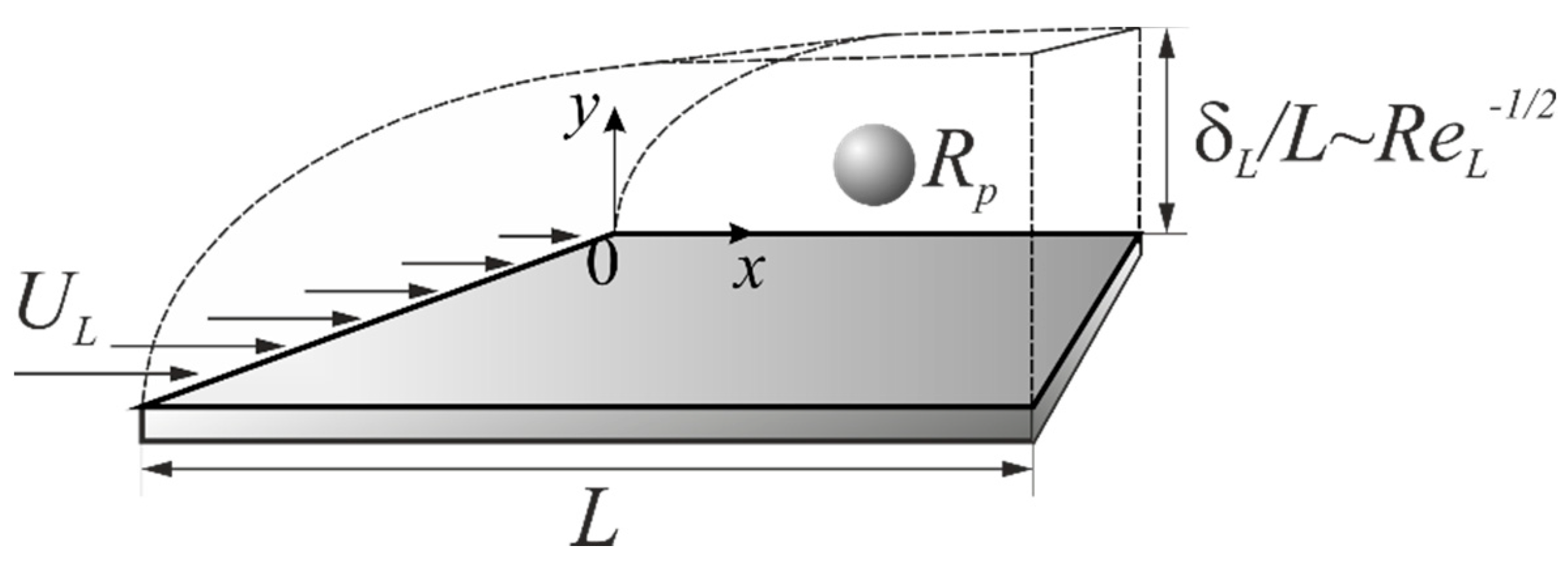
A neutrally buoyant solid sphere of radius Rp, is situated in a BL at a solid plate of length L. The model situation is sketched in Figure 1. The characteristic thickness of the BL region at the plate is , where is the Reynolds number and UL and ν are the flow velocity and the kinematic viscosity of the fluid, respectively [11] (p. 126). The sphere perturbs the outer BL flow at the plate due to its finite dimensions Rp. The basic parameter ratios that characterize the perturbation flow field are δL/L << 1, Rp/L<<1, and Rp/δ < [12,13,14,15]. There geometric interrelations allow to perform a scaling analysis for the governing Navier–Stokes equations [16,17] of the disturbance flow field, so that a system of asymptotic hydrodynamic equations is obtained, which can be solved analytically. Then, the overall force acting on the solid sphere is calculated. Finally, the particle trajectories within the BL are obtained.
The procedure is the following: the total perturbed field around the rigid sphere is presented as a sum of the “empty” BL flow and a disturbance flow field (Equations (1) and (2)):
vt= ve+ vd
pt = pe + pd.
The indexes “t,” “e,” and “d” stand for velocity and pressure of total, external, and disturbance fields, respectively. Bold style denotes vector quantities. The total flow field (vt, pt) satisfies the stationary equations of Navier–Stokes (Equations (3) and (4)):
where μ is the dynamic fluid viscosity and ρ is the density of the fluid. Upon substitution of Equations (1) and (2) in Equations (3) and (4) and taking into account that the external flow field (ve, pe) also satisfies the stationary Navier–Stokes equations, the following system of equations that governs the hydrodynamic interaction sphere/BL is obtained:
These are nonlinear second-order partial differential equations, for which analytical solution do not exist [18]. However, based on the parameter ratios, the model Equations (5) and (6) may be further simplified. The approach is to introduce the appropriate scaling parameters so as to render the respective quantities dimensionless and to convert Equations (5) and (6) into a system of successive approximations. First, if a rigid neutrally buoyant sphere is inside the BL region at the wall, there is one cause for the perturbation of the external BL flow: the deformation of the flow field due to the finite size of the solid, as compared to the characteristic BL thickness δL. Faxen studied a similar type of interaction [19,20]. He established that in a Stokes-type external flow, an additional drag on the particle with regard to the velocity of the external flow appears [21]. The so-called Faxen’s deformation velocity vF [21] is presented as Equation (7):
where the index “e” refers to external flow characteristics. The subscript “O” denotes that the magnitudes are taken at the point where the center of the sphere is situated.
Second, for any particle that lags behind of the basic flow, an additional hydrodynamic interaction appears. This is often referred to as lateral migration and was initially studied by Saffman [22,23]. The nature of this phenomenon is related to a combined action of viscous and convective hydrodynamic effects–“Saffman’s migration effect.” The respective velocity of migration may be presented as Equation (8):
Here, is the velocity of the background BL flow, is the lag velocity of the particle (the difference of the particle’s velocity and that of the external flow at the point where the particle center is situated), ν = μ/ρ is the kinematic viscosity, and i, j are coordinates. The lagging behind here is due to the deformation viscous interaction and one may assume that [5]. So, the respective quantities in the Equations (5) and (6) are scaled in the following manner (Equation (9)):
Further on, the notations are used for the dimensionless velocity and length components along the Ox and Oy axes, respectively.
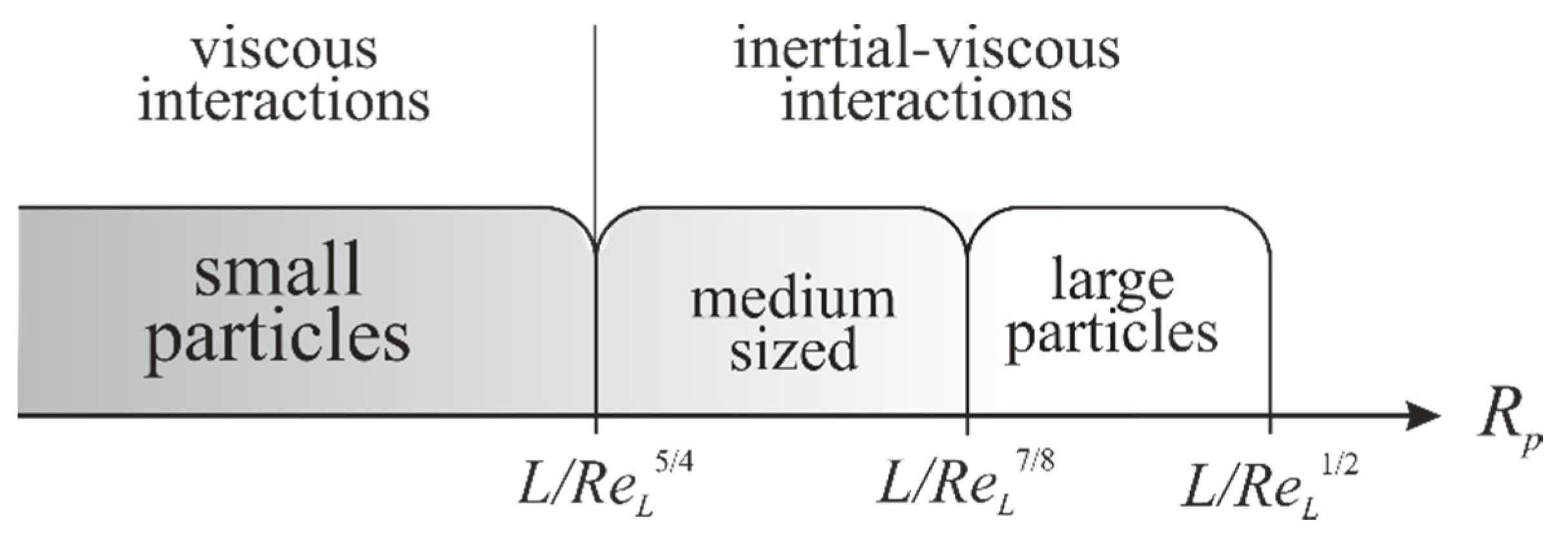
As shown in [12,13], the main result of this asymptotic analysis is that the neutrally buoyant particles are subjected to a granulometric separation inside the hydrodynamic BL at a plate as shown in Figure 2. The criterion for this classification is based on the ration of the parameters of the external flow field and particle’s dimension. Thus, interactions for the small particles with the external flow are predominantly viscous, for the medium-sized , of mixed inertial-viscous type, and for the large species , of inertial type.
The medium- and large-sized particles in a laminar BL at a plate have been experimentally investigated in [24]. The authors have shown that such species are just expelled outside the BL. Major entrapment effects inside the BL domain are obtained only for the small species, namely,. So, the scaling analysis for small particles results in the following asymptotic equation for the longitudinal () component of the disturbance velocity [14] (Equation (10)):
with the following boundary conditions (Equations (11) and (12)):
The analytical solution for the system of Equations (10)–(12) is:
The results for the transversal () component of the velocity of the disturbance field and for the disturbance component of the pressure are, respectively (Equations (14) and (15):
The total force (F) acting on the sphere is calculated according to the following expression [25] (Equation (16)):
Sp is the surface of the sphere, is the total stress tensor, and is the symbol of Kronecker. Finally, the following relations are used so as to obtain the particle trajectory ((Equations (17) and (18)):
ρ denotes the density of the particle (in the case of neutrally buoyant particle, its density is equal to that of the fluid); rp is its radius-vector of the particle center. The system of Equations (17) and (18) is solved under the following initial conditions for the coordinates of the particle center (xp, yp):
The notations () denote the dimensionless longitudinal and transversal velocity components of the particle; () are the dimensionless coordinates of the particle’s center.
2.2. Numerical Results and Discussion
Equations (17) and (18) are solved numerically and the result is presented as a function ; the latter is used to calculate the particle residence time (τ) inside the BL region [10]. The numerical experiments are performed for different plate dimensions (lengths) and various Reynolds numbers of the background fluid flow. In Table 1 are presented the dimensions of the largest solids that fulfil the demand of being small as compared to the BL thickness in each case, namely, Rp < L/ReL5/4, so as to correspond to the demands of the asymptotic model.
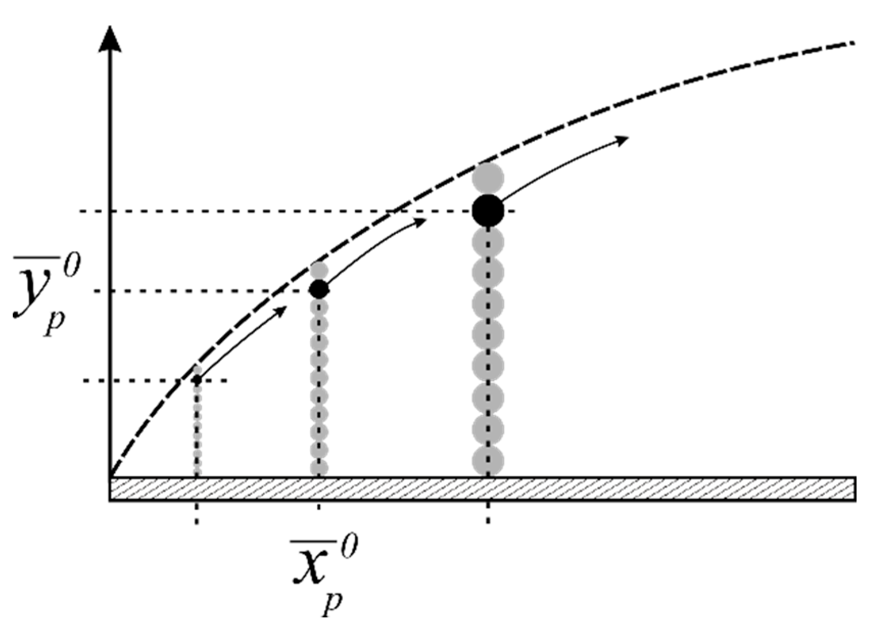
As expected, the shortest plates retain the smallest solids inside the BL; the longer the plates, the larger are the entrapped particles. For example, a plate with L = 100 cm can entrap species of the order of Rp ~ 50 mm. Having this in mind, the particles’ trajectories are calculated with the assumption that the solids are completely immersed inside the BL. The initial values of 0 for the exemplary
calculations of the trajectories are chosen to be inside the BL, as far as
possible remote from the plate (the particle center is situated three radii
inside the BL). Thus, the minimum entrapment effect for a given particle size
is estimated and thus the lower limit of residence time for each type of
particle entrapped inside the BL region is estimated. If the particle is placed
deeper towards the plate the disturbance of the background fluid flow is much
higher. The choice is schematically illustrated in Figure 3.
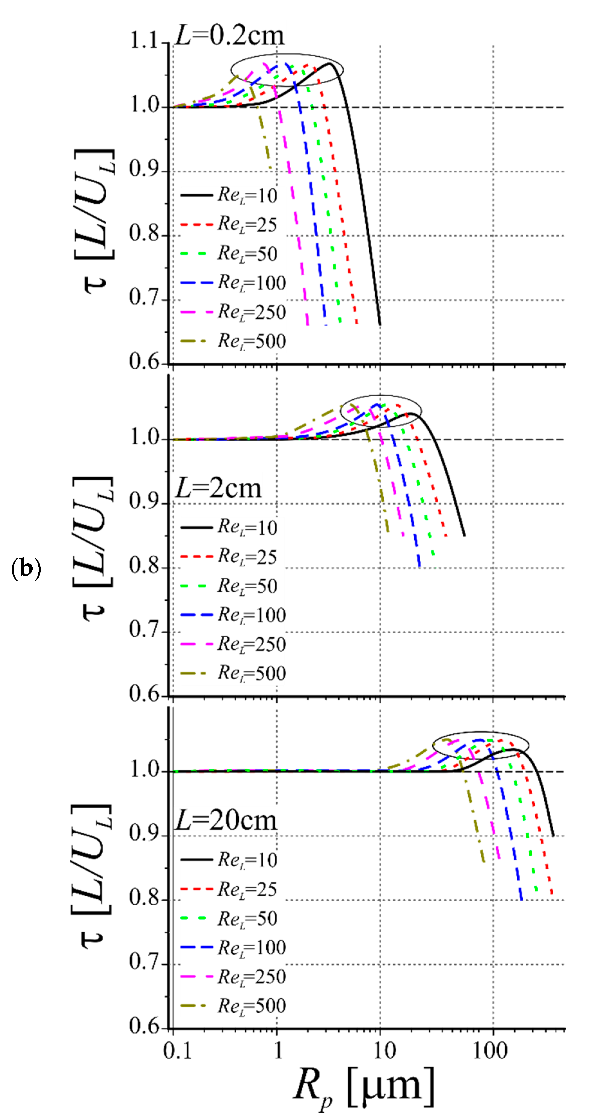
The results about the residence time for various particle’s radii Rp of the solid spheres and for several cases of plate’s lengths L are presented in Figure 4. The runs of the curves τ (Rp) in Figure 4a show that for the given external BL conditions, there is a range of particle’s dimensions for which the residence time inside the BL is maximal. This effect evidences that the hydrodynamic boundary layer in the vicinity of the solid wall has a substantial potential for granulometric separation of polydisperse solids along the BL thickness. In addition, this is an exclusive effect of the finite dimensions of the species entrapped in the BL. Moreover, there are two additional characteristics of the spectra, as shown in Figure 4b: (i) for each value of L, the maximum in the residence time is shifted towards smaller particles at the increase in ReL. Therefore, more intensive BL flow is particularly effective in the granulometric separation of the finest solids, while larger particles are entrapped and classified in size within a less intensive BL (higher value of δL). (ii) Upon increase in L (for all ReL as shown in Figure 4b), the maxima in the residence times are shifter towards larger entrapped species. So, longer plates are more effective in the granulometric separation of larger particles, while more detailed size classification is expected in BL at shorter plates.
The run of τ(Rp) for various length L, but at fixed Reynolds number ReL is presented in Figure 5. The results support the conception that the medium values of the Reynolds number of the background BL flow and the shorter plates are most effective in the granulometric separation of a wider range of fine species, while only the smallest particles could be entrapped within the BL regions of higher Reynolds numbers.
In conformity of this notion are also the data summarized in Figure 6a. Figure 6a presents the interrelation of particles sizes that have maximum residence times inside the BL flow (the values are taken from the maxima in the spectral curves τ (Rp) in Figure 4a,b) against the plate lengths Rp(L) for various ReL. The key result denotes that the most effective BLs are those at ReL = 25, while the least effective, in view of particle capture efficiency, are the BLs with ReL = 500. The detailed data particularly for the finest species and smaller plates, are demonstrated in Figure 6b. This presentation allows to predict, say, the optimal dimensions of the plate at which the hydrodynamic BL is formed. For example, the idea about the conditions for possible granulometric separation of neutrally buoyant sphere of a given radius (Rp = 3 μm) may be extracted in the following manner: The intersections of the horizontal line Rp = 3 μm with each of the various Rp(L)-curves denote the respective lengths of the plates (L) that are expected to ensure the maximum capture effect for this size of the fine solid. Thus, if the Reynolds number of the background flow at the plate is ReL = 25, the optimum length of the plate is L ~ 0.3 cm, while if ReL = 100, the optimum length is L ~ 0.6 cm.
The general presentation of the obtained numerical results, in a form suitable for predictive aims about the design of separation experiments with neutrally buoyant fine entities, is shown in Figure 7 as Rp(UL).
The key outcome is that it is possible to use the hydrodynamic BLs for granulometric separation of fine submicron- and micron-sized neutrally buoyant particles when a polydisperse suspension flows in the vicinity of solid walls (plates).
3. Gravity Effects
3.1. Theoretical Background
The next step is to account for the fact that the targeted fine solids may have densities higher than the respective value of the surrounding fluid. This gravity effect might interfere with the already established granulometric separation in the vicinity of solid walls (plates). The aim here is to estimate this influence. In the model situation as presented in Figure 1, the gravity effects act along the y-axis. Therefore, in the preliminary scaling analysis, one has to account for the particle’s sedimentation velocity (vG), as well, namely Equation (22):
In Equation (22), g is the gravitational acceleration, ν is the kinematic fluid viscosity, Δρ/ρ is relative density of the particle inside the fluid (for neutrally buoyant particle, Δρ/ρ = 0.
Generally, the disturbance velocity (vd) may be scaled by: (i) Faxen’s deformation (Equation (7)), (ii) Saffman’s migration effect (Equation (8)), and (iii) sedimentation velocity (Equation (22)). In the case of neutrally buoyant particle, the velocity components are scaled either with Faxen’s deformation or with Saffman’s migration. However, for the model situation, as depicted in Figure 1, the sedimentation effect couples only with the transverse velocity component (vy). So, all possible interrelations are shown in Figure 8.
One of the challenging problems in the separation processes is the extraction of small particles. As is shown above in Section 2, for neutrally buoyant species, this means dimensions in the range of . Particular feature of the disturbance velocity components in this case is that they are of the order of magnitude of the Faxen’s deformation, both in longitudinal and transverse directions with regard to the solid wall. In the case of heavy particles, however, two option appear, for the estimation of the transverse disturbance velocity component: (i) through Faxen’s deformation velocity (vF, Equation (7)) or (ii) through the sedimentation velocity (vG, Equation (22)). Thus, the fine small () species might further be classified into light and heavy particles (Figure 8).
The modeling and the numerical calculations are further focused on the light particles. The reason is that heavy particles are not very much affected by the BL fluid flow. However, for light and small species ( and , Figure 8), the sedimentation phenomena cause additional modification to the major deformation effect within the background BL fluid flow due to the finite dimensions of the particles. Thus, the asymptotic model and the analytical solutions for the disturbance field (vd, pd) are presented as Equations (10)–(15), (see Section 2). The gravity effect, however, affects the force acting on the entrapped fine solid.
While the initial asymptotic model (Equations (17) and (18)) for the small neutrally buoyant particles () are:
For the case of light particle (), this model is transformed into:
Here, the notation “NB” stands for the respective magnitudes concerning the neutrally buoyant case (as described in Section 2). The initial conditions are as in Equations (19)–(21).
3.2. Numerical Results and Discussion
The numerical calculations are concentrated on obtaining the theoretical predictions about the residence times and the trajectories of small light particles inside the BL flow (in the vicinity of a flat wall).
The parameters used in these calculations are presented in Table 2. The values for the small species are denoted with red color (), while those for the light case are colored with blue (). Note that for L = 2 cm, the model situation is already nonapplicable. So, the present analysis concerns smaller values of L.
Figure 9 illustrates how the regions of simultaneous action of both deformation interaction and gravity are shifted for various particle’s radii, different relative densities, and several Reynolds numbers for the BL flow.
As is to be seen from Figure 9, upon rise of ReL, the region of interaction of both coupling effects is shifted towards larger L. Besides, the entrapment effect is more effective for smaller species.
The typical residence times as a function of particle’s dimensions τ(Rp) are shown in Figure 10. As taken from Table 2, the value of L is 0.2 cm, ReL = 250, and Δρ/ρ < 0.23, because in this case, a significant effect of the coupling is to be expected. As is shown in Figure 10a, upon increase in the relative density of the particle up to Δρ/ρ~0.007, the residence time of the particles increases and the maximum values are shifted to smaller species. The residence time sharply decreases for larger entities (Rp ≥ 1 mm and Δρ/ρ~0.009–0.011). At higher density values (Δρ/ρ~0.016), the entrapment of the small particles in the BL region is diminished and the particles are expulsed out of the BL. This tendency is preserved for further increase in Δρ/ρ, and at Δρ/ρ~0.04, the residence time does not depend on Rp.
The detailed trajectories of a particle with Rp = 1 μm for a range of relative densities Δρ/ρ are presented in Figure 10b. Upon increase in Δρ/ρ up to Δρ/ρ~0.007, there is an increase in the residence time within the BL. For Δρ/ρ > 0.01, the particle’s trajectory is already directed towards the plate (wall) and the possibility of its entrapment is increased, although the residence time within the BL is shortened. At even higher densities (Δρ/ρ > 0.02), the gravity effect prevails over the hydrodynamic interaction phenomena, and the particle quickly sediments on the wall.
The obtained numerical results evidence that aside the granulometric separation of fine solids, there is a possibility for density-driven segregation inside the BLs and along the solid plate, as well. The particles with highest relative densities are captured at the initial portions of the BL; this happens quickly within short residence time. Therefore, due to the simultaneous action of viscous deformation and gravity effects, particles with well-defined characteristics (Rp and Δρ/ρ) are entrapped by the BL and could be captured at various places at the wall (plate). The notion about the coupled viscous-deformation and gravity effect may be followed in the results, shown in Figure 11.
The calculations are performed for L = 0.2 cm and ReL = 250. A particle with Rp = 1 μm is taken for an example, because, as is already shown in Figure 10a,b, it is for these outer flow conditions and such radius of the particle that the residence time τ can have the highest value, if the particle is neutrally buoyant. Thus, the choice of the particle dimension is subjected to the condition that it is both small (according to the classification in Figure 2) and light (Figure 8). As is to be seen in Figure 11a, the neutrally buoyant particle (Δρ/ρ = 0.0) is retarded inside BL, but it is finally expelled out of the BL region. For nonzero relative densities (Δρ/ρ = 0.012 and Δρ/ρ = 0.226), however, it is captured at the wall. Besides, as is to be expected, the higher the density, the shorter is the region on the plate surface, where the particle is entrapped (the so-called “particle entrapment portion of the plate”). Figure 11b represents the interrelation of the range of the particle entrapment portion of the plate and the intensity of the BL flow represented by the Reynolds number ReL: the higher the relative density is, the higher ReL values are at which the fine solids can be captured by the wall. However, these phenomena have their limits and the maximum value for the particle entrapment portion at these particular length scales is at ReL~75. The area between the run of the curves Δρ/ρ(ReL) and Δx(ReL) might be applied for predictive design of separation and selective entrapment of fine species from polydisperse systems in view of various practical implementations and industrial applications.
4. Conclusions
The present study substantiates the concept that the hydrodynamic boundary layer at a solid wall (plate) may act as an entrapment region for of fine species from polydisperse systems. The results show that the basic effect is due to the disturbance introduced by solid spheres in the background fluid flow. For a neutrally buoyant entity, the type of interaction is determined by the size of the spheres as compared to the thickness of the BL region. The result is a granulometric separation of the solids inside the BL domain at the wall. In the case of non-neutrally buoyant particles, gravity interferes with the separation effect. Important factor in this case is the relative density of the solid species as compared to this of the fluid. The data show that there are preferred regions along the length of the wall where the fine solids are detained. The obtained results give a detailed picture of the coupling of the various phenomena inside the boundary layer region at the plate. The outcomes of the investigation are important for the practical assessment of the general efficiency of entrapment and segregation of fine species in the vicinity of solid walls and have high potential for further design of industrial separation processes.
Funding
This research received no external funding.
Data Availability Statement
Not Applicable.
Acknowledgments
I would like to express my sincere gratitude to Elena Mileva for the fruitful discussions and successful long-lasting collaboration.
Conflicts of Interest
The authors declare no conflict of interest.
References
- Deriaguin, B.V.; Dukhin, S.S.; Rulev, N.N. Microflotation; Chemistry: Moscow, Russia, 1986; pp. 6–59. (In Russian) [Google Scholar]
- Schulze, H.J. Hydrodynamics of bubble-mineral particle collisions. Miner. Process. Extr. Metall. 1989, 5, 43–76. [Google Scholar] [CrossRef]
- Mileva, E.; Nishkov, I. Entrainment of fine hydrophilic particles by granulometric separation. Int. J. Min. Proc. 1992, 36, 125–136. [Google Scholar] [CrossRef]
- Scheludko, A.; Varbanov, R.; Nishkov, R.; Nikolov, D. Available online: https://worldwide.espacenet.com/patent/search/family/003902452/publication/GB1553030A?q=Scheludko (accessed on 4 January 2021).
- Mileva, E. Solid particle in the boundary layer of a rising bubble. Colloid Polym. Sci. 1990, 268, 375–383. [Google Scholar] [CrossRef]
- Nikolov, L.; Mileva, E. Interaction of a solid particle with the boundary layer on a bubble. Colloids Surf. A Physicochem. Eng. Asp. 1998, 132, 81–93. [Google Scholar] [CrossRef]
- Mileva, E.; Nikolov, L. Disturbance flow field of particle inside the boundary layer on a rising bubble. Colloids Surf. A Physicochem. Eng. Asp. 1998, 132, 95–103. [Google Scholar] [CrossRef]
- Mileva, E.; Nikolov, L. Fine particle inside boundary layer on rising bubbles. Colloids Surf. A Physicochem. Eng. Asp. 2000, 168, 125–132. [Google Scholar] [CrossRef]
- Mileva, E.; Nikolov, L. Entrapment efficiencies of hydrodynamic boundary layers on rising bubbles. J. Colloid. Intref. Sci. 2003, 265, 310–319. [Google Scholar] [CrossRef]
- Nikolov, L. Hydrodynamic boundary layer at a rising air bubble and entrapment of fine solids: Gravity effects on particle–bubble interactions. J. Disper. Sci. Technol. 2018, 39, 341–348. [Google Scholar] [CrossRef]
- Schlichting, H. Grenzschicht-Theorie; Nauka: Moscow, Russia, 1974; pp. 132–141. (In Russian) [Google Scholar]
- Nikolov, L.; Mileva, E. Neutrally buoyant particle in the boundary layer at a plate. I. Viscous interaction. Colloid Polym. Sci. 1994, 272, 560–1566. [Google Scholar] [CrossRef]
- Nikolov, L.; Mileva, E. Neutrally buoyant particle in the boundary layer at a plate. II. Inertial effects. Colloid Polym. Sci. 1994, 272, 567–1575. [Google Scholar] [CrossRef]
- Mileva, E.; Nikolov, L. Disturbance flow field of a solid particle in a boundary layer along a plate. J. Disper. Sci. Technol. 1997, 18, 73–93. [Google Scholar] [CrossRef]
- Nikolov, L.; Mileva, E. Trajectories of fine particles in a boundary layer at a plate. J. Disper. Sci. Technol. 1997, 18, 95–109. [Google Scholar] [CrossRef]
- Brenner, H. Dynamics of Neutrally Buoyant Particles in Low Reynolds Number Flows. In Progress in Heat and Mass Transfer; Hetsroni, G., Sideman, S., Eds.; Pergamon Press: Oxford, UK; New York, NY, USA, 1972; Volume 6, pp. 509–574. [Google Scholar]
- van Dyke, M. Perturbation Methods in Fluid Mechanics; The Parabolic Press: Stanford, MA, USA, 1975; pp. 9–43. [Google Scholar]
- Fletcher, C.A.J. Computational Techniques for Fluid Dynamics 2, 2nd ed.; Springer: Berlin, Germany, 1988; pp. 1–46. [Google Scholar]
- Faxen, H. Der Widerstand gegen die Bewegung einer starren Kugel in einer zähen Flüssigkeit, die zwischen zwei parallelen ebenen Wänden eingeschlossen ist. Ann. Phys. 1922, 68, 89–95. [Google Scholar] [CrossRef] [Green Version]
- Faxen, H. Die Bewegung einer starren Kugel längs der Achse eines mit zäher Flüssigkeit gefüllten Rohres. Arkiv. Mat. Astron. Fysik. 1923, 17, 1–28. [Google Scholar]
- Happel, J.; Brenner, H. Low Reynolds Number Hydrodynamics; Mir: Moscow, Russia, 1976; pp. 84–90. (In Russian) [Google Scholar]
- Saffman, P.G.J. The lift on a small sphere in a slow shear flow. J. Fluid Mech. 1965, 22, 385–400. [Google Scholar] [CrossRef] [Green Version]
- Saffman, P.G.J. Corrigendum. J. Fluid Mech. 1968, 31, 624. [Google Scholar]
- Einav, S.; Lee, S. Particles migration in laminar boundary layer flow. Int. J. Multiph. Flow 1973, 1, 73–88. [Google Scholar] [CrossRef]
- Landau, L.D.; Lifshitz, E.M. Fluid Mechanics, 2nd ed.; Pergamon Press: Oxford, UK, 1987; pp. 44–49. [Google Scholar]
Figure 1.
Sketch of a spherical particle with radius Rp in the boundary layer (BL) at a plate with length L; δL is the characteristic thickness of BL.
Figure 1.
Sketch of a spherical particle with radius Rp in the boundary layer (BL) at a plate with length L; δL is the characteristic thickness of BL.

Figure 2.
Classification of particles by size and type of dynamic interaction with BL flow.

Figure 3.
Idea about the choice of the initial conditions for the trajectory calculations.

Figure 4.
Residence times of the particles against the radii τ(Rp): (a) for L = 0.2 cm and ReL = 25; (b) for three values of L (0.2, 2, and 20 cm) and various intensities of the BL flow (ReL = 10, 25, 50, 100, 250, and 500).
Figure 4.
Residence times of the particles against the radii τ(Rp): (a) for L = 0.2 cm and ReL = 25; (b) for three values of L (0.2, 2, and 20 cm) and various intensities of the BL flow (ReL = 10, 25, 50, 100, 250, and 500).


Figure 5.
Residence times of the particles against the radii τ (Rp) for various L values: (a) for ReL = 25 and (b) for ReL = 250.
Figure 5.
Residence times of the particles against the radii τ (Rp) for various L values: (a) for ReL = 25 and (b) for ReL = 250.

Figure 6.
The size (Rp) of the particles, which reside for maximal times inside the BLs at plates with various lengths (L). (a) for all cases, calculated within the investigated model situation and (b) only for the finest species (small Rp).
Figure 6.
The size (Rp) of the particles, which reside for maximal times inside the BLs at plates with various lengths (L). (a) for all cases, calculated within the investigated model situation and (b) only for the finest species (small Rp).

Figure 7.
The interrelations between the dimensions of neutrally buoyant particles Rp against the flow velocity UL for various length values of the plate L.
Figure 7.
The interrelations between the dimensions of neutrally buoyant particles Rp against the flow velocity UL for various length values of the plate L.

Figure 8.
Classification of non-neutrally buoyant particles within the boundary layer at a solid wall; is the Froude number; is the Reynolds number of the background fluid flow.
Figure 8.
Classification of non-neutrally buoyant particles within the boundary layer at a solid wall; is the Froude number; is the Reynolds number of the background fluid flow.

Figure 9.
The shift of the coupling between the deformation viscous lagging inside the BL flow and the gravity effect for the interrelations Rp(L) and Δρ/ρ(L), for small particles, and at several Reynolds numbers of the background BL flow.
Figure 9.
The shift of the coupling between the deformation viscous lagging inside the BL flow and the gravity effect for the interrelations Rp(L) and Δρ/ρ(L), for small particles, and at several Reynolds numbers of the background BL flow.

Figure 10.
(a) Typical run of the curves τ(Rp) for small and light particles. (b) Typical trajectories for a particle with Rp = 1 μm for a range of relative densities. The black dashed line concerns the case of neutrally buoyant fine particles.
Figure 10.
(a) Typical run of the curves τ(Rp) for small and light particles. (b) Typical trajectories for a particle with Rp = 1 μm for a range of relative densities. The black dashed line concerns the case of neutrally buoyant fine particles.

Figure 11.
Entrapment of small light particle with Rp = 1 μm at a plate of L = 0.2 cm. (a) Particle trajectories for various relative densities, at ReL = 250; NB means neutrally buoyant sphere. (b) The effect of Δρ/ρ at various Reynolds numbers ReL.
Figure 11.
Entrapment of small light particle with Rp = 1 μm at a plate of L = 0.2 cm. (a) Particle trajectories for various relative densities, at ReL = 250; NB means neutrally buoyant sphere. (b) The effect of Δρ/ρ at various Reynolds numbers ReL.


Table 1.
Maximum dimensions for small neutrally buoyant particles (Rp < L/ReL5/4) in boundary layer (BL) at solid plates of various length values.
Table 1.
Maximum dimensions for small neutrally buoyant particles (Rp < L/ReL5/4) in boundary layer (BL) at solid plates of various length values.
| L = 0.2 cm | L = 0.5 cm | L = 1 cm | L = 2 cm | L = 5 cm | L = 10 cm | L = 20 cm | L = 50 cm | L = 100 cm | |
|---|---|---|---|---|---|---|---|---|---|
| ReL | Rp (μm) | Rp (μm) | Rp (μm) | Rp (μm) | Rp (μm) | Rp (μm) | Rp (μm) | Rp (μm) | Rp (μm) |
| 10 | 112 | 281 | 562 | 1125 | 2812 | 5623 | 11247 | 28117 | 56234 |
| 25 | 36 | 89 | 179 | 358 | 894 | 1789 | 3578 | 8944 | 17889 |
| 50 | 15 | 38 | 75 | 150 | 367 | 752 | 1504 | 3761 | 7521 |
| 100 | 6 | 16 | 32 | 63 | 158 | 316 | 632 | 1581 | 3162 |
| 250 | 2 | 5 | 10 | 20 | 50 | 101 | 201 | 503 | 1006 |
| 500 | 1 | 2 | 4 | 8 | 21 | 42 | 85 | 211 | 423 |
Table 2.
Values about the Reynolds numbers of the background BL flow, particle’s parameters for the entrapped entities: small–; light–. Only three plate lengths are chosen, namely, L = 0.2, 0.5, and 1 cm.
Table 2.
Values about the Reynolds numbers of the background BL flow, particle’s parameters for the entrapped entities: small–; light–. Only three plate lengths are chosen, namely, L = 0.2, 0.5, and 1 cm.
| L = 0.2 cm | L = 0.5 cm | L = 1.0 cm | L = 2.0 cm | |||||
|---|---|---|---|---|---|---|---|---|
| ReL | Rp (μm) | Rp (μm) | Rp (μm) | Rp (μm) | ||||
| 10 | 112 | 0.0018 | 281 | 0.00012 | 562 | 0.000015 | 1125 | 0.000002 |
| 25 | 36 | 0.007 | 89 | 0.00046 | 179 | 0.00006 | 358 | 0.000007 |
| 50 | 15 | 0.002 | 38 | 0.0013 | 75 | 0.00016 | 150 | 0.00002 |
| 100 | 6 | 0.006 | 16 | 0.004 | 32 | 0.0005 | 63 | 0.00006 |
| 250 | 2 | 0.23 | 5 | 0.015 | 10 | 0.0018 | 20 | 0.0002 |
| 500 | 1 | 0.64 | 2 | 0.04 | 4 | 0.005 | 8 | 0.0006 |
Publisher’s Note: MDPI stays neutral with regard to jurisdictional claims in published maps and institutional affiliations. |
© 2021 by the author. Licensee MDPI, Basel, Switzerland. This article is an open access article distributed under the terms and conditions of the Creative Commons Attribution (CC BY) license (http://creativecommons.org/licenses/by/4.0/).
Share and Cite
MDPI and ACS Style
Nikolov, L. Hydrodynamic Boundary Layers at Solid Wall—A Tool for Separation of Fine Solids. Colloids Interfaces 2021, 5, 11. https://0-doi-org.brum.beds.ac.uk/10.3390/colloids5010011
AMA Style
Nikolov L. Hydrodynamic Boundary Layers at Solid Wall—A Tool for Separation of Fine Solids. Colloids and Interfaces. 2021; 5(1):11. https://0-doi-org.brum.beds.ac.uk/10.3390/colloids5010011
Chicago/Turabian StyleNikolov, Ljubomir. 2021. "Hydrodynamic Boundary Layers at Solid Wall—A Tool for Separation of Fine Solids" Colloids and Interfaces 5, no. 1: 11. https://0-doi-org.brum.beds.ac.uk/10.3390/colloids5010011