
Driven Transport of Dilute Polymer Solutions through Porous Media Comprising Interconnected Cavities


1
Department of Bioengineering, University of Illinois at Urbana-Champaign, Urbana, IL 61801, USA
2
Department of Chemical & Biomolecular Engineering, National University of Singapore, Singapore 117585, Singapore
*
Author to whom correspondence should be addressed.
Colloids Interfaces 2021, 5(2), 22; https://0-doi-org.brum.beds.ac.uk/10.3390/colloids5020022
Submission received: 3 February 2021
/
Revised: 3 April 2021
/
Accepted: 6 April 2021
/
Published: 8 April 2021
(This article belongs to the Special Issue Locomotion of Colloidal Particles)
Abstract
:Driven transport of dilute polymer solutions through porous media has been simulated using a recently proposed novel dissipative particle dynamics method satisfying the no-penetration and no-slip boundary conditions. The porous media is an array of overlapping spherical cavities arranged in a simple cubic lattice. Simulations were performed for linear, ring, and star polymers with 12 arms for two cases with the external force acting on (I) both polymer and solvent beads to model a pressure-driven flow; (II) polymer beads only, similar to electrophoresis. When the external force is in the direction of a principal axis, the extent of change in the polymers’ conformation and their alignment with the driving force is more significant for case I. These effects are most pronounced for linear chains, followed by rings and stars at the same molecular weight. Moreover, the polymer mean velocity is affected by its molecular weight and architecture as well as the direction and strength of the imposed force.
1. Introduction
Driven transport of polymers in confined geometries by means of an imposed flow or electric field is encountered in numerous applications including enhanced oil recovery [1], DNA electrophoresis in gels [2] and micro-fabricated devices [3,4], micro-fluidic flows [5] and chromatography [6]. Consequently, there has been a long-standing interest in understanding the effects of the magnitude of the driving force and polymer-wall hydrodynamic interactions (HI) upon the size, conformation, rate of transport and spatial distribution of confined macromolecules. Coarse-grained computer simulation techniques such as Langevin dynamics (LD), Brownian dynamics (BD), Dissipative Particle Dynamics (DPD), Stochastic Rotation Dynamics (SRD) and Lattice Boltzmann method (LB) are particularly suitable for such investigations as the characteristic length and time scales associated with the dynamics of the solvent and polymer chains differ by several orders of magnitude [7]. In addition to facilitating the interpretation of experimental results, such models are also capable of predicting novel phenomena that can be subsequently verified experimentally [8,9,10].
Most previous studies have focused on the transport of linear, flexible polymers in simple geometries such as slits or tubes. For example, Fan et al. [11] used DPD simulations to show that the velocity profile of a dilute polymer solution flowing through a channel can be fitted to a power law curve. Subsequently, they performed DPD simulations of a the flow of a dilute DNA solution though flat and periodic contraction and diffusion channels [12]. The molecular conformation was found to depend upon the channel geometry as well as its instantaneous position relative to the walls. Millan et al. [13] studied pressure-driven flow of dilute polymer solutions in nanoscale slit pores using DPD. The extent of deviation of the velocity profile from parabolic was found to increase with chain length and concentration. The chains were observed to migrate towards or away from the walls depending upon their length. The DPD model used in that study was later extended by Millan and Laradji [14] to study the effect of Schmidt number (Sc) upon cross-stream migration of polymers undergoing pressure-driven flow in nanoscale slits. They observed a migration away from the walls with increasing Sc. A similar observation was reported for DPD simulations of polymer solutions undergoing shear flow in a slit [15].
The effects of polymer architecture and complex wall geometry upon the spatial distribution and transport rate of confined polymer chains have been explored in a few recent studies using DPD simulations. Li et al. [16] simulated pressure-driven flow of star polymers in a cylindrical pipe. They found that star polymers of larger functionality exhibited a greater tendency to migrate towards the centerline, resulting in a larger velocity. Posel et al. [17] investigated the flow and aggregation of rod-like proteins in slit and cylindrical pores coated with polymer brushes. In the stretched state, the polymer brushes inhibited proteins’ flow and facilitated aggregation whereas the opposite was observed for the collapsed state. Flows of polymer solutions through grooved [18] and contraction-expansion [19] channels have also been studied using BD and SRD.
All the above studies were concerned with modelling driven polymer transport in relatively simple, well-characterized geometries. Therefore, driven polymer transport through more complex geometries such as those found in porous media is still not well understood. Polymer diffusion in porous media in the absence of external forces has been previously studied, most notably in the Monte Carlo simulations of Muthukumar and Baumgartner [20,21] and the experiments of Nykypanchuk et al. [22,23,24]. Studies examining driven transport of polymers in 3D porous media are far fewer. One such study was undertaken by Zeng and Harrison [25], who investigated the mobility of DNA driven through an ordered array of spherical cavities by an electric field. They performed experiments with DNA of two different lengths and observed non-monotonic dependence of mobility on field strength. In a weak field, the mobility was smaller for the longer chains, whereas the opposite trend was observed in a sufficiently strong field.
As the above works, and most of the existing literature, were restricted to linear polymers, the effect of polymer architecture upon the transport rate remains to be clarified. Moreover, the rate of polymer transport also depends upon the nature of the driving force. As previous studies have focused exclusively upon either electric field or flow-driven transport, a systematic comparison of the transport rate in the presence of different types of driving forces is currently lacking.
The present study aims to address these gaps in the literature by applying DPD simulations to investigate the driven transport of dilute polymer solutions in 3D porous media, which consists of interconnected spherical cavities constructed through assembly of colloidal particles [6,22,25]. The geometry is more complex than those investigated in most previous studies and will be described in detail in the next section. Two scenarios are considered for the external force. In the first case, it is imposed upon both polymer and solvent beads to model a pressure-driven flow. In the second, it acts upon polymer beads only, similar to electrophoresis. Hereafter, they will be referred to as the ‘flow’ and ‘field’ cases. Three polymer architectures are considered: linear, ring, and star polymers with 12 arms. The objectives of this study include: (1) study the effect of the external force magnitude upon the polymer size by evaluating the components of the gyration tensor, (2) examine the polymer orientation by evaluating the angle between the eigenvector corresponding to the largest eigenvalue of this tensor and the direction of the external force, (3) evaluate the rate of polymer transport by comparing the velocity of the center of mass (COM) for different polymer types. The spatial distribution of macromolecules as well as their mean residence and transition times are also studied. The results are useful for design and optimization of sieving media to separate polymers of different sizes and architectures [25].
The organization of this paper is as follows. The details of the simulation methodology are described in Section 2. The effects of the nature and magnitude of the driving force upon the properties of linear polymer are examined in Section 3.1. The effect of polymer architecture is discussed in Section 3.2, and the effect of chain length and external force magnitude upon the velocity is examined in Section 3.3. A conclusion is provided in Section 4.
2. Methods
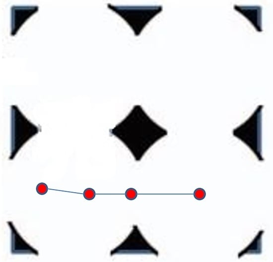
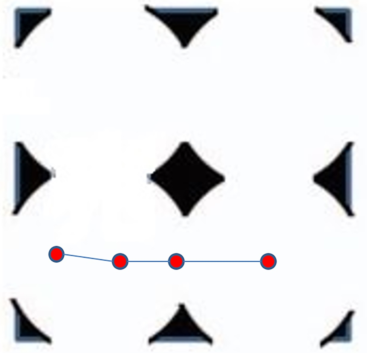
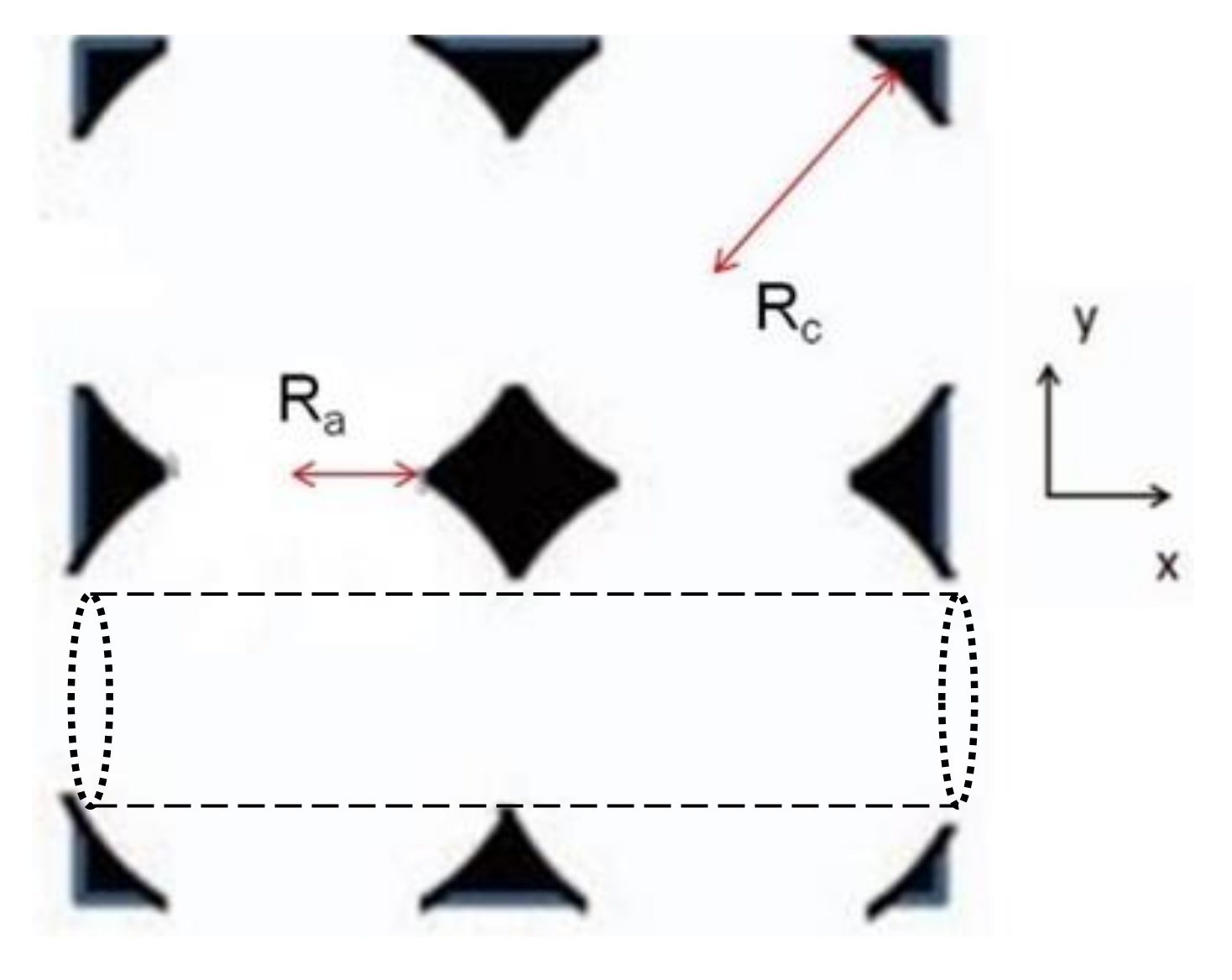
The ordered porous media consists of an array of overlapping spherical cavities arranged in a simple cubic (SC) lattice as illustrated in Figure 1. The cavity radius is designated as Rc, while the radius of the apertures connecting neighboring cavities is Ra. The medium porosity, β is given by
where h = 1/(1 − (Ra/Rc)2) [26]. In this study, the values of h and β are 1.04 and 0.56, respectively. As shown in Figure 1, the cavity array contains cylindrical channels of radius Ra connecting apertures, which are oriented parallel to the x, y, and z axes. In the absence of Brownian motion, the chains can be driven along such a channel without encountering the solid mass [26]. The effect of external force magnitude upon the localization of the polymers within these channels will be discussed in the next section.
We conduct coarse-grained simulations via DPD. Since the pairwise DPD forces satisfy Newton’s Third Law, HI are rigorously accounted for without making any pre-averaging approximation [27]. Although the Schmidt number (Sc) in a conventional DPD simulation is of O(1), which is three orders of magnitude smaller than that of a typical fluid such as water, the diffusivities and relaxation times calculated from DPD simulations of dilute polymer solutions agree with the Zimm model for both linear [28] and star polymers [16,29]. Due to its ability to accurately predict the static and dynamic properties of polymers in dilute solution, DPD is the choice of method for this study.
In the DPD method, each bead represents a cluster of atoms or molecules [30]. Each polymer molecule is modelled as a group of N beads connected by springs. The solvent and solid mass are also represented using beads. The mass of each bead and the cutoff length for the pairwise DPD forces are denoted as m and rc, respectively. As per the convention for DPD simulations, the units of mass, length, and time are chosen as m, rc and , respectively, where kB is the Boltzmann constant and T is the absolute temperature. Hereafter, all physical quantities have been normalized accordingly.
The force on a particular particle i is denoted as Fi and is given by
The force acting on each particle includes spring forces and inter-particle DPD forces that are pairwise additive and act along the line of centers of the particles. The inter-particle forces act between any two particles present in the simulation, while the spring force only acts upon the polymer beads. The finitely extendible nonlinear elastic (FENE) potential is used to describe bonded interactions:
where k is the force constant, rij is the distance between two beads i and j that are bonded to each other and R0 is the maximum allowed bond length.
The inter-particle pairwise forces are known as the conservative, dissipative and random forces denoted by , and respectively. The subscripts ‘ij’ indicate that the magnitude and direction of these forces are specific to a pair of particles. For interactions not involving wall beads, these forces were calculated using the standard expressions given by Groot and Warren [27]. The detailed forms of these expressions are given in Equations (S1)–(S4) of the Supplementary Information (SI).
For complicated geometries, methods are available to prevent mobile beads from penetrating the wall and to enforce no-slip boundary conditions at all solid-fluid interfaces [31,32]. We employed the method developed by Li et al. [33], which involves evaluating the boundary volume fraction, ϕi, for each polymer and solvent bead at each time-step of the simulation. The value of ϕi is constrained between 0 and 1 and increases as the number of wall beads located within a spherical region of radius rc centered at particle i increases. In the simulation, a predictor-corrector algorithm [33] is employed which involves performing an imaginary update of each solvent and polymer particle’s position according to and evaluating the value of ϕi(ri(t + Δt)). If ϕi(ri(t + Δt)) < 0.5, the bead is outside the wall domain. If ϕi(ri(t + Δt)) > 0.5, the particle has penetrated the wall. In this case, its original velocity is corrected according to , where en denotes the local unit normal vector of the wall boundary. Its position is then re-updated according to to avoid such penetration. In so doing, the geometry of the solid boundaries near each polymer and solvent bead is computed on-the-fly and the need to describe the shape of the solid boundaries mathematically is eliminated [33]. The no-slip boundary conditions are implemented by replacing the coefficients γ and σ in Equation (S2) with the effective coefficients γe and σe, whose values depend upon ϕi and are calculated according to Equations (6) and (12) of Li et al.’s paper [33].
Simulations without HI were also performed to understand the effect of such interactions upon the polymer properties. In these cases, the DPD dissipative and random forces, which behave jointly as a thermostat and conserve momentum due to their pairwise nature, were replaced with a Langevin thermostat, for which the dissipative and random forces act separately upon individual beads. In this case, the expressions for these forces are given as
where s is a vector with each component being a random number drawn from a uniform distribution between −1 and 1 [26]. The value of was set as 2 to ensure strong enough coupling to the heat bath such that kBT fluctuates about unity. For computational convenience, the values of ϕi were not calculated for these simulations and the standard velocity Verlet algorithm was used for time integration. Apart from these changes, the simulation protocol was identical to that employed for cases with HI.
A cubic simulation box of side length L = 20 was used with periodic boundary conditions implemented along the x, y, and z directions. It contains a single cavity whose geometric center coincides with the origin of the coordinate system. To check for finite size effects, additional simulations were performed using a larger box of side length 40 containing 8 cavities. As discussed in Section 2 of the SI, the results of these simulations are nearly identical to those obtained using a box of side length 20. Therefore, none of the results presented in the next section are expected to be affected by finite size effects.
The spring force parameters R0 and k were set to 1.50 and 30 to prevent unphysical bond crossings [34,35]. The equations of motion were integrated using the standard velocity Verlet algorithm with a time-step Δt = 0.01. The values of aij and γ were set as 18.75 and 4.5 respectively for all pairwise interactions other than those involving solid beads. The values of aij for polymer-wall and solvent-wall interactions were chosen as 150 and 120, respectively. The number of beads per chain, N, was set as 25, 37, 49, 61, or 73. For star polymers, the number of arms, f, was set to 12. In all cases, the number of polymer molecules was adjusted such that the number ratio of polymer beads to all mobile beads is as close to 0.025 as possible. As this is well below the overlap concentration, all the simulations are in the dilute regime. The value of Ra was set to 2.04 with Rc chosen as 10.21. The choice of parameter settings results in the chain conformation being similar to that in free solvent in the absence of the external force. The bead number density was selected to be 4.0 rc−3 to enable accurate evaluation of ϕi. Accordingly, the solid mass was constructed by placing 32,000 DPD particles in the simulation box, allowing them to equilibrate by means of a short DPD simulation of 2000 time steps with Δt = 0.04 and freezing the beads in the wall domain.
In all cases, the simulation began with equilibration for 500 time steps in the absence of the external force. Subsequently, an external force of magnitude Fe was imposed upon either polymer beads only or both polymer and solvent beads. In most cases, this force was directed along the positive x-direction. The value of Fe ranges between 0 and 0.14. As shown in Figure S1 of the SI, the flow within the cavity is in the laminar regime for the largest value of Fe tested. The value of Reynolds number for Fe = 0.14 is estimated to be 15.5 [12]. As most experimental investigations of flow of polymer solutions through porous media have been performed under non-inertial conditions for which Re ≪ 1 [36], the range of external force magnitude employed in our simulations is in the experimentally relevant regime.
This simulation was first run for 40,000 time steps to enable the system to reach steady state followed by a production run for up to 8 × 10⁵ time steps. The results presented for all quantities in the next section represent the average of 3 independent simulations and the error bars represent one standard deviation. The results for each simulation were obtained by averaging over 800 configurations. All simulations were performed using the Large Atomic Molecular Massively Parallel Simulator (LAMMPS) [37,38].
3. Results and Discussion
3.1. Linear Polymers
This section is concerned with the driven transport of linear polymers in cavities. The results for the flow and field cases are compared. All results presented are for N = 73.
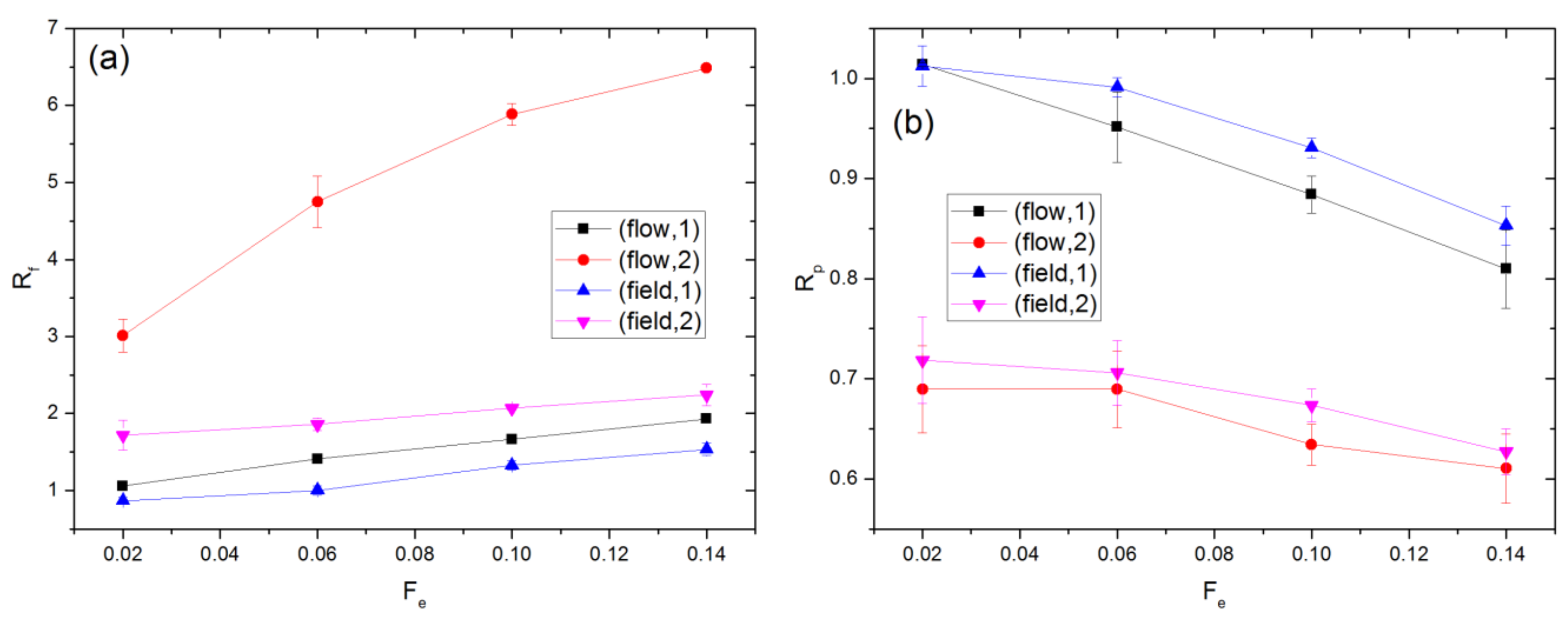
In the presence of the external force, the chains are distorted from their equilibrium conformation. The extent of this distortion is quantified by the ratios Rf and Rp, which are defined as and respectively. Here, Gαβ2 denotes the αβ components of the gyration tensor averaged over all chains and the simulation time. The subscript e denotes a property value at equilibrium (Fe = 0). The results for Rf and Rp in the flow and field cases are compared in Figure 2, where polymer molecules in one cavity are distinguished from those occupying two cavities. The value of is 3.08 ± 0.01. Since this is significantly smaller than the cavity radius, Rc = 10.21, the monomers of any polymer can be distributed over a maximum of two cavities at equilibrium. As Fe increases, the polymers’ span along the external force direction increases while that perpendicular to the external force direction decreases relative to the equilibrium value. The polymers’ average dimension along the external force direction is quantified by the value of Gxx. The maximum value of Gxx, which arises for polymers occupying two cavities in the flow case with Fe = 0.14, is 4.16 ± 0.07. As this is still significantly smaller than Rc, the polymers never occupy more than two cavities for any of the simulations performed in this study.
At equilibrium, , i.e., . With the external force imposed, Rf increases, while Rp decreases. This behavior is attributed to chain stretching, orientation change, or both. Chain stretching, which is reflected by , i.e., 2, occurs in all cases except for chains occupying one cavity in the field case with Fe = 0.02 and 0.06, where the corresponding values of 2 are 2.89 ± 0.08 and 2.98 ± 0.08. For given Fe, Rf is greater for the flow as compared to the field case, while Rp generally shows an opposite behavior. Hence, chains are distorted from their equilibrium configuration to a greater extent for the flow case. As shown in Figure S2 of the SI, the extent of this distortion is smaller in the absence of HI, indicating that such distortion is at least partly due to gradients in the solvent velocity field. For chains occupying two cavities, Rf is significantly larger for the flow case. This could be because of the shear force experienced by the chains as a result of solvent flow through the apertures.
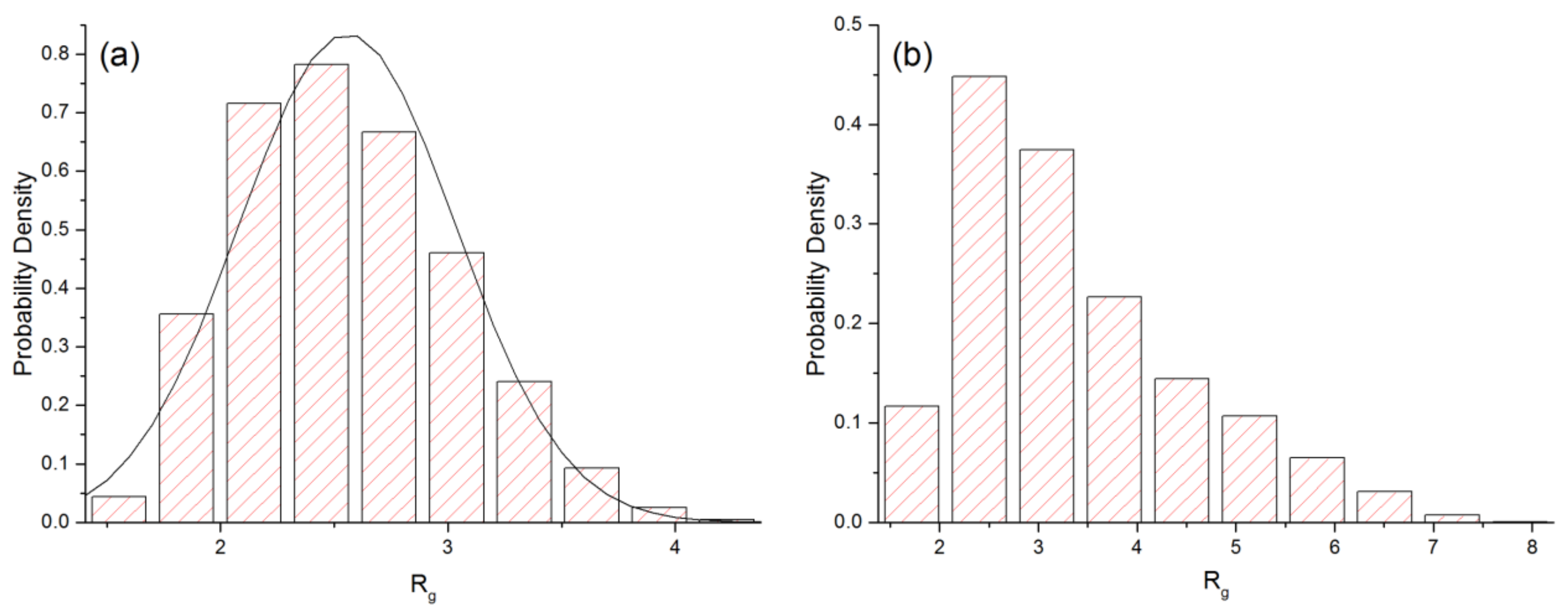
The external force not only changes the average value of Rg but also its distribution as illustrated in Figure 3 for the flow case. As Fe increases from 0 to 0.14, the mean and standard deviation of Rg increase from 2.56 to 3.36, and 0.48 to 1.16, respectively. At equilibrium, the distribution is roughly symmetric about the mean value and can be reasonably fitted to a normal distribution with a mean of 2.56 and a standard deviation of 0.48. In the case Fe = 0.14, the distribution becomes noticeably skewed. The shape of the histogram in (b) is similar to that obtained experimentally by DeLong and Hoagland [6] for a packed bed of spherical particles.
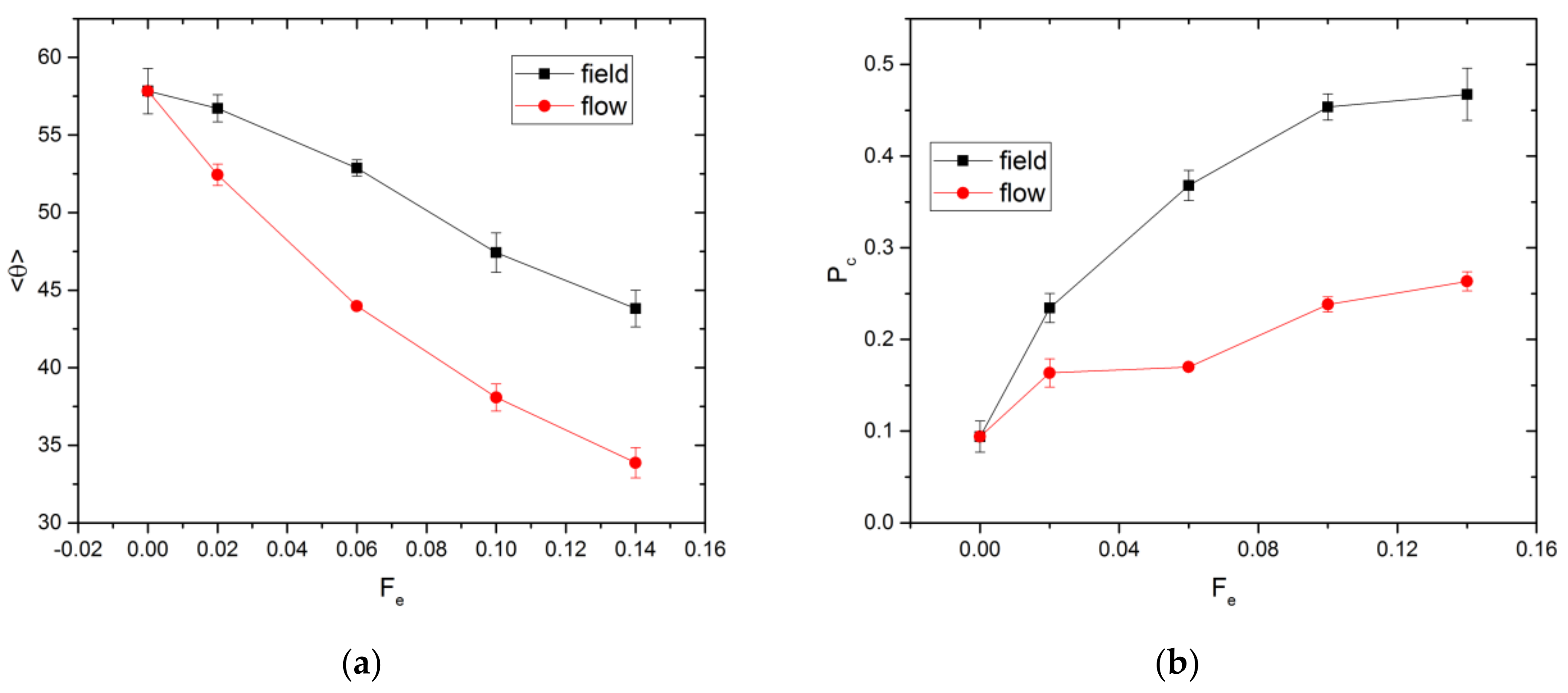
In addition to translational and stretching motion, the chains may also rotate towards the direction of the external force to reduce the hydrodynamic resistance to their movement. The degree of alignment is quantified by computing the average angle between the direction of Fe and the eigenvector corresponding to the largest eigenvalue of the gyration tensor, denoted as . If Fe = 0.0, all orientations of the eigenvector are equally probable. Since θ is constrained to lie between 0 and π/2 radian, is 1 radian, or 57.3°, as shown in Figure 4a. As Fe increases, decreases, indicative of alignment to some extent. The chain alignment is stronger for the flow as compared to the field case. In the former case, gradients in the solvent velocity field can assist the chain to rotate and align with the external force, resulting in a smaller value of . This is further verified by the flow simulations without HI, for which no significant chain alignment along the flow direction is observed (see Figure S3 of the SI). The orientation of the chains along the external force direction also increases the extent of orientational order in the system. The extent of this increase for the field and flow cases is quantified using the Saupe order tensor [39] and the results are shown in Figure S4 of the SI.
The external force alters the spatial distribution of chains within the cavity. The probability of a chain’s center of mass being located within a channel in the x-direction, Pc, is affected by the relative importance of convective to diffusive motion, which varies with Fe. Upon exiting via an aperture, a chain stays in the channel for some time before diffusing away. The effect of varying Fe upon Pc is illustrated in Figure 4b. Without an external force, the chain distribution should be uniform throughout the available space within a cavity. For a point particle, Pc is equal to the volume ratio, Vr, of the cylindrical channel to the entire cavity. This ratio is evaluated as
where the cavity volume is given by βL3. For finite-sized chains, the volume of space accessible to the center of mass is smaller than the cavity volume due to the depletion effect from the cavity wall. Hence, Pc is expected to be larger than 0.06, as observed in Figure 4b (Pc = 0.09). For nonzero Fe, Pc is significantly larger for the field as compared to the flow case.
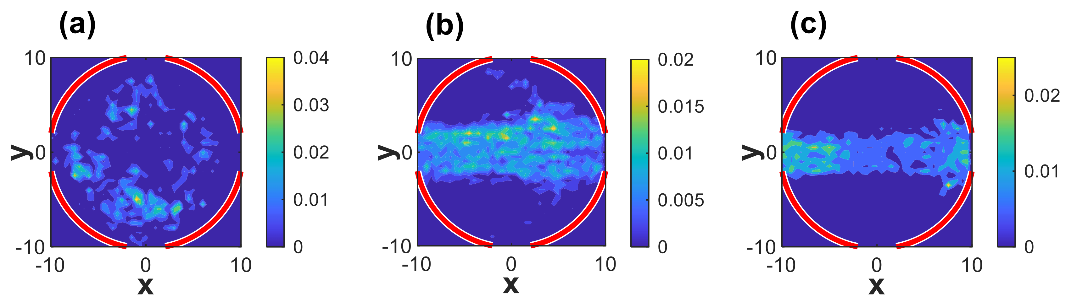
The probability density distribution of the location of the polymers’ center of mass (COM) in the x-y plane (z = 0) is plotted in Figure 5. Figure 5a shows that the COM is evenly distributed about the center of the cavity in the absence of the external force. In its presence, the polymer is largely confined within the cylindrical region indicated in Figure 1 as illustrated in Figure 5b,c for the flow and field cases, respectively. The main difference between the flow and field cases is that chains may escape from a cavity in a direction perpendicular to the external force for the former but not the latter. As shown in the velocity profile in Figure S1, some of the velocity vectors near the cavity aperture at x = −10 point away from the centerline of the cavity which is defined by y = z = 0. This gives rise to a local diverging flow that may result in the COM moving away from the centerline. Interestingly, the COM is observed to move back-and-forth between neighboring cavities along the force direction only for the field case. As such, the chain spends more time in the channels for the field as compared to the flow case, resulting in larger Pc for this case.
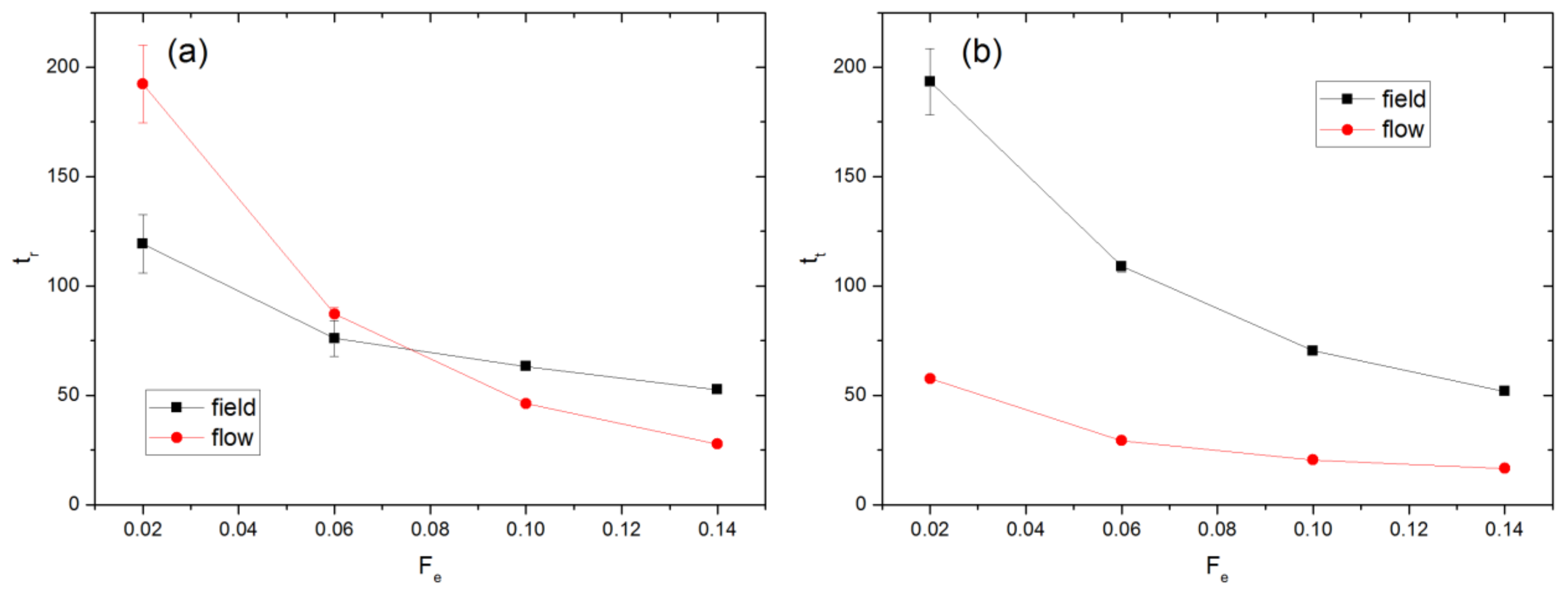
The mean values of residence time of a chain in a cavity and transition time between cavities, denoted as tr and tt respectively, are shown in Figure 6. The residence time is determined by identifying all time intervals of the simulation during which all monomers of a polymer are confined within a single cavity without entering neighboring cavities. The lengths of these intervals are then averaged for all polymers in the simulation. Similarly, all periods during the simulation in which the polymer continuously occupies 2 cavities are identified. The transition time is obtained by averaging the lengths of these intervals for all polymers in the simulation. For the investigated range of Fe, tt is always smaller than tr for the flow case, while the opposite is observed for the field case except for Fe = 0.14 where the two times become almost equal. For Fe ≤ 0.06, tr is greater for the flow case while the opposite is observed for Fe ≥ 0.10. However, tt is always greater for the field case, indicating that chain passage through an aperture is easier in the flow case. As discussed earlier, the flow can stretch and align the chains around an aperture more effectively, thereby facilitating chain escape from a cavity.
The value of tr can be used to obtain a rough estimate of the maximum distance over which a chain may diffuse perpendicular to the direction of the imposed force. For example, the value of tr for the flow case is 192.2 ± 17.7 for Fe = 0.02. The diffusivity at equilibrium, De, is (2.21 × 10⁻³) ± (1.20 × 10⁻⁴). The maximum distance through which the COM of such a chain can diffuse is approximately , which is smaller than the aperture radius Ra. Please note that Fe = 0.02 represents the smallest value of external force magnitude tested. For larger Fe, the distance over which the chains diffuse will be smaller since tr decreases as Fe increases. This analysis is consistent with the observation that Pc increases as Fe increases.
3.2. Effect of Polymer Architecture
In this section, results are presented and compared for linear, ring, and star polymers with 12 arms. Although only the flow case is illustrated, the conclusions are also applicable to the field case unless stated otherwise. We set N to be 25, 37, and 73 for linear, ring, and star polymers, respectively, because they have similar Rg,e, ranging between 1.33 and 1.39. Representative simulation snapshots of linear, ring, and star polymers in each state are shown in Figures S5–S7 of the SI. Videos illustrating the motion of each type of polymer through the cavity array in the presence of a pressure-driven flow are also available.
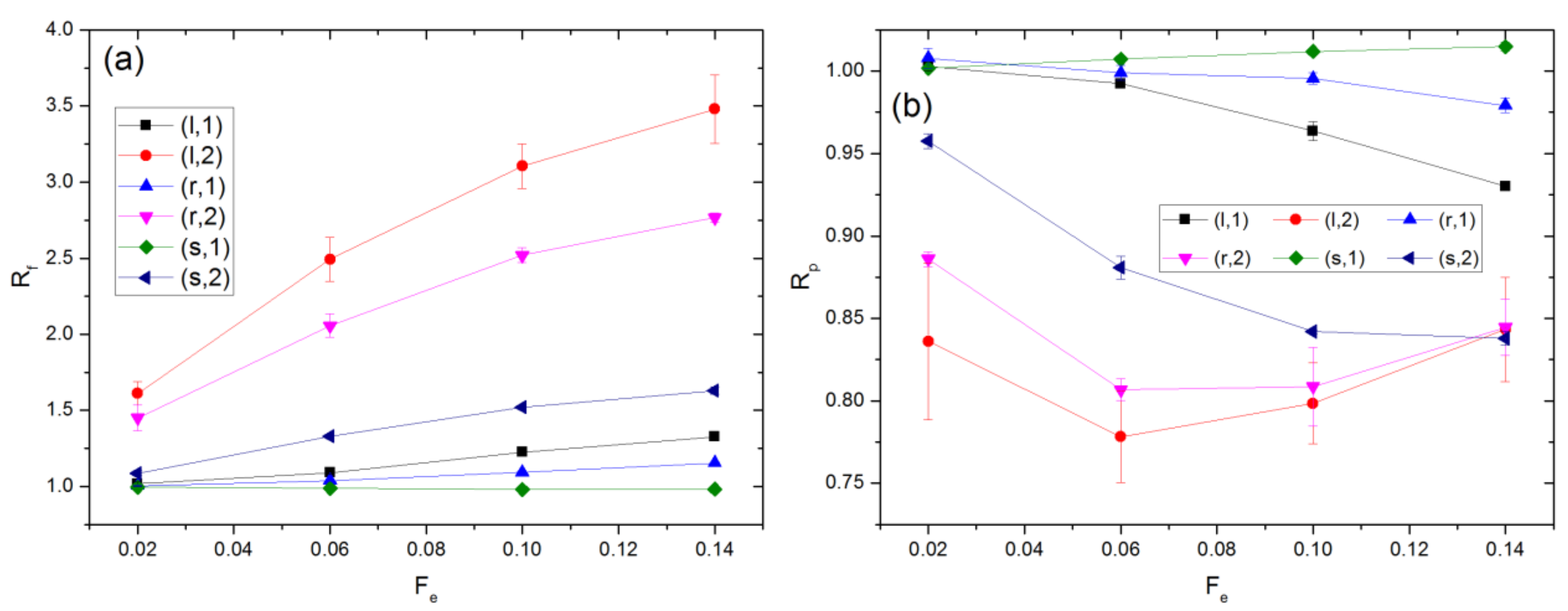
The results of Rf and Rp for different polymer types are shown in Figure 7. Their dependences on Fe are strongest for linear chains, followed by rings and then stars. For rings, the constraint of structural closure prevents them from being distorted to the same extent as linear chains. The weaker distortion experienced by stars as compared to linear polymers is primarily due to the characteristic relaxation time of the former type of polymer being significantly smaller as compared to the latter [40]. The ratio of the relaxation times of linear and star polymers can be estimated as , where f denotes the number of arms of the star polymer. This ratio is approximately 10 for the values of N and f investigated in this section. In addition, the compact structure of the star polymer hinders extension along the flow direction as it would result in overlap of arms [40].
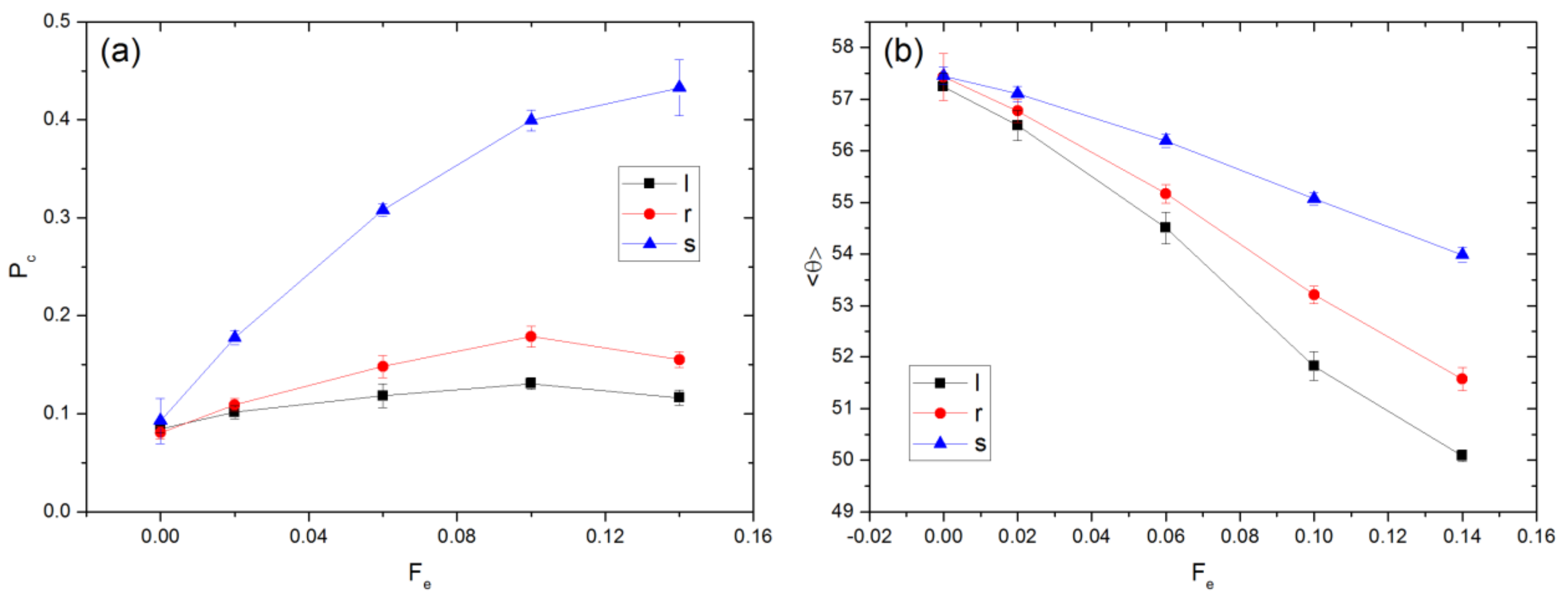
Figure 8 plots Pc and for different polymer types. As shown in panel (a), the values of Pc for the different polymer types are nearly equal at Fe = 0. Since the comparison is carried out for similar Rg,e, the volume of space accessible to the COM of polymer of each type should be similar, accounting for the above observation. As Fe is increased, Pc increases rapidly for stars but only slightly for the other two polymer types. This finding can be understood based on the fact that the strength of convection relative to diffusion is greatest for stars since they have more beads and experience the largest total external force at given Fe. This behavior shows an interesting similarity to that observed for a Poiseuille flow between parallel plates from a computational study [40], where the comparison was made for linear chains and stars with similar Rg,e,. As shown in Figure 8b, the alignment with the external force is strongest for linear chains and weakest for stars. As they are nearly spherical, stars do not have a preferred orientation even at relatively large Fe. Hence, they have a larger value of . For the values of N in Figure 8, hardly varies with Fe for the field case due to the absence of spatial velocity gradients, as shown in Figure S8 of the SI.
3.3. Velocity of COM
We now examine the effect of N and polymer type upon the average velocity of the polymer COM, denoted as v. As the results for the flow and field cases are qualitatively similar, only the results for the latter are shown.
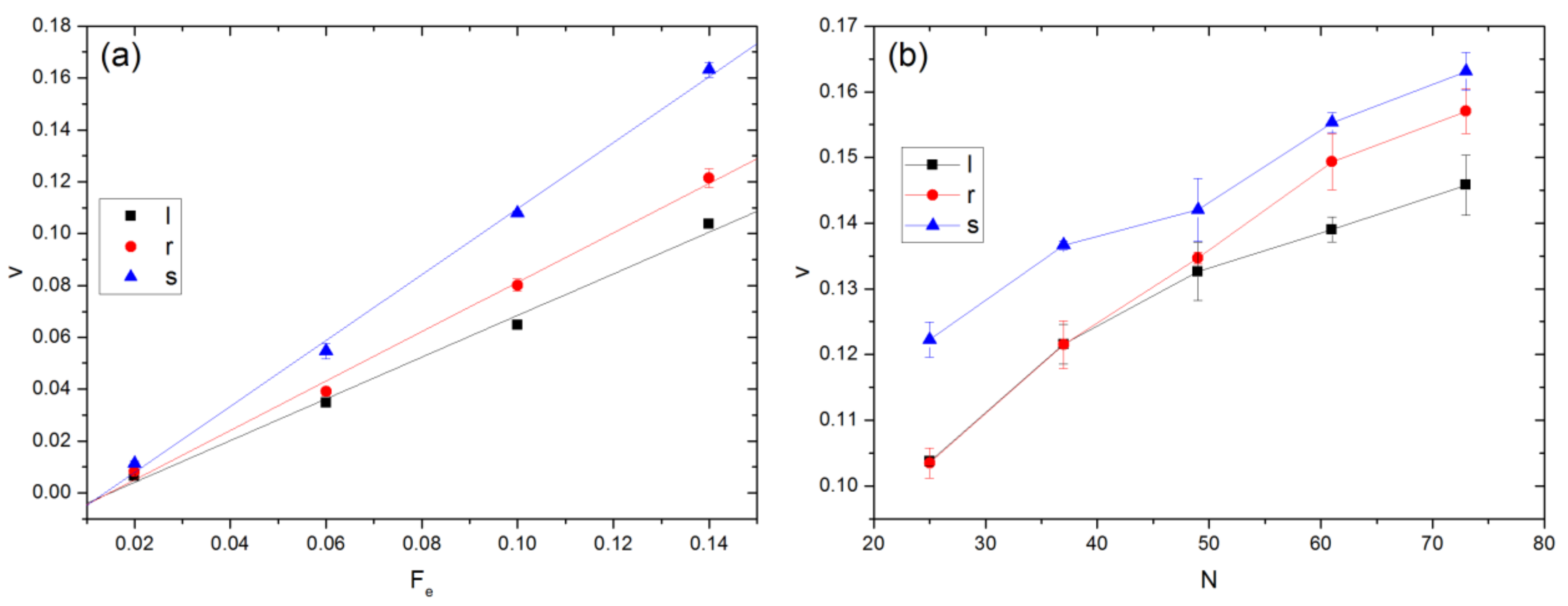
Figure 9 plots the variations of v with Fe and N. As shown in panel (a), v increases almost linearly with Fe. The mobility, which can be calculated from the slope of each curve divided by the corresponding N, is found to be 0.033, 0.026, 0.017 for linear, ring, and star polymers, respectively. Since they have similar Rge but different architectures and molecular weights, this finding indicates that driven transport in porous media is a potential method for their characterization and separation. For polymers with the same N, as seen from Figure 9b, stars still have a larger velocity than the other two types for Fe = 0.14. At equal N, Rg is smallest for stars and largest for linear polymers. There is hardly any entropic barrier effect for stars to pass through an aperture even at the largest N (=73) because Rg is smaller than Ra. However, this is not the case for linear and ring polymers when N is large enough. As shown in Figure 2 and Figure 4, linear polymers are stretched and aligned to pass through an aperture. Moreover, one can see from Figure 9b that v generally increases with N. A similar trend has been previously observed in experiments [41] and DPD simulations [42] involving electric field driven transport of DNA through a micro-channel with alternating wide and narrow regions. In such cases, it has been found that longer chains have a greater probability to escape per unit time as they have more monomers near the boundaries of the entropic traps [43,44].
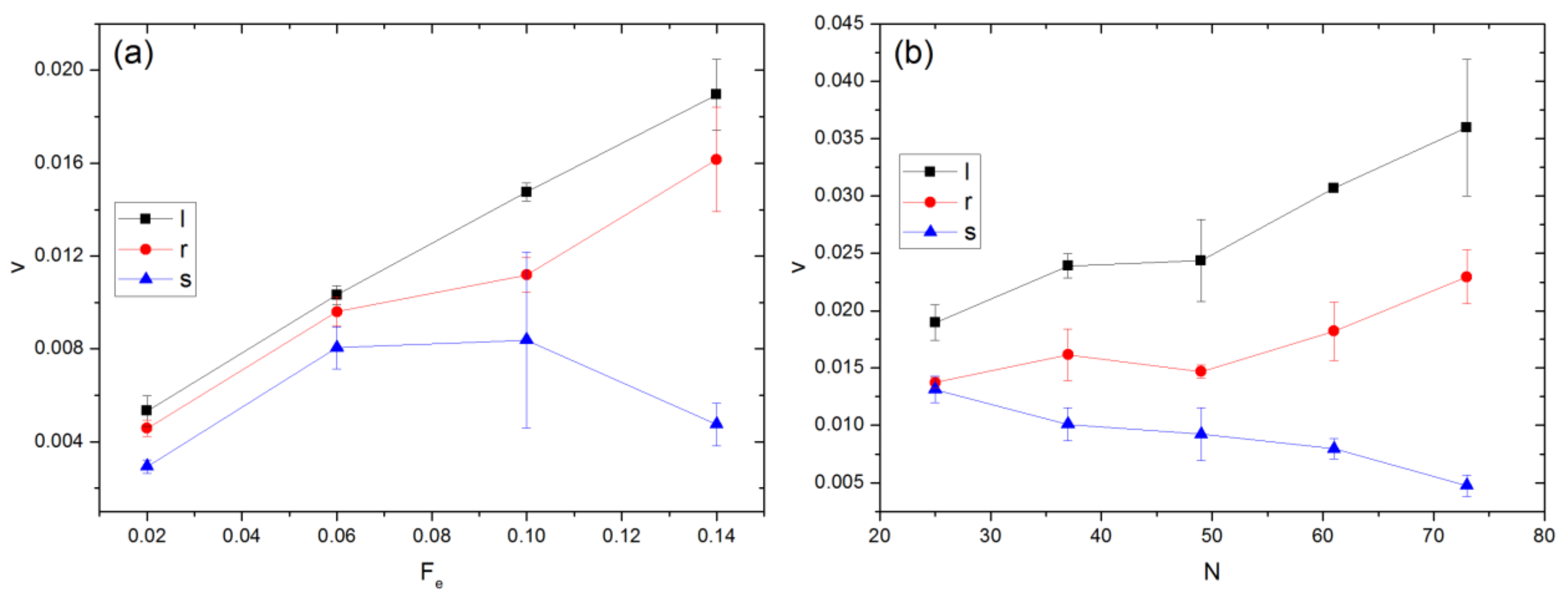
In the experiments of Zeng and Harrison [25], the electric field was applied at an angle to the principal axes along which the channels are oriented. In this case, apart from the weak entropic barrier effect, the electric field could drive some polymer segments towards the cavity wall, leading to local temporary confinement, from which they may escape via Brownian motion. To investigate these effects, simulations were performed with the external force applied at 45° from the principal axes in the x-y plane for the field case. The results are presented in Figure 10. Additional simulation results for the cases in which the external field is imposed at angles of 15° and 30° with respect to the x-axis are presented in Figure S9 of the SI. In comparison with Figure 9, v is obviously much smaller, indicative of hindrance to movement arising from the local confinement effect. It is also found that v is greatest for linear chains and smallest for stars. This behavior is opposite to the trend observed for Fe in the x-direction. As seen in Figure 10a where the polymers have similar Rge and experience entropic barriers of similar height, the difference in v between different polymer types is relatively small for Fe ≤ 0.06 but becomes significantly greater for larger Fe. As Fe increases, the confining effect of the external field becomes stronger. At given Fe, the convective effect is comparatively stronger for stars as they have the largest N and hence experience the strongest external force among the three polymer types. The increased difficulty in overcoming the local confinement can even result in v decreasing with Fe, if the latter is sufficiently large. At Fe = 0.14, as shown in Figure 10b, v decreases with N for stars but increases for the other two types. The observed behavior could be attributed to the conformation difference. The instantaneous conformation of a linear chain is a loose ellipsoidal coil, whose main dimension is larger than that of a sphere-like compact star. Because of the anisotropy, a linear polymer can change orientation due to Brownian rotation as well as interactions with the cavity wall, leading to a higher probability of accessing a nearby aperture for escape. This mechanism applies to rings but to a lesser extent. On the contrary, a spherical star is primarily driven towards the wall, as reported previously for point particles [16]. As N increases, the relative importance of convective to diffusive effect increases, leading to longer temporary entrapment of stars before escape.
4. Conclusions
The driven transport of dilute solutions of linear, ring, and star polymers with 12 arms through an array of cavities has been investigated. The distortion of the polymer conformation from the equilibrium state is greater when the external force acts upon polymer and solvent beads as compared to when it acts upon the polymer only. Also, it is strongest for linear chains, followed by rings and stars. Similarly, the extent of molecular alignment with the external force is more pronounced when this force acts upon all mobile beads, due to polymer rotation induced by gradients in the solvent velocity field. When the convection gets stronger, polymers are increasingly located in cylindrical regions that lie parallel to the direction of the external force to reduce the possibility of encountering the solid mass. The polymer average velocity increases with its molecular weight and field strength when the external force is parallel to a principal axis. For star polymers with large arm numbers, the opposite trend may be observed when the imposed field is turned away from this direction. These findings imply that driven transport through cavities is a promising method for efficient size fractionation of macromolecules. Potential avenues for future work include studying the effect of polymer rigidity, concentration, and solvent quality upon the transport rate in porous media.
Supplementary Materials
The following are available online at https://0-www-mdpi-com.brum.beds.ac.uk/article/10.3390/colloids5020022/s1, Figure S1: Velocity profile for pressure-driven flow of pure solvent through the cavity array shown in Figure 1 of the main text. The value of Fe is 0.14, Figure S2: Effect of varying Fe upon (a) Rf with HI, (b) Rf without HI, (c) Rp with HI and (d) Rp without HI. The abbreviations, l, r, and s denote linear, ring, and star polymers with 12 arms respectively, Figure S3: Angle between eigenvector corresponding to largest eigenvalue of gyration tensor and the flow direction (a) with HI and (b) without HI, Figure S4: Variation of principal order parameter, λmax with external force magnitude, Fe for field, and flow cases. The results are for a linear polymer with N = 73, Figure S5: Simulation snapshots of a linear polymer occupying (a) one and (b) two cavities, Figure S6: Simulation snapshots of a ring polymer occupying (a) one and (b) two cavities, Figure S7: Simulation snapshots of a 12 arm star polymer occupying (a) one and (b) two cavities, Figure S8: Variation of <θ> with Fe for different polymer types. The labels l, r, and s denote linear ring and star polymers with 12 arms, respectively. The corresponding values of N are 25, 37, and 73, Figure S9: Effect of ϕ upon velocity of polymers’ center of mass velocity along external field direction for the field case with Fe = 0.14. The labels l, r, and s denote linear, ring, and star polymers, respectively. The corresponding values of N are 25, 37, and 73.
Author Contributions
Conceptualization, S.B.C.; Methodology: K.N. and S.B.C.; investigation: K.N. and S.B.C.; formal analysis, K.N.; writing-original draft preparation, K.N.; writing-review and editing, S.B.C.; supervision, S.B.C.; All authors have read and agreed to the published version of the manuscript.
Funding
This work was funded by the National University of Singapore under grant number R-279-000-533-114.
Data Availability Statement
The programs used to perform the simulations in LAMMPS are available at https://github.com/nagarajankarthik/Driven-transport-of-polymers-through-porous-media (Date accessed: 7 April 2021).
Acknowledgments
The computational work for this article was partially performed on resources of the National Supercomputing Center, Singapore (http://www.nscc.sg), (Date accessed: 7 April 2021).
Conflicts of Interest
The authors declare no conflict of interest.
References
- Abidin, A.Z.; Puspasari, T.; Nugroho, W.A. Polymers for Enhanced Oil Recovery Technology. Procedia Chem. 2012, 4, 11–16. [Google Scholar] [CrossRef] [Green Version]
- Viovy, J.-L. Electrophoresis of DNA and other polyelectrolytes: Physical mechanisms. Rev. Mod. Phys. 2000, 72, 813–872. [Google Scholar] [CrossRef]
- Dorfman, K.D. DNA electrophoresis in microfabricated devices. Rev. Mod. Phys. 2010, 82, 2903–2947. [Google Scholar] [CrossRef] [Green Version]
- Dorfman, K.D.; King, S.B.; Olson, D.W.; Thomas, J.D.P.; Tree, D.R. Beyond gel electrophoresis: Microfluidic separations, fluorescence burst analysis, and DNA stretching. Chem. Rev. 2013, 113, 2584–2667. [Google Scholar] [CrossRef]
- Graham, M.D. Fluid Dynamics of Dissolved Polymer Molecules in Confined Geometries. Annu. Rev. Fluid Mech. 2011, 43, 273–298. [Google Scholar] [CrossRef]
- DeLong, C.D.; Hoagland, D.A. Imaging of Individual Polymers Undergoing Flow in a Bed of Small Spheres. Macromolecules 2008, 41, 4887–4894. [Google Scholar] [CrossRef]
- Schiller, U.D.; Krüger, T.; Henrich, O. Mesoscopic modelling and simulation of soft matter. Soft Matter 2017, 14, 9–26. [Google Scholar] [CrossRef] [Green Version]
- Slater, G.W.; Holm, C.; Chubynsky, M.V.; de Haan, H.W.; Dubé, A.; Grass, K.; Hickey, O.A.; Kingsburry, C.; Sean, D.; Shendruk, T.N.; et al. Modeling the separation of macromolecules: A review of current computer simulation methods. Electrophoresis 2009, 30, 792–818. [Google Scholar] [CrossRef]
- Ding, M.; Duan, X.; Shi, T. Flow-induced translocation of star polymers through a nanopore. Soft Matter 2016, 12, 2851–2857. [Google Scholar] [CrossRef]
- Ding, M.; Chen, Q.; Duan, X.; Shi, T. Flow-Driven Translocation of a Diblock Copolymer through a Nanopore. J. Phys. Chem. B 2019, 123, 8848–8852. [Google Scholar] [CrossRef]
- Fan, X.; Phan-Thien, N.N.; Yong, N.T.; Wu, X.; Xu, D. Microchannel flow of a macromolecular suspension. Phys. Fluids 2003, 15, 11–21. [Google Scholar] [CrossRef]
- Fan, X.; Phan-Thien, N.; Chen, S.; Wu, X.; Ng, T.Y. Simulating flow of DNA suspension using dissipative particle dynamics. Phys. Fluids 2006, 18, 063102. [Google Scholar] [CrossRef]
- Millan, J.A.; Jiang, W.; Laradji, M.; Wang, Y. Pressure Driven Flow of Polymer Solutions in Nanoscale Slit Pores. J. Chem. Phys. 2006, 126, 1–11. [Google Scholar] [CrossRef] [Green Version]
- Millan, J.A.; Laradji, M. Cross-Stream Migration of Driven Polymer Solutions in Nanoscale Channels: A Numerical Study with Generalized Dissipative Particle Dynamics. Macromolecules 2009, 42, 803–810. [Google Scholar] [CrossRef]
- Danioko, S.; Laradji, M. Tumbling, stretching and cross-stream migration of polymers in rectilinear shear flow from dissipative particle dynamics simulations. Phys. A Stat. Mech. Appl. 2012, 391, 3379–3391. [Google Scholar] [CrossRef]
- Li, Z.; Li, Y.; Wang, Y.; Sun, Z.; An, L. Transport of star-branched polymers in nanoscale pipe channels simulated with dissipative particle dynamics simulation. Macromolecules 2010, 43, 5896–5903. [Google Scholar] [CrossRef]
- Posel, Z.; Svoboda, M.; Colina, C.M.; Lísal, M. Flow and aggregation of rod-like proteins in slit and cylindrical pores coated with polymer brushes: An insight from dissipative particle dynamics. Soft Matter 2017, 13, 1634–1645. [Google Scholar] [CrossRef] [Green Version]
- Hernandez-Ortiz, J.P.; Ma, H.; de Pablo, J.J.; Graham, M.D. Concentration distributions during flow of confined flowing polymer solutions at finite concentration: Slit and grooved channel. Korea Aust. Rheol. J. 2008, 20, 143–152. [Google Scholar]
- Jiang, L.; Larson, R.G. Multiscale modeling of polymer flow-induced migration and size separation in a microfluidic contraction flow. J. Nonnewton. Fluid Mech. 2014, 211, 84–98. [Google Scholar] [CrossRef]
- Muthukumar, M.; Baumgartner, A. Effects of entropic barriers on polymer dynamics. Macromolecules 1989, 22, 1937–1941. [Google Scholar] [CrossRef]
- Muthukumar, M.; Baumgärtner, A. Diffusion of a Polymer Chain in Random Media. Macromolecules 1989, 22, 1941–1946. [Google Scholar] [CrossRef]
- Nykypanchuk, D.; Strey, H.H.; Hoagland, D. Brownian Motion of DNA Confined Within a Two-Dimensional Array. Science 2002, 297, 987–990. [Google Scholar] [CrossRef]
- Nykypanchuk, D.; Strey, H.H.; Hoagland, D.A. Single molecule visualizations of polymer partitioning within model pore geometries. Macromolecules 2005, 38, 145–150. [Google Scholar] [CrossRef]
- Nykypanchuk, D.; Hoagland, D.A.; Strey, H.H. Diffusion of circular DNA in two-dimensional cavity arrays. ChemPhysChem 2009, 10, 2847–2851. [Google Scholar] [CrossRef]
- Zeng, Y.; Harrison, D.J. Confinement effects on electromigration of long DNA molecules in an ordered cavity array. Electrophoresis 2006, 27, 3747–3752. [Google Scholar] [CrossRef]
- Chen, S.B. Driven transport of particles in 3D ordered porous media. J. Chem. Phys. 2013, 139, 074904. [Google Scholar] [CrossRef]
- Groot, R.D.; Warren, P.B. Dissipative Particle Dynamics: Bridging the Gap between Atomistic and Mesoscopic Simulation. J. Chem. Phys. 1997, 107, 4423–4435. [Google Scholar] [CrossRef]
- Jiang, W.; Huang, J.; Wang, Y.; Laradji, M. Hydrodynamic interaction in polymer solutions simulated with dissipative particle dynamics. J. Chem. Phys. 2007, 126, 044901. [Google Scholar] [CrossRef]
- Nardai, M.M.; Zifferer, G. Simulation of dilute solutions of linear and star-branched polymers by dissipative particle dynamics. J. Chem. Phys. 2009, 131, 124903. [Google Scholar] [CrossRef] [Green Version]
- Liu, M.B.; Liu, G.R.; Zhou, L.W.; Chang, J.Z. Dissipative Particle Dynamics (DPD): An Overview and Recent Developments. Arch. Comput. Methods Eng. 2014, 22, 529–556. [Google Scholar] [CrossRef] [Green Version]
- Xu, Z.; Meakin, P. A phase-field approach to no-slip boundary conditions in dissipative particle dynamics and other particle models for fluid flow in geometrically complex confined systems. J. Chem. Phys. 2009, 130, 234103. [Google Scholar] [CrossRef] [PubMed]
- Duong-Hong, D.; Phan-Thien, N.; Fan, X. An implementation of no-slip boundary conditions in DPD. Comput. Mech. 2004, 35, 24–29. [Google Scholar] [CrossRef]
- Li, Z.; Bian, X.; Tang, Y.H.; Karniadakis, G.E. A dissipative particle dynamics method for arbitrarily complex geometries. J. Comput. Phys. 2018, 355, 534–547. [Google Scholar] [CrossRef] [Green Version]
- Kremer, K.; Grest, G.S. Dynamics of entangled linear polymer melts: A molecular-dynamics simulation. J. Chem. Phys. 1990, 92, 5057–5086. [Google Scholar] [CrossRef]
- Liu, Z.; Liu, J.; Xiao, M.; Wang, R.; Chen, Y.L. Conformation-dependent translocation of a star polymer through a nanochannel. Biomicrofluidics 2014, 8, 054107. [Google Scholar] [CrossRef] [Green Version]
- Kawale, D.; Bouwman, G.; Sachdev, S.; Zitha, P.L.J.; Kreutzer, M.T.; Rossen, W.R.; Boukany, P.E. Polymer conformation during flow in porous media. Soft Matter 2017, 13, 8745–8755. [Google Scholar] [CrossRef] [Green Version]
- Plimpton, S. Fast Parallel Algorithms for Short-Range Molecular Dynamics. J. Comp. Phys. 1995, 117, 1–19. [Google Scholar] [CrossRef] [Green Version]
- Plimpton, S. LAMMPS Molecular Dynamics Simulator. Available online: http://lammps.sandia.gov/ (accessed on 1 January 2019).
- Topgaard, D. Director orientations in lyotropic liquid crystals: Diffusion MRI mapping of the Saupe order tensor. Phys. Chem. Chem. Phys. 2016, 18, 8545–8553. [Google Scholar] [CrossRef] [Green Version]
- Srivastva, D.; Nikoubashman, A. Flow behavior of chain and star polymers and their mixtures. Polymers 2018, 10, 599. [Google Scholar] [CrossRef] [Green Version]
- Han, J.; Turner, S.; Craighead, H. Entropic Trapping and Escape of Long DNA Molecules at Submicron Size Constriction. Phys. Rev. Lett. 1999, 83, 1688–1691. [Google Scholar] [CrossRef]
- Moeendarbary, E.; Ng, T.Y.; Pan, H.; Lam, K.Y. Migration of DNA molecules through entropic trap arrays: A dissipative particle dynamics study. Microfluid. Nanofluidics 2010, 8, 243–254. [Google Scholar] [CrossRef]
- Han, A.J.; Craighead, H.G. Separation of Long DNA Molecules in a Microfabricated Entropic Trap Array. Science 2000, 288, 1026–1029. [Google Scholar] [CrossRef]
- Han, J.; Craighead, H.G. Characterization and optimization of an entropic trap for DNA separation. Anal. Chem. 2002, 74, 394–401. [Google Scholar] [CrossRef]
Figure 1.
Two-dimensional representation of ordered porous media comprising interconnected spherical cavities. An example of a cylindrical channel though which a polymer can be driven without encountering the walls is shown in dashed lines in the bottom half of the figure.
Figure 1.
Two-dimensional representation of ordered porous media comprising interconnected spherical cavities. An example of a cylindrical channel though which a polymer can be driven without encountering the walls is shown in dashed lines in the bottom half of the figure.

Figure 2.
Values of (a) Rf and (b) Rp for flow and field driven transport. Chains occupying 1 and 2 cavities are treated separately. The percentage of chains occupying two cavities ranges from 15.6 to 36.8% and 17.9 to 39.4% for the flow and field cases, respectively.
Figure 2.
Values of (a) Rf and (b) Rp for flow and field driven transport. Chains occupying 1 and 2 cavities are treated separately. The percentage of chains occupying two cavities ranges from 15.6 to 36.8% and 17.9 to 39.4% for the flow and field cases, respectively.

Figure 3.
Distribution of Rg for (a) Fe = 0 and (b) Fe = 0.14 for the flow case. The curve in (a) is the fit to a normal distribution.
Figure 3.
Distribution of Rg for (a) Fe = 0 and (b) Fe = 0.14 for the flow case. The curve in (a) is the fit to a normal distribution.

Figure 4.
Values of (a) <θ> and (b) Pc for field and flow cases.

Figure 5.
Probability density distribution of location of polymers’ center of mass (COM) in x-y plane. The plots are for the cases (a) Fe = 0.0, (b) flow case with Fe = 0.14 and (c) field case with Fe = 0.14.
Figure 5.
Probability density distribution of location of polymers’ center of mass (COM) in x-y plane. The plots are for the cases (a) Fe = 0.0, (b) flow case with Fe = 0.14 and (c) field case with Fe = 0.14.

Figure 6.
Values of (a) residence and (b) transit times for field and flow cases.

Figure 7.
Effect of varying Fe upon (a) Rf and (b) Rp. In the legend, l, r, and s denote linear, ring, and star polymers, respectively; 1 and 2 denote the number of cavities occupied by the polymer.
Figure 7.
Effect of varying Fe upon (a) Rf and (b) Rp. In the legend, l, r, and s denote linear, ring, and star polymers, respectively; 1 and 2 denote the number of cavities occupied by the polymer.

Figure 8.
Effect of varying Fe upon (a) Pc and (b) for different polymer types. In the legend, l, r, and s denote linear, ring, and star polymers, respectively.
Figure 8.
Effect of varying Fe upon (a) Pc and (b) for different polymer types. In the legend, l, r, and s denote linear, ring, and star polymers, respectively.

Figure 9.
Variation in velocity of polymer COM with (a) Fe and (b) N. In (a), Rge is similar for the different polymer types, while Fe = 0.14 in (b). In the legend, l, r, and s denote linear, ring, and star polymers, respectively.
Figure 9.
Variation in velocity of polymer COM with (a) Fe and (b) N. In (a), Rge is similar for the different polymer types, while Fe = 0.14 in (b). In the legend, l, r, and s denote linear, ring, and star polymers, respectively.

Figure 10.
Variation of v with (a) Fe and (b) N. The external force acts at 45° angle from the x-axis in the x-y plane upon polymer beads only. In (a), Rge is similar for different polymer types, while Fe = 0.14 in (b). In the legend, l, r, and s denote linear, ring, and star polymers, respectively.

Publisher’s Note: MDPI stays neutral with regard to jurisdictional claims in published maps and institutional affiliations. |
© 2021 by the authors. Licensee MDPI, Basel, Switzerland. This article is an open access article distributed under the terms and conditions of the Creative Commons Attribution (CC BY) license (https://creativecommons.org/licenses/by/4.0/).
Share and Cite
MDPI and ACS Style
Nagarajan, K.; Chen, S.B. Driven Transport of Dilute Polymer Solutions through Porous Media Comprising Interconnected Cavities. Colloids Interfaces 2021, 5, 22. https://0-doi-org.brum.beds.ac.uk/10.3390/colloids5020022
AMA Style
Nagarajan K, Chen SB. Driven Transport of Dilute Polymer Solutions through Porous Media Comprising Interconnected Cavities. Colloids and Interfaces. 2021; 5(2):22. https://0-doi-org.brum.beds.ac.uk/10.3390/colloids5020022
Chicago/Turabian StyleNagarajan, Karthik, and Shing Bor Chen. 2021. "Driven Transport of Dilute Polymer Solutions through Porous Media Comprising Interconnected Cavities" Colloids and Interfaces 5, no. 2: 22. https://0-doi-org.brum.beds.ac.uk/10.3390/colloids5020022