Article

An Alternative Methodology to Compute the Geometric Tortuosity in 2D Porous Media Using the A-Star Pathfinding Algorithm

by
Mayken Espinoza-Andaluz
1,*,
Javier Pagalo
2,
Joseph Ávila
3 and
Julio Barzola-Monteses
4,5
1
Escuela Superior Politécnica del Litoral, ESPOL, Facultad de Ingeniería Mecánica y Ciencias de la Producción, Centro de Energías Renovables y Alternativas, Campus Gustavo Galindo Km. 30.5 Vía Perimetral, P.O. Box 09-01-5863, Guayaquil 090112, Ecuador
2
Escuela Superior Politécnica del Litoral, ESPOL, Facultad de Ingeniería Mecánica y Ciencias de la Producción, Campus Gustavo Galindo Km. 30.5 Vía Perimetral, P.O. Box 09-01-5863, Guayaquil 090112, Ecuador
3
Escuela Superior Politécnica del Litoral, ESPOL, Facultad de Ingeniería en Electricidad y Computación, Campus Gustavo Galindo Km. 30.5 Vía Perimetral, P.O. Box 09-01-5863, Guayaquil 090112, Ecuador
4
Department of Computer Science and Artificial Intelligence, Escuela Técnica Superior de Ingenierías Informática y de Telecomunicación, Universidad de Granada, 1807 Granada, Spain
5
Artificial Intelligence and Information Technology Research Group, University of Guayaquil, Guayaquil 090514, Ecuador
*
Author to whom correspondence should be addressed.
Submission received: 25 February 2022 / Revised: 19 March 2022 / Accepted: 24 March 2022 / Published: 2 April 2022
(This article belongs to the Section Computational Engineering)

Abstract

:
Geometric tortuosity is an essential characteristic to consider when studying a porous medium’s morphology. Knowing the material’s tortuosity allows us to understand and estimate the different diffusion transport properties of the analyzed material. Geometric tortuosity is useful to compute parameters, such as the effective diffusion coefficient, inertial factor, and diffusibility, which are commonly found in porous media materials. This study proposes an alternative method to estimate the geometric tortuosity of digitally created two-dimensional porous media. The porous microstructure is generated by using the PoreSpy library of Python and converted to a binary matrix for the computation of the parameters involved in this work. As a first step, porous media are digitally generated with porosity values from 0.5 to 0.9; then, the geometric tortuosity is determined using the A-star algorithm. This approach, commonly used in pathfinding problems, improves the use of computational resources and complies with the theory found in the literature. Based on the obtained results, the best geometric tortuosity–porosity correlations are proposed. The selection of the best correlation considers the coefficient of determination value (99.7%) with a confidence interval of 95%.

1. Introduction

Tortuosity is an intrinsic property that allows the characterization of porous media considering their morphology. It serves as a measure of the medium’s resistance when a fluid flow is passing through heterogeneous microstructures [1]. Traditionally, when the tortuosity is considered a geometric parameter, it is defined as the ratio of an effective route length to the medium’s shortest route length [2]. An effective route represents the route that starts from one end of the sample and reaches the other end. Although the shortest route length can be specified unambiguously, this does not apply to the effective route length. This route varies according to the type of transport phenomenon evaluated. Consequently, it is possible to have different kinds of tortuosity in the same system [2], such as geometric, hydraulic, and electrical, which have been extensively analyzed in the literature [3,4,5,6].
Tortuosity is widely used in multiple scientific fields. In medicine, the case of arterial tortuosity may be a sign of vascular fragility or a useful indicator of arterial problems [7]. From an energy point of view, a fuel cell presents various porous media, e.g., catalyst and gas diffusion layer. In the mentioned device, the tortuosity is crucial for evaluating different diffusion transport phenomena [8,9].
Geometric tortuosity is represented as follows:
τ g e o m e t r i c = L g L 0
In Equation (1), as in Figure 1, L0 is the shortest route length of the analyzed material (commonly the length of the straight-line size domain), and Lg is the mean of the effective routes’ length obtained by considering the void spaces in the material.
To compute an effective path, it is necessary to have a medium with void spaces. Figure 1 is used to represent this medium, as white circles can be considered as void spaces and black circles as filled spaces. The effective path L g is obtained by considering the Euclidean distance between these white circles, setting an initial and final circle. The thick lines represent the paths obtained by the Euclidean distance. The dashed lines represent the corresponding vertical and horizontal components of these paths, which is known as long as a diagonal path is followed.
Since it is necessary to search paths, it could be treated as a pathfinding problem. Several algorithms have been used to solve the required task in previous studies. In the current study, the A-star algorithm is employed. It is not the best path-search algorithm, because other methods can preprocess the map to guarantee more efficiency. Two of them are contraction hierarchies [10,11] and transit routes [12]. However, studies have declared that the A-star is a powerful tool and a well-known best-first search algorithm due to its wide application range in solving problems [13,14]. Other algorithms have been used extensively to compute geometric tortuosities, such as the direct shortest-path search [15], the skeleton shortest path [16], fast marching [17], the Dijkstra algorithm [18], and the pore centroid [19].
Nevertheless, pathfinding algorithms are not the only way to calculate geometric tortuosity since several techniques have been developed for the study of colloidal systems [20,21] that can be applied to both prepared and modified models [22,23]. Many techniques of colloidal analysis are used for the study of porous media in addition to geometric tortuosity [24,25].
The porous media studied are two-dimensional random digitally generated. The samples are binary porous media, i.e., their numerical structure is formed by zeros and ones. We selected unity to represent solid particles and zeros to void spaces. This approach is commonly used in artificial porous media computation [1,26,27]. In addition, the porous media sizes are given in pixels, and every pixel was established as 1µm. Moreover, the porous media have dimensions of 100 × 100 pixels for the efficient use of computational resources.
The open-source library of Python, PoreSpy, is used to comply with the porous media generation [26]. The porosity for this study is in the range of 0.5 to 0.90, since it covers the property of some modern materials, such as bio-based porous materials (0.70–0.95) [28], gas diffusion layers (0.55–0.80) [29], and catalyst layers (0.40–0.60) [30]. On the other hand, for porous media with porosity smaller than 0.5, the geometric tortuosity becomes challenging to estimate due to the reduction in possible paths. In two-dimensional models, it is a critical issue that is avoided by defining porosity values greater than 0.5.
Tortuosity, as a function of the porosity, is a common way of correlation in these types of studies [1]. The well-known correlation is the Bruggeman equation, used previously on electrochemical devices [19]. However, it is important to note that tortuosity depends not only on the porosity. As demonstrated in the computational study presented by Espinoza-Andaluz et al. [31], the tortuosity also depends on the particle shape of the media.
On the other hand, the methodologies are extensive due to the different types of tortuosity [1]. One of them is the hydraulic tortuosity, a flux-based property, whose numerical computation requires the simulation of dynamics fluid methods [30]. Although some tortuosities are not related to other types, previous studies established a relationship between hydraulic and geometrical tortuosity. For the same porous media structure, the hydraulic tortuosity is higher than the geometrical one [4]. The current study compares the geometric tortuosity computed using the A-star algorithm, and the hydraulic tortuosity calculated with the lattice Boltzmann method.
In studies in which the porous media are reconstructed, the elementary representative volume is initially defined [32,33]. However, the current research considers the porous media digitally created, knowing from the beginning the bulk porosity of the media. In this work, the porous media generation algorithm delivers porous media to the size and porosity previously defined. The samples are generated based on random images, assuming they represent porous media, and the tortuosity is computed. This study aims to test the A-star algorithm as an alternative to tortuosity evaluation. As mentioned and cited previously in this section, tortuosity evaluation has been carried out with pathfinding algorithms, even with different particle shapes [31,34].
The rest of the paper is divided as follows. The methodology for solving paths through the porous media with the A-star search algorithm is presented in Section 2. Results and discussions are displayed in Section 3. Finally, conclusions and future directions are presented in Section 4.

2. Materials and Methods

This section explains the methodology for solving paths through the porous media with the A-star search algorithm. Before the A-star application, the variables included in the study must be defined, and the generation process of the porous media must be explained.

2.1. Porous Media Generation

This procedure is relevant since it guarantees the application of the pathfinding algorithm. The porous media creation starts with a matrix image of random noise generated with zeroes and ones. Then, a multidimensional Gaussian filter is applied. It is implemented as a sequence of one-dimensional Gaussian filters with a kernel of sigma equal to the mean of the image’s size divided by 40 times a correction parameter named blobbiness. The sigma formulation is intended to allow images with visually acceptable solid and porous space distribution at low blobbiness values [26]. The blobbiness is the variable that controls the morphology of the porous media and falls in the 0 to 1 range. By reducing its value, larger pore diameters in the final structure are expected. Figure 2 shows a comparison between two two-dimensional porous media with different blobbiness values where the black color represents solids and white means void spaces. In the current study, the blobbiness value is established as a constant and is equal to 0.5.
A Gaussian convolution is applied to the defined kernel and the random image previously generated. The result is a normally distributed image that is converted to a uniform (flat) distribution. Therefore, the resulting image can be defined as a gray-scale matrix ψ i j ( x ) . The solid–pore interface is set up by defining an edge level value, ψ0, which falls in the 0 to 1 range. All pixel values in the last resulting image greater than the edge level are rounded to the value one and defined as the solid phase; otherwise, a value of 0 is set and defined as the pore phase, producing a set of binary values ψ ( b i n ) i j as in Carvalho et al. [32].
Therefore, the pore indicator function is written as:
χ ( x )   = { 1   if   ψ i j ( x )   ψ 0 0 if   ψ i j ( x ) < ψ 0
where χ ( x ) is used to convert the last resulting image’s gray-scale matrix into a 0/1 binary matrix. The edge level ψ 0 , in the current study, is equal to the porosity.
On the other hand, the two-dimensional porosity ϕ can be defined as the pore area divided by the total area. In two-dimensional images, it can be obtained by counting the number of pixels in the solid phase and dividing by the total number of pixels from the binarized images. Therefore, the porosity is written as [32]:
ϕ = 1 i = 1 N x j = 1 N y ψ ( b i n ) i j N x x N y
where N X and N y   are the sizes of the binarized image. Figure 3 shows a summary of the porous media generation process.

2.2. Porous Media Selection

One of the critical points in this study is the two-dimensional generated porous media considered for the computation of the parameters. This subsection presents the conditions for selecting a generated medium. Figure 4 shows the steps followed to obtain the porous media in which the geometric tortuosity is later computed.
To generate a sample, the process starts with a mold representing the generated domain’s shape. The number of pixels used in the horizontal and vertical directions is relevant for the digital generation. In the current study, a domain of 100 pixels by side has been considered, since it allows for adequate computational resources. Once the size domain is defined, the porosity range of the study is established. The common porous media found in science and engineering applications were considered to select the appropriate range of porosities. Based on the literature, some of the porosity values for media in modern materials fall in the range of 0.50–0.90, as mentioned in Section 1. The medium’s internal morphology is controlled by the blobbiness parameter, whose function is to bring closer the pixels between them by controlling the standard deviation of the Gaussian filter. A blobbiness property of 0.5 is selected to guarantee uniformity within the media. The PoreSpy library generates the medium based on the established parameters, and a possible effective path is searched. If at least one effective path between the inlet and outlet is found, the porous medium’s digital representation is saved for computing the geometric tortuosity. In the end, 540 samples were evaluated, i.e., 60 samples for every value of porosity from 0.50 to 0.90 in steps of 0.05.

2.3. Geometric Path

The porous media were constituted by a matrix of zeros and ones. As mentioned, the zeros represented the material’s void spaces, while the ones represented the solid material. To find the geometric paths, the first column of the matrix was analyzed to know the starting nodes. Nodes are represented by the pixels, the two-dimensional units that make the medium are equal to zero or one. The term “node” is conventionally used in pathfinding algorithms. The zero values are selected in the first and last columns as starting and arrival nodes, respectively. The effective paths are determined following the zero paths from the starting nodes to the arrival nodes. All arrival nodes are assigned for each starting node, as visualized in Figure 5, for each initial point, possible arrival points are assigned. This means that the last column is checked for points that have zero, which means free spaces.
Each element within the porous domain is assigned zero or one according to its nature, i.e., zero for the pore phase and one for the solid phase. The matrix elements represent the porous domain ( ξ = P o r o u s   m e d i a ), and the elements’ subscripts help to identify each node’s position. The porous media elements received the following subscripts:
ξ = ( a 11 a 12 a 1 n a 21 a 22 a 2 n a m 1 a m 2 a m n )
To find the possible paths to be analyzed in the porous media, it is required to identify the starting and arrival nodes. The connection between the starting nodes, i.e., the zero-elements belonging to the first column of the binary matrix (4), and the arrival nodes, i.e., the zero-elements occupying the last column, allows the computation of the geometric tortuosity. The connectivity between the starting and arrival nodes is found considering the intermediate zero-nodes within the domain. Since the number of possible paths for each starting node can be less or equal to the number of arrival nodes, as seen in Figure 5, the maximum number of geometric paths cannot exceed the square of the number of rows of the half-pore represented as pixels. This case can occur if both the first and final columns of the matrix are all zeros and exist as connections between their nodes.

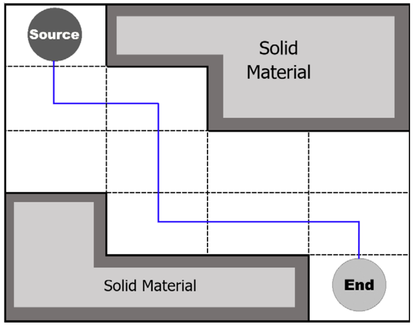
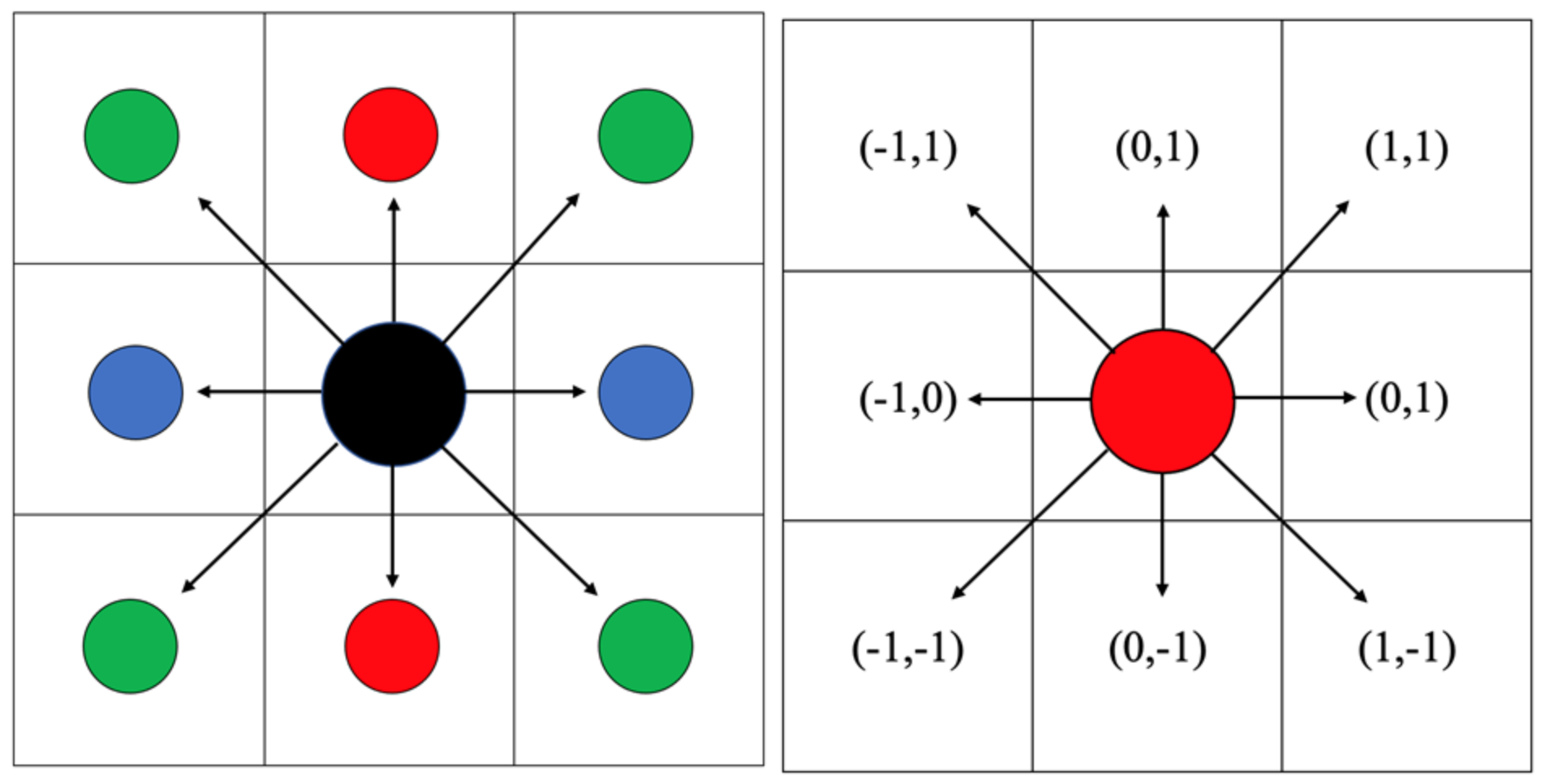
2.4. A-Star Algorithm

The A-star algorithm allows for generating an optimal path by avoiding proximity with the solid obstacle nodes.
It is a computer algorithm widely used in planning routes on a graph. A-star works similarly to Dijkstra’s algorithm, with the difference that it guides its search towards some promising states, saving computation time [35].
Figure 6 shows that the generated route can pass near the obstacles to ensure the shortest path [36].
The traditional formula applied in the A-star algorithm is expressed as:
f ( n ) = f ( x , y ) = g ( x , y ) + h ( x , y )
where 𝑓(𝑛) is the weight labeled as the node 𝑛; it can be seen as an estimation of the best path that passes through 𝑛. The real cheapest cost of obtaining the node n from the initial node is represented by 𝑔(𝑛), and ℎ(𝑛) is the so-called heuristic estimation of the cost to reach n [36]. The A-star algorithm moves in eight possible directions when applied to a two-dimensional porous medium, as shown in Figure 7.
Since the materials in this study are porous media and search-path-finding is a requirement, it was necessary to define an entry and endpoint (inlet and outlet boundaries). The entry and endpoints define the different paths followed through the domain’s void spaces. The referred paths are seen as species that can flow through the material. To determine the nodes occupied during the species’ movement, a free displacement in the four cardinal positions is considered, i.e., up, down, left, and right, as well as the ordinal positions shown in Figure 7. The simulated streamlines can flow from the inlet to the outlet. Hence, it avoids obstacles until reaching the end of the material and produces effective routes.
The measure of the effective path is carried out by calculating the Euclidean distances using Equation (5) between the ith and (i + 1)th connected nodes in the obtained path. Once the path is confirmed, a minimum value of paths for every entry node is computed, considering all the arrival nodes. The referred procedure computes effective route lengths and makes possible the calculation of 𝐿𝑔 in Figure 1. Since there are multiple possible paths, the calculation of effective routes represents intensive computational work. The number of possible paths increases according to the size of the domain and porosity of the material.
For two-dimensional regular structure meshes, the function h(x,y) is calculated with the Euclidean heuristic function:
h ( x , y ) = ( x i x j ) 2 + ( y i y j ) 2
In this case, i represents the node in the ith position, and j is used to describe the node in the (i + 1)th position.

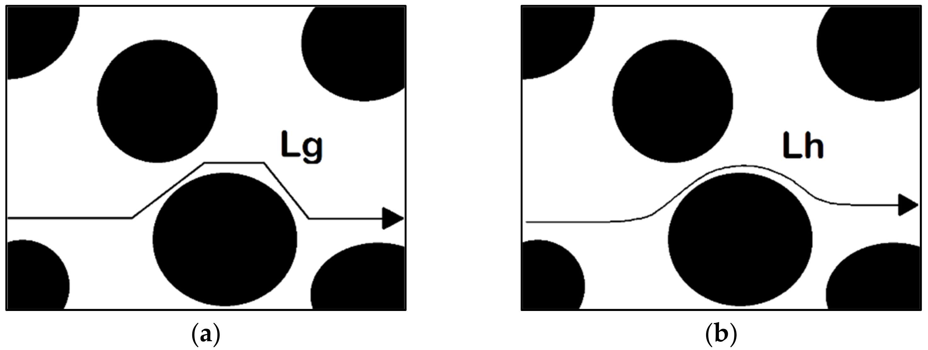
2.5. Geometric Tortuosity

To find the geometric tortuosity of a porous medium, all the possible paths based on the arrival nodes are evaluated, as depicted in Figure 5. Computing the geometric tortuosity requires finding a minimum value for all the possible paths that originated from a starting point. The evaluation was carried out on each starting node, and the computation was carried out by using Equation (7):
τ = 1 m i = 1 m [ m i n ( C i ) ] L .
where i corresponds to the index for the starting nodes, Ci is the set of paths for the starting node i, m represents the number of starting nodes, and L is the shorter length of the domain in the x-direction, equal to 100 in the current study.

2.6. Tortuosity Path

As mentioned before, there are several types of tortuosity to characterize the porous media. This section focuses on differentiating the geometric tortuosity from the others. The comparison considers the streamlines used in the geometric tortuosity and hydraulic tortuosity computation.
Geometric tortuosity: The geometric tortuosity depends on the solid material’s distribution within the domain. It can be determined as the ratio between the average length of the followed geometric paths to the straight path across an analyzed domain (side length). The geometric paths found in porous media do not follow the exact contour of solid particles. The geometric paths follow a consecutive connection of void nodes restricted to small straight lines, as shown for Lg in Figure 8a.
Hydraulic tortuosity: The complexity of a medium can also be characterized by hydraulic tortuosity. Diffusion parameters participate actively in several transport processes in porous media [7], and the hydraulic tortuosity plays a crucial role in diffusion characterization. Similar to porosity, it is also a dimensionless parameter, but it is always greater than unity. The hydraulic tortuosity is determined by solving the lattice Boltzmann equation, a powerful tool to mimic fluid behavior in complex media [37,38]:
f ( r , t ) t + c · f ( r , t ) =   Ω
where f is the particle distribution function that depends on position r, velocity c, and time t; the collision operator is represented by Ω and is a function of f. Due to the complexity of the collision term, one approximation is used to replace Ω without giving significant errors in the simulation result; this is called the Bhatnagar, Gross, and Krook (BGK) approximation. Therefore, Equation (8) is also expressed as:
f i ( r , t ) t + c i · f i ( r , t ) = 1 τ 1 [ f i e q ( r , t ) f i ( r , t ) ]
where fi(r,t) is the particle distribution function at position r and time t; f i e q ( r , t ) is the equilibrium particle distribution function, and τ 1   is the relaxation time; c i is the velocity in the corresponding i-direction.
To solve Equation (9), it is required to define the equilibrium particle distribution function f i e q ; since LBM can solve diffusion, advection–diffusion, energy, and momentum equations; the equilibrium particle distribution function comes by the normalized Maxwell’s distribution function represented as a Taylor polynomial approximation [38] and is written as:
f i e q = Φ w i [ A + B c i u + C ( c i u ) 2 + D u 2 ]
where u is the macroscopic velocity vector, wi is the weighting factor, and A, B, C, and D are constants that are defined based on the conservation equation that is applied. Φ is a scalar parameter that often refers to density, temperature, or species concentration.
Once Equation (10) is solved, it is possible to recover macroscopic parameters, such as density ρ, velocity u, and momentum ρ·u. The following expression shows how to recover the macroscopic velocity field.
u = 1 ρ i = 0 n 1 f i c i
Hydraulic tortuosity is commonly related to diffusion parameters, such as the velocity field as fluid enters the porous medium. It is defined as the division between the magnitude of the velocity field umag over the absolute value of the velocity in the fluid flow direction:
τ h y d r a u l i c = i , j u m a g ( i , j ) i , j | u x ( i , j ) | .
where the velocity magnitude of each node umag is defined as:
u m a g ( i , j ) = u x ( i , j ) 2 + u y ( i , j ) 2
The hydraulic tortuosity, analyzed from its streamlines, shows that the paths are smoother than those when the geometric paths are considered. Lh in Figure 8b represents the streamlines taken in the hydraulic case.
Because hydraulic tortuosity is calculated based on flow simulation, the streamlines tend to be soft lines. Note that Lg is shorter than Lh because Lg takes shortcuts that cross streamlines [4]. Therefore, geometric tortuosity is smaller than hydraulic tortuosity τg < τh.

2.7. Other Algorithms

Image-based methods, including pathfinding algorithms, have been developed to evaluate the tortuosity of porous media. These geometrical algorithms work on the voxel space, similar to the A-star algorithm. The pore centroid method, skeleton shortest path, and Dijkstra algorithm were compared with our study since they have been used in different areas. The pore centroid method has been involved in the electrochemical characterization of porous membranes [19]. Cooper et al. [39] used it to contrast the tortuosity factor estimation with other approaches on a solid oxide fuel cell cathode. Skeleton’s shortest path has been used on microstructure characterization. It has been applied to computing the tortuosity over the pore skeleton instead of the pore space. This approach makes the tortuosity values greater than usual with pore space computation [15]. In this case, the PoreSpy library of Python was used to apply this method. In the end, the Dijkstra algorithm was also considered as a pathfinding algorithm for its common uses. The mentioned algorithm has been involved in geometric tortuosity estimation [1,18].

3. Results and Discussion

This section presents the obtained results, and relevant discussions are carried out. First, the generated porous media are visualized. The tortuosity and porosity values are computed and correlations are proposed. Moreover, the result of the tortuosity comparison is shown.

3.1. Generated Porous Media

A total of 540 samples were generated based on an analysis of the number of samples. Sixty different samples were generated for each porosity value in the range 0.50–0.90 with a step of 0.05 (Appendix A). The PoreSpy library developed by Porous Materials Engineering & Analysis Lab (PMEAL) was used to generate the analyzed porous media. This package generates amorphous blobs [26], considered as porous media in this study. Each two-dimensional domain consists of a 100 × 100 pixel quantity. Furthermore, considering the domain size can increase the number of nodes and paths; the 100 × 100 domain size gives us a computation time affordable for our resources. The average computation time for both the generation and estimation of the geometric tortuosity of a porous medium of porosity 0.7 is 11.601154708862305 s. Figure 9 shows some porous media samples evaluated in this study. Solid particles or grains are represented by a black pixel, while the white areas represent the empty area. Moreover, all starting nodes are located in the white areas on the leftmost, and the arrival nodes are located in the white areas on the rightmost.

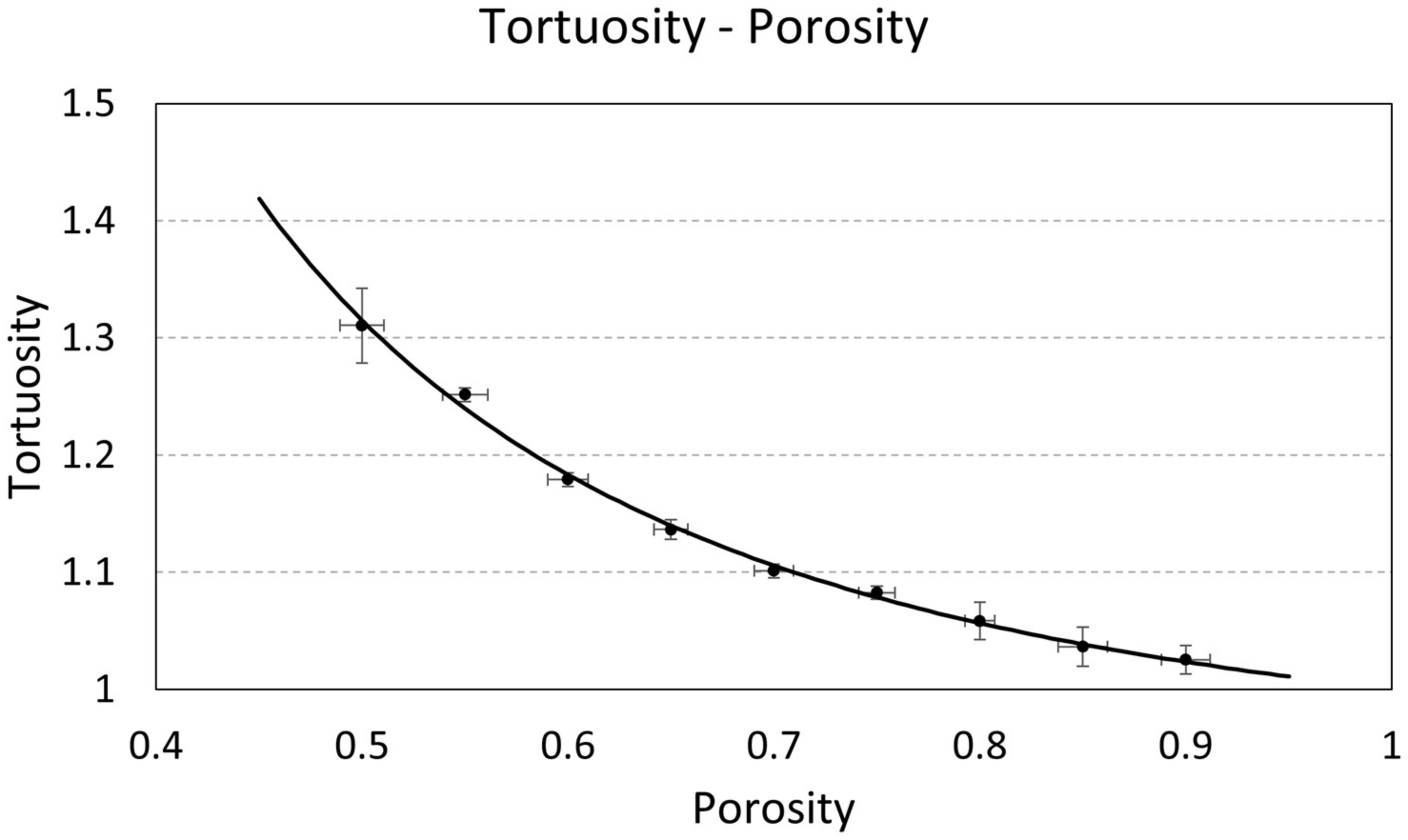
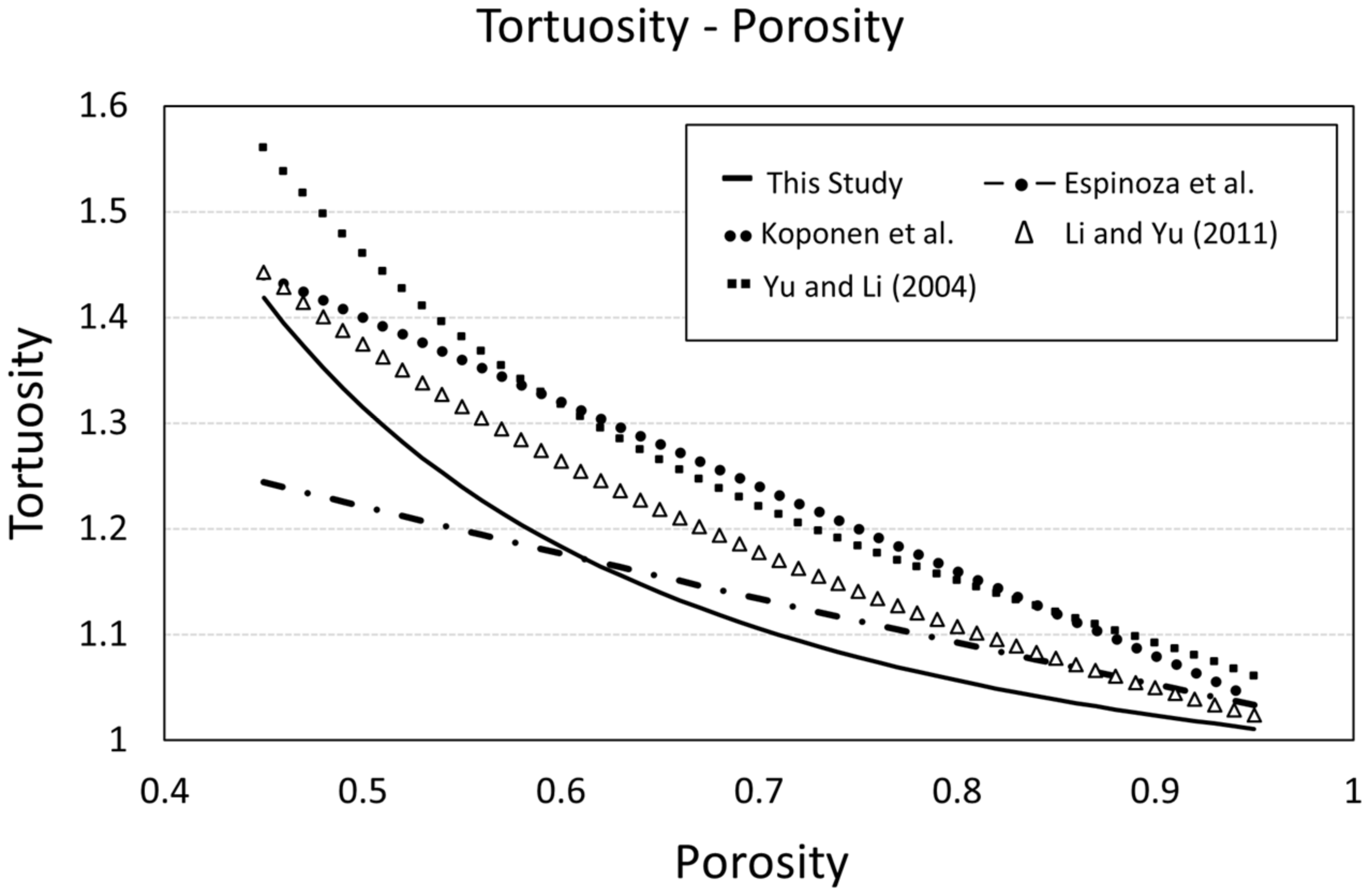
3.2. Tortuosity–Porosity Correlations

The corresponding curve fitting is applied to the data once the tortuosity values are computed for all the generated porous media. The three best correlations are selected and presented in Table 1. Given the aleatory characteristic of the porous media generation process, the tortuosities are computed for each sample group. The computed tortuosity values agree with the expected, i.e., lower values correspond to higher porosities, while higher values are related to lower porosities. The coefficient of determination is obtained directly from the MATLAB program and its value is used to select the best fitting curve; the higher the coefficient, the better the fitting.
Consequently, all selected correlations presented the behavior shown in previous studies, i.e., tortuosity behaves inversely proportional to porosity. Based on the results presented in Table 1, the correlation describing the geometric tortuosity behavior best is selected considering a high coefficient of determination. The power type is the correlation that best fits the obtained data, which also agrees with the widely known Brugemann correlation trend.
Figure 10 shows the obtained results that consider the range of porosity analyzed. It is crucial to notice that the proposed correlation describes the geometric tortuosity for porosities between 0.50 and 0.90. Figure 10 shows the selected correlation and the average values for each porosity and their corresponding deviation errors.
Table 2 is a collection of theoretical and empirical tortuosity–porosity correlations that satisfy the three requirements for tortuosity τ [40]. These are:
τ 2 = 1 ,
This means that the obtained path crossed by the species, while diffusing in the internal fluid in a porous domain, is greater than in the non-existence of the solid phase.
lim ϕ 1 τ = 1
That is, there is no diffusion in the absence of solid particles.
lim ϕ 0 τ   ;
i.e., the tortuosity is finite for all nonzero values of porosity.
The nature of the proposed correlation, i.e., the power type, complies with these conditions. Table 2 includes remarks on the physical system on which each correlation is based. These are useful to provide the validity of the obtained results, in contrast with other real-physical correlations.
Figure 11 depicts the proposed correlation obtained based on the current computational study and previously published results, considering the correlations presented in Table 2.
To compare the obtained results against other theoretical-empirical correlations, Figure 11 presents the tortuosity behavior of four tortuosity correlations as a function of porosity, considering two-dimensional porous media. As shown in Figure 11, for porosity values greater than 0.60, most of the correlations surpass the tortuosity values obtained in the current study. At the same time, for porosity values smaller than 0.60, the correlation presented by Espinoza et al. underestimates the tortuosity compared to the obtained values. At porosity values smaller than 0.50, the proposed correlation predicts similar tortuosity values to the presented by Koponen et al. [36] and Li and Yu [38]. Finally, the matching behavior of our correlation with the proposed, by Yu and Li [37] for the analyzed porosity range, is noted.

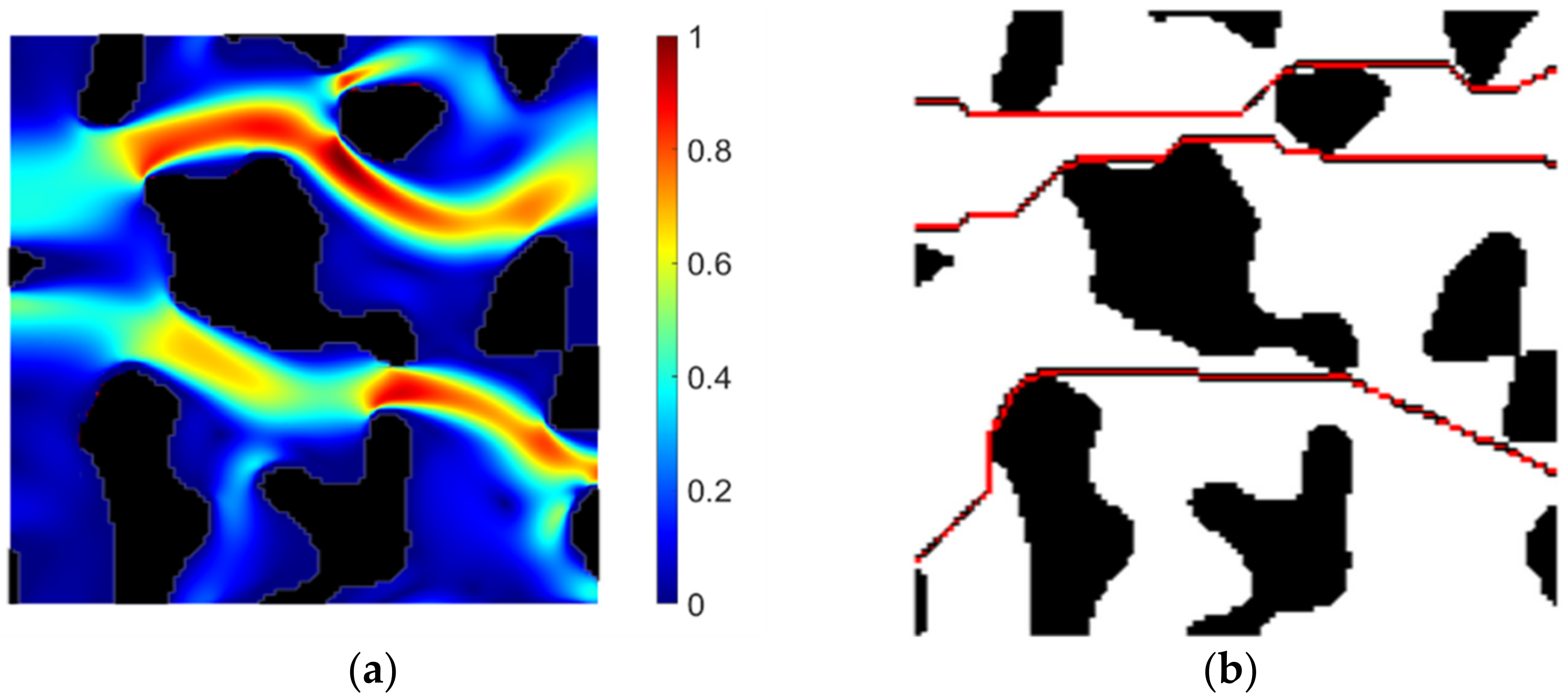
3.3. Hydraulic Tortuosity vs. Geometric Tortuosity

A comparison between the hydraulic and geometric tortuosity was performed. A digitally generated porous medium with a porosity of 0.75 was selected to analyze both tortuosity values.
First, the velocity field over the void spaces was computed following Equation (10). Then, the hydraulic tortuosity was determined. A MATLAB script simulating the lattice Boltzmann method was used to compute the hydraulic tortuosity. At the same time, the geometric tortuosity was calculated considering the A-star algorithm proposed in this study by using Equation (7). The results revealed that the hydraulic tortuosity was 𝜏 = 1.1768, and the geometric tortuosity computed using the A-star algorithm was 𝜏g = 1.1342. Thus, the geometric tortuosity is smaller than the hydraulic tortuosity by around 3.7%. Figure 12a shows the fluid’s velocity field through the selected porous domain, where the red regions are the spaces with higher velocities, while blue regions represent lower velocities. Figure 12b corresponds to the digital representation of the selected domain with some geometric paths obtained by the A-star algorithm to compare both the hydraulic and geometric tortuosity.

3.4. Geometric Tortuosity (A-Star) vs. Other Algorithms

Comparing the obtained results with previous studies, it was determined that when applying the skeleton shortest path method, a 10.685% deviation was found. That could happen, since the skeleton tends to consider more central paths into the pore space, in contrast to the A-star algorithm, whose paths can be closer to the obstacles or solid phase than to the center point of the pore phase. This can result in higher values, as shown in Table 3. Another algorithm considered, was the pore centroid. This procedure gave us an 8.503% deviation compared to our study. The reason can be similar since the pore centroid also estimates central points. Specifically, it considers centroids for path planning. This methodology can also result in higher values in contrast to the A-star algorithm. In the end, the Dijkstra algorithm was also computed and gave us a 3.655% deviation compared to our study. This was expected since the A-star algorithm has the Dijkstra procedure’s basis, however, with a heuristic function implemented.

4. Conclusions

An alternative method to compute several random porous media tortuosities with porosities between 0.50–0.90 was developed in this study. The porous media were digitally created with the help of the PoreSpy of Python library. These were combined with the pathfinding algorithm A-star to search the best paths and compute the geometric tortuosity. This method ensures an easy implementation to both study and test for further applications. The test was performed following valid statistical analyses in the scientific field.
On the other hand, this study was compared with previous studies and different algorithms to compute geometric tortuosity to guarantee the confidence of the values, obtaining satisfying results. Once the tortuosity was obtained, correlations were generated based on the calculated data. A total of 540 samples were randomly generated to allow for greater diversity in the study. The coefficient of determination metric was used to select the best predictive correlation. Hence, the best correlation based on the fitting parameters with a confidence interval of 95% is expressed with the power function. Finally, a possible step forward in this work is the consideration of three-dimensional porous media. In addition, the incidence of the geometric tortuosity of dead nodes, better defined as those nodes where a path ends without reaching an exit, will also be considered.

Author Contributions

Conceptualization, M.E.-A., J.P., J.Á. and J.B.-M.; data curation, M.E.-A., J.P. and J.Á.; formal analysis, M.E.-A., J.P. and J.Á.; funding acquisition, M.E.-A.; investigation, J.P. and J.Á.; methodology, M.E.-A., J.P., J.Á. and J.B.-M.; project administration, M.E.-A.; software, J.P. and J.Á.; supervision, M.E.-A. and J.B.-M.; validation, J.P., J.Á. and J.B.-M.; visualization, J.P. and J.Á.; writing—original draft, M.E.-A., J.P., J.Á. and J.B.-M.; writing—review and editing, M.E.-A. and J.B.-M. All authors have read and agreed to the published version of the manuscript.

Funding

This work has been funded by ESPOL through the grant number FIMCP-CERA-05-2017.

Institutional Review Board Statement

Not applicable.

Informed Consent Statement

Not applicable.

Data Availability Statement

The data presented in this study are available on request from the corresponding author. The data are not publicly available due to their current utilization for future works involving the authors of this paper.

Acknowledgments

The authors kindly acknowledge the support from ESPOL. Computational and physical resources provided by ESPOL are acknowledged. “Decanato de Investigación” support at ESPOL is also gratefully acknowledged.

Conflicts of Interest

The authors declare no conflict of interest.

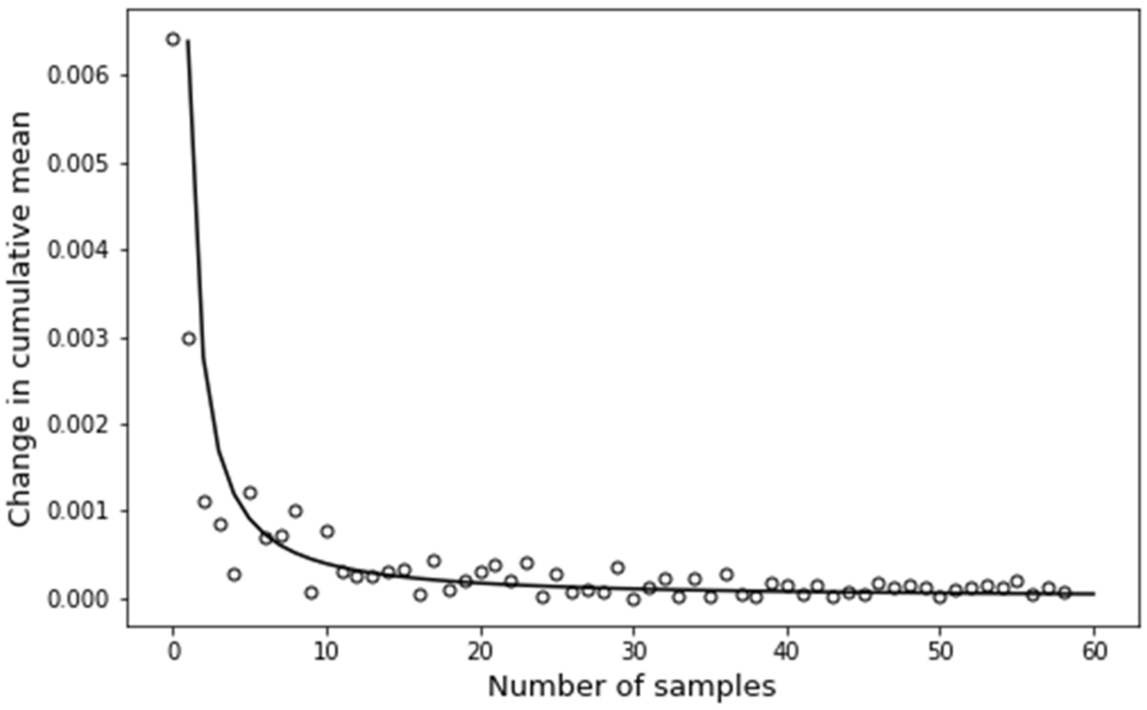
Appendix A. Determination of the Number of Samples

To determine the number of samples for each porosity value, a cumulative standard deviation (CSD) and standard error of the mean (SEM) analysis was performed [44]. Figure A1 and Figure A2 show that the CSD is stabilized around the sample numbers 40 to 50.
Furthermore, the CSD for the first 20 consecutive samples is smaller than 0.006 and 0.0004, and the average calculation of the coefficient of variation (CV) for all samples is around 0.45%.
Figure A1. CSD and SEM behavior of geometric tortuosity of calculated samples.
Computation 10 00059 g0a1
Figure A2. Evaluation of the cumulative mean shows a trend as the number of samples increases.
Computation 10 00059 g0a2
Based on all samples’ SEM obtained, the whole population falls between 1.24 and 1.26, with a 95% confidence level. In addition, the change in the cumulative average is shown in Figure A3.
Figure A3. Geometric tortuosity variation as the number of samples increases.
Computation 10 00059 g0a3
As observed, the cumulative average decreases as the number of samples increases. This result is expected compared to the law of large numbers (LLN) in experiments. The solid line shows how the cumulative mean behaves for one sample generated n times. The behavior can be represented with the following function:
f ( n ) = 0.006392     n 1.211
According to Equation (A1), when the number of samples is high, the difference in the consecutive values, i.e., actual and previous, of the cumulative mean tends to be zero.

References

  1. Fu, J.; Thomas, H.R.; Li, C. Tortuosity of porous media: Image analysis and physical simulation. Earth-Sci. Rev. 2021, 212, 1–52. [Google Scholar] [CrossRef]
  2. Valdés-Parada, F.J.; Porter, M.L.; Wood, B.D. The Role of Tortuosity in Upscaling. Transp. Porous Media 2011, 88, 1–30. [Google Scholar] [CrossRef]
  3. Friedman, S.P. Critical path analysis of the relationship between permeability and electrical conductivity of three-dimensional pore networks. Water Resour. Res. 1998, 34, 1703–1710. [Google Scholar] [CrossRef]
  4. Ghanbarian, B.; Hunt, A.G.; Ewing, R.P.; Sahimi, M. Tortuosity in Porous Media: A Critical Review. Soil Sci. Soc. Am. J. 2013, 77, 1461–1477. [Google Scholar] [CrossRef]
  5. Zhang, X.; Knackstedt, M.A. Direct simulation of electrical and hydraulic tortuosity in porous solids. Geophys. Res. Lett. 1995, 22, 2333–2336. [Google Scholar] [CrossRef]
  6. Encalada, Á.; Barzola-Monteses, J.; Espinoza-Andaluz, M. A Permeability–Throat Diameter Correlation for a Medium Generated with Delaunay Tessellation and Voronoi Algorithm. Transp. Porous Media 2020, 132, 201–217. [Google Scholar] [CrossRef]
  7. Ciurică, S.; Lopez-Sublet, M.; Loeys, B.L.; Radhouani, I.; Natarajan, N.; Vikkula, M.; Maas, A.H.E.M.; Adlam, D.; Persu, A. Arterial Tortuosity Novel Implications for an Old Phenotype. Australas. Phys. Eng. Sci. Med. 2019, 73, 951–960. [Google Scholar] [CrossRef]
  8. Espinoza-Andaluz, M.; Andersson, M.; Sundén, B. Computational time and domain size analysis of porous media flows using the lattice Boltzmann method. Comput. Math. Appl. 2017, 74, 26–34. [Google Scholar] [CrossRef]
  9. Encalada-Dávila, Á.; Espinoza-Andaluz, M.; Barzola-Monteses, J.; Li, S.; Andersson, M. Transport Parameter Correlations for Digitally Created PEFC Gas Diffusion Layers Using OpenPNM. Processes 2021, 9, 1141. [Google Scholar] [CrossRef]
  10. Delling, D.; Sanders, P.; Schultes, D.; Wagner, D. Engineering route planning algorithms. In Algorithmics of Large and Complex Networks; Springer: Berlin/Heidelberg, Germany, 2009; Volume 5515 LNCS, pp. 117–139. [Google Scholar] [CrossRef] [Green Version]
  11. Storandt, S. Contraction hierarchies on grid graphs. In Annual Conference on Artificial Intelligence; Springer: Berlin/Heidelberg, Germany, 2013; Volume 8077 LNAI, pp. 236–247. [Google Scholar] [CrossRef]
  12. Bast, H.; Funke, S.; Matijevic, D.; Sanders, P.; Schultes, D. In transit to constant time shortest-path queries in road networks. In Proceedings of the Ninth Workshop on Algorithm Engineering and Experiments (ALENEX), New Orleans, LA, USA, 6 January 2007; pp. 46–59. [Google Scholar] [CrossRef] [Green Version]
  13. Rios, L.H.O.; Chaimowicz, L. A survey and classification of A* based best-first heuristic search algorithms. In Brazilian Symposium on Artificial Intelligence; Springer: Berlin/Heidelberg, Germany, 2010; Volume 6404 LNAI, pp. 253–262. [Google Scholar] [CrossRef] [Green Version]
  14. Rusell, S.J.; Norvig, P. Artificial Intelligence: A Modern Approach, 3rd ed.; Davis, E., Edwards, D.D., Forsyth, D., Hay, N.J., Malik, J.M., Mittal, V., Sahami, M., Thrun, S., Eds.; Pearson Education: London, UK, 2010; ISBN 9780136042594. [Google Scholar]
  15. Stenzel, O.; Pecho, O.; Holzer, L.; Neumann, M.; Schmidt, V. Predicting Effective Conductivities Based on Geometric Microstructure Characteristics. AIChE J. 2016, 62, 1834–1843. [Google Scholar] [CrossRef]
  16. Shanti, N.O.; Chan, V.W.L.; Stock, S.R.; De Carlo, F.; Thornton, K.; Faber, K.T. X-ray micro-computed tomography and tortuosity calculations of percolating pore networks. Acta Mater. 2014, 71, 126–135. [Google Scholar] [CrossRef]
  17. Taiwo, O.O.; Finegan, D.P.; Eastwood, D.S.; Fife, J.L.; Brown, L.D.; Darr, J.A.; Lee, P.D.; Brett, D.J.L.; Shearing, P.R. Comparison of three-dimensional analysis and stereological techniques for quantifying lithium-ion battery electrode microstructures. J. Microsc. 2016, 263, 280–292. [Google Scholar] [CrossRef] [PubMed] [Green Version]
  18. Zharbossyn, A.; Berkinova, Z.; Boribayeva, A.; Yermukhambetova, A.; Golman, B. Analysis of tortuosity in compacts of ternary mixtures of spherical particles. Materials 2020, 13, 4487. [Google Scholar] [CrossRef] [PubMed]
  19. Tjaden, B.; Brett, D.J.L.; Shearing, P.R. Tortuosity in electrochemical devices: A review of calculation approaches. Int. Mater. Rev. 2018, 63, 47–67. [Google Scholar] [CrossRef] [Green Version]
  20. Lotito, V.; Zambelli, T. Pattern detection in colloidal assembly: A mosaic of analysis techniques. Adv. Colloid Interface Sci. 2020, 284, 102252. [Google Scholar] [CrossRef] [PubMed]
  21. Lotito, V.; Zambelli, T. A journey through the landscapes of small particles in binary colloidal assemblies: Unveiling structural transitions from isolated particles to clusters upon variation in composition. Nanomaterials 2019, 9, 921. [Google Scholar] [CrossRef] [Green Version]
  22. Lotito, V.; Zambelli, T. Playing with sizes and shapes of colloidal particles via dry etching methods. Adv. Colloid Interface Sci. 2022, 299, 102538. [Google Scholar] [CrossRef]
  23. Lotito, V.; Karlušić, M.; Jakšić, M.; Luketić, K.T.; Müller, U.; Zambelli, T.; Fazinić, S. Shape deformation in ion beam irradiated colloidal monolayers: An AFM investigation. Nanomaterials 2020, 10, 453. [Google Scholar] [CrossRef] [Green Version]
  24. Slotte, P.A.; Berg, C.F.; Khanamiri, H.H. Predicting Resistivity and Permeability of Porous Media Using Minkowski Functionals. Transp. Porous Media 2020, 131, 705–722. [Google Scholar] [CrossRef] [Green Version]
  25. Suzuki, A.; Miyazawa, M.; Okamoto, A.; Shimizu, H.; Obayashi, I.; Hiraoka, Y.; Tsuji, T.; Kang, P.K.; Ito, T. Inferring fracture forming processes by characterizing fracture network patterns with persistent homology. Comput. Geosci. 2020, 143, 104550. [Google Scholar] [CrossRef]
  26. Gostick, J.; Khan, Z.; Tranter, T.; Kok, M.; Agnaou, M.; Sadeghi, M.; Jervis, R. PoreSpy: A Python Toolkit for Quantitative Analysis of Porous Media Images. J. Open Source Softw. 2019, 4, 1296. [Google Scholar] [CrossRef]
  27. Wu, M.; Liu, J.; Lv, X.; Shi, D.; Zhu, Z. A Study on Homogenization Equations of Fractal Porous Media. J. Geophys. Eng. 2018, 15, 2388–2398. [Google Scholar] [CrossRef] [Green Version]
  28. Gunathilake, T.M.S.U.; Ching, Y.C.; Ching, K.Y.; Chuah, C.H.; Abdullah, L.C. Biomedical and microbiological applications of bio-based porous materials: A review. Polymers 2017, 9, 160. [Google Scholar] [CrossRef] [PubMed]
  29. Simaafrookhteh, S.; Shakeri, M.; Baniassadi, M.; Sahraei, A.A. Microstructure Reconstruction and Characterization of the Porous GDLs for PEMFC Based on Fibers Orientation Distribution. Fuel Cells 2018, 18, 160–172. [Google Scholar] [CrossRef]
  30. Espinoza, M.; Sunden, B.; Andersson, M.; Yuan, J. Analysis of Porosity and Tortuosity in a 2D Selected Region of Solid Oxide Fuel Cell Cathode Using the Lattice Boltzmann Method. ECS Trans. 2015, 65, 59–73. [Google Scholar] [CrossRef] [Green Version]
  31. Espinoza-Andaluz, M.; Velasco-Galarza, V.; Romero-Vera, A. On hydraulic tortuosity variations due to morphological considerations in 2D porous media by using the Lattice Boltzmann method. Math. Comput. Simul. 2020, 169, 74–87. [Google Scholar] [CrossRef]
  32. de Carvalho, T.P.; Morvan, H.P.; Hargreaves, D.M.; Oun, H.; Kennedy, A. Pore-Scale Numerical Investigation of Pressure Drop Behaviour Across Open-Cell Metal Foams. Transp. Porous Media 2017, 117, 311–336. [Google Scholar] [CrossRef] [Green Version]
  33. Grigoriev, M.; Khafizov, A.; Kokhan, V.; Asadchikov, V. Robust technique for representative volume element identification in noisy microtomography images of porous materials based on pores morphology and their spatial distribution. In Proceedings of the Thirteenth International Conference on Machine Vision. International Society for Optics and Photonics, Rome, Italy, 2–6 November 2020. [Google Scholar] [CrossRef]
  34. Ezzatabadipour, M.; Zahedi, H. A Novel Method for Streamline-Based Tortuosity Calculation and Investigation of Obstacles Shape Effect on Tortuosity in Porous Media with Random Elliptical Obstacles Using Lattice Boltzmann Method. Transp. Porous Media 2021, 136, 103–124. [Google Scholar] [CrossRef]
  35. Ferguson, D.; Likhachev, M.; Stentz, A. A guide to heuristic-based path planning. In Proceedings of the International Workshop on Planning under Uncertainty for Autonomous Systems, International Conference on Automated Planning and Scheduling (ICAPS), Monterey, CA, USA, 5–10 June 2005; pp. 1–10. [Google Scholar]
  36. Liu, C.; Mao, Q.; Chu, X.; Xie, S. An Improved A-star algorithm considering water current, traffic separation and berthing for vessel path planning. Appl. Sci. 2019, 9, 1057. [Google Scholar] [CrossRef] [Green Version]
  37. Espinoza, M.; Sundén, B.; Andersson, M. Pore-Scale Analysis of Diffusion Transport Parameters in Digitally Reconstructed SOFC Anodes with Gradient Porosity in the Main Flow Direction. ECS Trans. 2017, 78, 2785–2796. [Google Scholar] [CrossRef] [Green Version]
  38. Mohamad, A.A. Lattice Boltzmann Method, 2nd ed.; Springer: London, UK, 2019; ISBN 978-1-4471-7422-6. [Google Scholar]
  39. Cooper, S.J.; Kishimoto, M.; Tariq, F.; Bradley, R.S.; Marquis, A.J.; Brandon, N.P.; Kilner, J.A.; Shearing, P.R. Microstructural Analysis of an LSCF Cathode Using In Situ Tomography and Simulation. ECS Trans. 2013, 57, 2671–2678. [Google Scholar] [CrossRef]
  40. Shen, L.; Chen, Z. Critical review of the impact of tortuosity on diffusion. Chem. Eng. Sci. 2007, 62, 3748–3755. [Google Scholar] [CrossRef]
  41. Koponen, A.; Kataja, M.; Timonen, J. Tortuous flow in porous media. Phys. Rev. E Stat. Phys. Plasmas Fluids Relat. Interdiscip. Top. 1996, 54, 406–410. [Google Scholar] [CrossRef] [PubMed]
  42. Yu, B.M.; Li, J.H. A geometry model for tortuosity of flow path in porous media. Chin. Phys. Lett. 2004, 21, 1569–1571. [Google Scholar] [CrossRef]
  43. Li, J.H.; Yu, B.M. Tortuosity of flow paths through a Sierpinski carpet. Chin. Phys. Lett. 2011, 28, 3–6. [Google Scholar] [CrossRef]
  44. Ritter, F.E.; Schoelles, M.J.; Quigley, K.S.; Klein, L.C. Determining the Number of Simulation Runs: Treating Simulations as Theories by Not Sampling Their Behavior. In Human-in-the-Loop Simulations Methods Pract; Springer: London, UK, 2011; pp. 97–116. [Google Scholar]
Figure 1. Two-dimensional numerical representation of porous media for tortuosity explanation.
Computation 10 00059 g001
Figure 2. Comparison between two porous media with porosity of 0.5 and blobbiness of (a) 0.5 and (b) 1.0.
Computation 10 00059 g002
Figure 3. Flowchart of the porous media generation process.
Computation 10 00059 g003
Figure 4. Flowchart showing the steps for the porous media selection.
Computation 10 00059 g004
Figure 5. Schematic of a simplified porous medium showing roads with their possible arrival nodes.
Computation 10 00059 g005
Figure 6. The solid-void distribution and a path generated by the A-star algorithm in a simplified selected porous medium.
Computation 10 00059 g006
Figure 7. Possible directions followed during the application of the A-star algorithm in a two-dimensional grid.
Computation 10 00059 g007
Figure 8. Visual comparison between geometric (a) and hydraulic (b) paths in the same porous medium. White regions represent void spaces, while black regions represent solid materials. The fluid can pass only through the white regions, and the solid obstacles are considered impermeable. Lg represents the actual geometric path, while Lh corresponds to the actual hydraulic path.
Computation 10 00059 g008
Figure 9. Selected samples of generated porous media with porosity values of (a) 0.50, (b) 0.65, (c) 0.80, and (d) 0.90.
Computation 10 00059 g009
Figure 10. Tortuosity values trend as a function of the porosity represented by the power correlation from Table 2.
Computation 10 00059 g010
Figure 11. Comparison of tortuosity values obtained in the current study and others found in the literature.
Computation 10 00059 g011
Figure 12. Selected porous media in which the hydraulic and geometric tortuosity have been computed for their corresponding comparison. (a) Velocity field in the selected porous domain; color bar with normalized velocity values; and (b) geometric paths for the digital representation of the generated porous domain.
Computation 10 00059 g012
Table 1. Empirical tortuosity–porosity correlations for the generated porous media. The coefficient of determination for each possible correlation is also presented.
Empirical Correlation for τCoefficient of DeterminationType
9.112 · 10 2 · ϕ 2.155 + 0.9093   0.9975Power
3.524 · e 4.664 ϕ + 0.9703 0.9969Exponential
1.142 · ϕ 2 2.328 · ϕ + 2.187 0.9888Polynomial
Table 2. Theoretical and empirical tortuosity-porosity correlations available in the literature.
Correlation for τStructure A u t h o r Reference
0.8 ( 1 ϕ ) + 1 Randomly placed fully overlapping rectanglesKoponen et al. (1996) [41]
1 2 [ 1 + 1 2 1 ϕ + ( 1 1 ϕ ) 2 + 1 ϕ 4 1 1 ϕ ] Square shaped particlesYu and Li (2004) [42]
19 18 ln ( ϕ ) ln ( 8 9 ) Sierpinski carpetLi and Yu (2011) [43]
1.47 e 0.3708 ϕ Circle-shaped particlesEspinoza et al. (2019) [31]
Table 3. Comparison between other geometric tortuosity algorithms with our study.
Pathfinding MethodsTortuosity τRelative Deviation (%)
This study1.2747-
Pore centroid1.38318.503
Skeleton (PoreSpy)1.410910.685
Dijkstra1.32133.655
Publisher’s Note: MDPI stays neutral with regard to jurisdictional claims in published maps and institutional affiliations.

