Aggregating Composite Indicators through the Geometric Mean: A Penalization Approach

Abstract

In this paper, we introduce a penalized version of the geometric mean. In analogy with the Mazziotta Pareto Index, this composite indicator is derived as a product between the geometric mean and a penalization term to account for the unbalance among indicators. The unbalance is measured in terms of the (horizontal) variability of the normalized indicators opportunely scaled and transformed via the Box–Cox function of order zero. The penalized geometric mean is used to compute the penalized Human Development Index (HDI), and a comparison with the geometric mean approach is presented. Data come from the Human Development Data Center for 2019 and refer to the classical three dimensions of HDI. The results show that the new method does not upset the original ranking produced by the HDI but it impacts more on countries with poor performances. The paper has the merit of proposing a new reading of the Mazziotta Pareto Index in terms of the reliability of the arithmetic mean as well as of generalizing this reading to the geometric mean approach.

1. Introduction

In recent years, there is an increasing interest in well-being measurement through composite indicators which are obtained combining individual indicators into a single index, based on an underlying model of the multidimensional concept that is being measured [1]. In the debate about composite indicators, the choice of the aggregation method is the core issue. Indeed, each aggregation method has a corresponding aggregation function, namely the transformation of the indicators used to obtain the composite indicator. Usually, there are two criteria used for choosing among different aggregation functions. The first is related to the importance of the single indicator and the second addresses the issue of compensability or substitutability among indicators. The importance of an indicator is measured by the marginal contribution of the indicator computed as the partial derivative of the aggregation function with respect to the indicator, when the aggregation function is differentiable. The compensability refers to the possibility of offsetting the low value of an indicator with a high value of another indicator.

This paper addresses the problem of indicator aggregation through a non-compensative approach by means of a penalization factor that captures the unbalance among indicators. The aim of the paper is twofold. Firstly, in line with the interpretation of arithmetic mean as a least-squares estimate for the data values transformed by the Box–Cox function of order one as in Berger and Casella [2], we propose a new reading of the so-called Mazziotta and Pareto Index (hereafter, MPI) [3] in terms of the Box–Cox transformation of order one. Secondly, we propose a generalization of the formula obtained for the MPI to obtain a penalized version of the geometric mean. Specifically, the penalized geometric mean is obtained as the product between the geometric mean and a penalization factor that depends on the (horizontal) variance of the normalized indicators opportunely scaled and transformed via the Box–Cox function of order zero. Roughly speaking, the penalization factor is a correction term to the geometric mean, which accounts for the unbalance among indicators. In fact, under the Box Cox transformation, the penalization factor is the variance of the scaled normalized indicators obtained by dividing the normalized indicators by their geometric mean. This is the reason why the penalization factor can be interpreted as a reliability measure for the geometric mean. Hence, the higher the unbalance among indicators, the higher the penalization.

The method presented here to penalize the geometric mean can be easily applied to every generalized means considering the appropriate Box–Cox transformation. In this paper, we make a first attempt to bridge two strands of the scientific literature concerning the use of generalized means as aggregation operators, that is: the composite indicator construction and the information theory [4].

To illustrate the appealing of our proposal, we focus on the construction of the Human Development Index (HDI). The index emerged in the first Human Development Report (HDR), which was published by the United Nations Development Programe in 1990. (All editions are available at: https://hdr.undp.org/en/global-reports, accessed on 28 February 2022.) The index is computed annually for more than 170 countries by combining three dimensions: longevity, knowledge, and access to resources. The longevity aspect is captured by life expectancy at birth. The knowledge pillar is represented by a measure of educational achievement, which is measured as a weighted sum of expected year of schooling (adult literacy) and of mean year of schooling. Finally, the resource dimension is represented by an adjusted real purchasing power parity: GDP per capita.

The paper is organized as follows: in Section 2, we discuss the problem of compensation and balance among indicators and we review the relevant literature. In Section 3, we propose a new reading for the Mazziotta Pareto Index. In Section 4, we introduce the penalized geometric mean and we present the theoretical framework. In Section 5, we apply the penalized geometric mean to compute the “penalized” Human Development Index (pHDI) and we compare HDI with pHDI in terms of the corresponding rankings. Section 6 concludes and suggests possible extensions. Proofs of some propositions of Section 4 are collected in the Appendix A.

2. Literature Review

2.1. Compensability and Balance among Indicator

The simplest aggregation approach makes use of the arithmetic mean. Despite its ease of interpretation, the arithmetic mean suffers from two main drawbacks: the fully compensability or perfect substitutability and the (possible low) reliability. The perfect substitutability allows for unbalances among indicators without considering any penalization for the unbalance. This means that different distributions of indicator values can yield similar or equal value of the composite indicator. Therefore, the unbalance gives rise to a loss of information about the multidimensional nature of the phenomenon under investigation. In this sense, the fully compensability and the unbalance have negative effects on the composite indicator and, for this reason, deserve consideration. On the other hand, it should be recalled that the arithmetic mean is a central tendency measure whose reliability depends strongly on the dispersion of the data around it. Usually, when the sample size is large enough, the dispersion is measured in terms of the standard deviation of data from the mean. The smaller/larger the standard deviation, the larger/smaller the mean value reliability. In the context of composite indicators, the dispersion to be considered is the horizontal dispersion—that is, the dispersion measured across indicators—to distinguish from the vertical dispersion—that is, the dispersion across units.

The next paragraphs will be devoted to review the main aspects of compensability and balance among indicators and to provide a summary of the methods used for computing HDI.

When the computation of a composite indicator is based on a linear (weighted) aggregation rule, full compensability among the individual indicators is always assumed. This implies that there is substitutability among the different aspects and, consequently, poor performance in one aspect can be completely compensated by surplus in another one. However, for a hypothetical well-being indicator, could life expectancy be compensated by income? Thus, a complete compensability among indicators is often not desirable.

The literature accounts for several non-compensative approaches. For instance, to rank countries, when we use as a composite index the minimum value among the (normalized) indicators, any improvements in the other indicators cannot modify the value of the final index. However, this approach is not without drawbacks, since it does not consider the unbalance among indicators. Moreover, two countries with very different profiles but with a common minimum will display the same value of the index and ranked at the same position.

Among the non-compensative approaches, the family of aggregation functions based on generalized means of power $\alpha ,$ $\alpha \in \mathbb{R},$ plays a crucial role. For example, the geometric mean $(\alpha =0)$ is used to compute the Human Development Index [5], whereas the Human Poverty Index for developing countries (HPI-1) computed by UNDP [6] is obtained using the generalized mean of power $\alpha =3.$

The non-compensative aggregation methods, as like the generalized means, overcome only partially the drawbacks of the arithmetic mean approach, penalizing the unbalance among indicators. Specifically, in the geometric mean approach, the marginal increase in the value of an indicator is much higher when the absolute value of the indicator is low. In this way, the performance of the high indicators is penalized, and the improvements in the weak indicators are encouraged. However, it should be noted that the penalization introduced by the geometric mean considers only partially the unbalance issue. The following example could clarify the point. Let us consider a composite indicator obtained as the geometric mean of two indicators whose normalized values range between $e^0$ and $e^1.$ The normalized values $z_1=e^0$ and $z_2=e^1$ yield the same composite indicator value $e^{0.5}$ that would be obtained with $z_1=z_2=e^{0.5}.$ Therefore, despite its non-compensative nature, the geometric mean approach attributes the same value of composite indicator to two pairs of indicator values that have very different distributions and horizontal dispersions.

In particular, we note that the use of the geometric mean is not decisive to fully balance the contributions of the single indicators. The reason for this weakness is that the geometric mean is strongly related to the arithmetic mean via Box–Cox transformation of order zero [7]. In fact, if we take the arithmetic mean of the logarithm of the indicator values, we get the same as if we take the logarithm of their geometric mean. Thereby, in the transformed space, the geometric mean suffers from the same drawbacks of the arithmetic mean.

A first attempt to consider the unbalance among indicators is made by Casadio Tarabusi and Palazzi [8] that uses the concave average approach to build the aggregation function of the Sustainability Development Index. This function is obtained as the weighted average of a strictly concave parametric transformation of the normalized indicators, whose parameters adjust the intensity of the unbalance penalization. More recently, Casadio Tarabusi and Guarini [9] combine non-linearly the weighted arithmetic mean and the Min function in a parametric aggregation function, called Mean-Min function, with the purpose of mediating the minimum penalization (represented by the arithmetic mean) and the maximum penalization (represented by the Min function). Moreover, the authors introduce a measure of compensation between a couple of indicators, called Marginal Rate of Compensation (MRC), in order to evaluate the proportion of marginal increase (decrease) of an indicator compensated by a marginal decrease (increase) of another indicator (keeping the remaining variables unchanged).

In the scientific literature, many other non-compensatory aggregation methods are suggested. According to El Gibari et al. [10], the construction of a composite indicator involves multi-criteria decision-making (MCDM) theory. They classify the different MCDM methods in five different categories: (i) elementary methods; (ii) value and utility-based methods; (iii) data envelopment analysis-based methods; (iv) distance functions-based methods; and (v) the outranking relation approach. In the first category, the Simple Additive Weighting (SAW) and the Weighted Product (WP) imply a total compensation in the case of the SAW method and a partial compensation in the case of the WP method. According to Lai et al. [11], the main advantage of those methods is that they can reduce complex problems by simple conditions. The second category refers to methods that assign a real number to each alternative and determine a preference order for the alternatives based on decision-makers’ value judgements [12]. The Data Envelopment Analysis (DEA)-based methods use a linear programming as instrumental variable to evaluate the efficiency of a set of comparable units. DEA allows for full compensation among the criteria [13]. The distance function method requires the definition of a reference point and a function that measures the deviation between the values of each indicator and their corresponding reference levels [14]. Finally, the outranking relation approach demands a comparison between pairs of options to compare alternatives, in order to state if a given alternative is at least as good as another one. According to El Gibari et al. [10], the two most used methods in this last category are the ELECTRE (Elimination and Choice Expressing Reality [15]) and PROMETHEE (Preference Ranking Organization Method for Enrichment Evaluations [16]). Greco et al. [17] identify these two methods as the two main types of non-compensatory aggregation techniques.

The literature includes also the so-called Mixed Strategies. The name derives from the fact that it cannot fit into one category or another, since they use a combination of different approaches for solving the aforementioned issues [17]. This is the case of the Mazziotta Pareto method [18].

The Mazziotta Pareto Index (MPI) derives from the Method of Penalties by Coefficient of Variation proposed by the same authors to measure the health infrastructure endowment under the assumption of non-substitutability of the indicators. The MPI uses as aggregation function the arithmetic mean adjusted by a penalization coefficient that accounts for the (horizontal) variability of (opportunely standardized) indicators in relation to the mean, with the purpose of penalizing the unbalanced distribution of the indicators.

A newer variant of the index allows for comparisons over time [19]. The Adjusted MPI (AMPI) method uses a different normalization procedure from a modified $z$-score to a rescaling method. In addition, it allows for choosing reference points, the so-called goalposts, e.g., to fix to 100 the average in a given year to facilitate the interpretation of results.

2.2. The Human Development Index

To illustrate the proposed method, we focus on one of the most famous composite indicators defined by means of a geometric mean, namely the Human Development Index, and we compute its corresponding penalized version.

In the original formulation, the HDI was computed as the arithmetic mean of the three dimensions: life expectancy, education, and GDP per capita. In 2010, the arithmetic mean has been replaced by the geometric mean [5]. There are at least two advantages in the use of the geometric mean instead of the arithmetic mean. Firstly, the geometric mean reduces the level of substitutability between dimensions. Secondly, the geometric mean ensures that a 1% decline in one dimension has the same impact on the aggregate index as a 1% decline in another dimension. Over the years, many modifications of the geometric mean approach have been proposed. For instance, Noorbakhsh [20] proposes to modify the normalization process. Paul [21] suggests to overcome what he defines as the problem of underestimation of achievement at the higher level by assigning higher weights to each of the physical indicators at the margin. Others scholars have proposed to modify the indicators; for instance, Jha et al. [22] propose to modify the health dimension to account for a morbidity situation, and Prados de la Escosura [23] suggests to modify the non-income dimensions by applying a convex achievement function. The HDI has also been investigated from a theoretical point of view. For instance, Chakravarty [24] axiomatically characterizes a family of measures of achievement that reduces to HDI as a special case. Finally, Alkire and Forster [25] propose a multiplicative modification of the HDI that accounts for the inequality by introducing a multiplicative inequality measure based on the Atkinson inequality family.

3. A New Reading of the Mazziotta Pareto Index

According to the Method of Penalties by Coefficient of Variation [18,26] denoting by $x_{ij}$ the value of the indicator j relative to the i-th unit, $i=1,2,\dots ,n,$ $j=1,2,\dots ,m,$ the normalized value of the indicator j relative to the i-th unit is obtained standardizing $x_{ij}$ to have a mean of 100 and standard deviation of 10, as follows:

$$\begin{array}{c}\hfill z_{ij}=100\pm \frac{x_{ij}-M_{x_j}}{S_{x_j}}10,i=1,2,\dots ,n,j=1,2,\dots ,m,\end{array}$$

(1)

where $M_{x_j}$ and $S_{x_j}$ are, respectively, the mean and the standard deviation of the j-th indicator. Starting from the normalized indicators (1), the MPI relative to the i-th unit is defined as:

$$\begin{array}{c}\hfill MP{I}_i^{\pm }={\mu }_i\left(1\pm \frac{S_i^2}{{\mu }_i^2}\right),i=1,2,\dots ,n,\end{array}$$

(2)

where

$$\begin{array}{c}\hfill {\mu }_i=\frac{1}{m}\sum _{j=1}^m{z}_{ij},i=1,2,\dots ,n,\end{array}$$

(3)

is the arithmetic mean of the normalized indicators for unit i, and

$$\begin{array}{c}\hfill S_i^2=\frac{1}{m}\sum _{j=1}^m{(z_{ij}-{\mu }_i)}^2,i=1,2,\dots ,n,\end{array}$$

(4)

is the (biased) sample variance of the normalized indicators $z_{ij}$ for unit $i,$ $i=1,2,\dots ,n.$ The term $1\pm S_i^2/{\mu }_i$ in (2) penalizes the arithmetic mean ${\mu }_i$ to account for the (horizontal) variability of the normalized indicators. The addition of this penalization has two main effects: firstly, it makes the MPI not fully compensable; secondly, it discriminates between units with the same arithmetic mean using a criterion that deals with the reliability of the arithmetic mean itself. In fact, the MPI penalizes more the units with larger (horizontal) variability and, as a consequence, with smaller arithmetic mean reliability. We recall that the ± sign in (2) depends on the type of phenomenon considered; if increasing variations of the indicator correspond to positive variations of the phenomenon (positive polarity), we choose the sign $-$, otherwise (negative polarity), we choose the sign $+$.

We propose a new reading of the Mazziotta Pareto Index, with the twofold purpose of interpreting the penalization term in (2) as a measure of the error committed using the arithmetic mean instead of the normalized indicators, and of extending this idea to generalized means. In this paper, we focus on the geometric mean, but the generalization proposed here can be applied to all the other generalized means and it will be surely an object of further research.

In order to understand the new reading of the Mazziotta Pareto Index, it is necessary to introduce the interpretation of the arithmetic mean proposed by Berger and Casella [2], according to which the generalized means can be derived as least square estimates of data transformed via a Box–Cox function [7] Specifically, according to Berger and Casella, the arithmetic mean ${\mu }_i$ in (14) can be read as the solution of the following optimization problem:

$$\begin{array}{c}\hfill \underset{a\in \mathbb{R}}{min}F\left(a\right),\end{array}$$

(5)

where

$$\begin{array}{c}\hfill F\left(a\right)=\frac{1}{m}\sum _{j=1}^m{(h_1\left(z_{ij}\right)-h_1\left(a\right))}^2,a\in \mathbb{R},\end{array}$$

(6)

and $h_1\left(x\right)$ is the Box–Cox transformation of order one defined as:

$$\begin{array}{c}\hfill h_1\left(x\right)=x-1,x\in \mathbb{R}.\end{array}$$

(7)

That is, ${\mu }_i,$ as a solution of (5), is the preimage under $h_1$ of the least squares estimate of the normalized indicators transformed via the function $h_1,$ i.e.,

$$\begin{array}{c}\hfill {\mu }_i=h_1^{-1}\left(\frac{1}{m}\sum _{j=1}^m{h}_1\left(z_{ij}\right)\right),i=1,2,\dots ,n.\end{array}$$

(8)

Under the Box–Cox transformation $h_1$, the error made approximating the normalized indicators relative to the $i$-th unit with ${\mu }_i$ is the value of function (6) at the optimum ${\mu }_i$, and it coincides with the (biased) sample variance of $z_{ij}$, $j=1,2,\dots ,m,$ i.e.,

$$\begin{array}{c}\hfill F\left({\mu }_i\right)=\frac{1}{m}\sum _{j=1}^m{(h_1\left(z_{ij}\right)-h_1\left({\mu }_i\right))}^2=\frac{1}{m}\sum _{j=1}^m{(z_{ij}-{\mu }_i)}^2=S_i^2,i=1,2,\dots ,n.\end{array}$$

(9)

The reliability of ${\mu }_i$ depends on the size of (9). It should be pointed out that every unit $i$, $i=1,2,\dots ,n,$ has a corresponding error $S_i^2$ whose size depends strongly on ${\mu }_i.$ Thereby, the errors relative to units with different means are not comparable.

In order to overcome this difficulty, we consider the scaled normalized indicators obtained dividing the normalized indicators relative to the i-th unit by the corresponding arithmetic mean ${\mu }_i,$ i.e.,

$$\begin{array}{c}\hfill {\tilde{z}}_{ij}=\frac{z_{ij}}{{\mu }_i},i=1,2,\dots ,n.\end{array}$$

(10)

It is simple to see that the arithmetic mean, ${\tilde{\mu }}_i,$ of the scaled values ${\tilde{z}}_{ij}$, $j=1,2,\dots ,m,$ is equal to one for every unit $i$, $i=1,2,\dots ,n.$ Under the Box–Cox transformation $h_1,$ the error made approximating the scaled normalized indicators ${\tilde{z}}_{ij}$ relative to the i-th unit with ${\tilde{\mu }}_i=1$ is:

$$\begin{array}{c}\hfill {\tilde{S}}_i^2=\frac{1}{m}\sum _{j=1}^m{h}_1{\left({\tilde{z}}_{ij}\right)}^2=\frac{1}{m}\sum _{j=1}^m{h}_1{\left(\frac{z_{ij}}{{\mu }_i}\right)}^2,i=1,2,\dots ,n.\end{array}$$

(11)

The error in (11) coincides with the (biased) sample variance of the scaled normalized indicators ${\tilde{z}}_{ij}$ transformed via the function $h_1.$ Note that (11) is independent from the size of ${\tilde{\mu }}_i$ (that is the same for each unit) and allows for a comparison between units with different means. The higher the value of ${\tilde{S}}_i^2,$ the higher the loss of information caused by considering ${\mu }_i$ instead of the normalized indicators $z_{ij},$ no matter the value of ${\mu }_i.$

Note that:

$$\begin{array}{c}\hfill {\tilde{S}}_i^2=\frac{S_i^2}{{\mu }_i^2},i=1,2,\dots ,n,\end{array}$$

(12)

is the squared coefficient of variation of $z_{ij}$, $j=1,2,\dots ,m.$ Moreover, the MPI relative to the i-th unit defined in (2) can be rewritten as follows:

$$\begin{array}{c}\hfill MP{I}_i^{\pm }={\mu }_i{h}_1^{-1}(\pm {\tilde{S}}_i^2),i=1,2,\dots ,n.\end{array}$$

(13)

Equation (13) proposes a new reading of the penalization term appearing in the MPI Formula (2), according to which the penalization term is nothing more than the preimage under $h_1$ of $\pm {\tilde{S}}_i^2$. The larger the error ${\tilde{S}}_i^2$ (and, as a consequence, smaller the reliability of ${\mu }_i$), the smaller (in the case of positive polarity) or larger (in the case of negative polarity) the value of MPI. Therefore, the idea is to discriminate between units with the same arithmetic mean but different arithmetic mean reliability, attributing smaller (in the case of positive polarity) or larger (in the case of negative polarity) MPI value to the units for which the arithmetic mean is less reliable.

4. The Penalized Geometric Mean

According to the interpretation of Berger and Casella illustrated in the previous section, the composite indicator relative to the $i$-th unit given by the geometric mean of the normalized indicators $z_{ij}$:

$$\begin{array}{c}\hfill {\displaystyle {\mu }_{0,i}={\left(\prod _{j=1}^m{z}_{ij}\right)}^{\frac{1}{m}},i=1,2,\dots ,n,}\end{array}$$

(14)

can be expressed as a preimage of the least squares estimate of the normalized indicators transformed via the Box–Cox function of order zero, $h_0,$ as follows:

$$\begin{array}{c}\hfill {\mu }_{0,i}=h_0^{-1}\left(\frac{1}{m}\sum _{j=1}^m{h}_0\left(z_{ij}\right)\right),i=1,2,\dots ,n,\end{array}$$

(15)

where $h_0$ is defined as:

$$\begin{array}{c}\hfill h_0\left(x\right)=lnx,x\in {\mathbb{R}}_{+}.\end{array}$$

(16)

In analogy with the interpretation of MPI in Section 3, we define the penalized geometric mean as follows:

$$\begin{array}{c}\hfill G{M}_i^{\pm }={\mu }_{0,i}{h}_0^{-1}\left(\pm {\tilde{S}}_{0,i}^2\right)={\mu }_{0,i}exp\{\pm {\tilde{S}}_{0,i}^2\},i=1,2,\dots ,n,\end{array}$$

(17)

where

$$\begin{array}{c}\hfill {\tilde{S}}_{0,i}^2=\frac{1}{m}\sum _{j=1}^m{h}_0{\left(\frac{z_{ij}}{{\mu }_{0,i}}\right)}^2=\frac{1}{m}\sum _{j=1}^m{\left(ln{z}_{ij}-ln{\mu }_{0,i}\right)}^2,i=1,2,\dots ,n,\end{array}$$

(18)

is the (biased) sample variance of the scaled normalized indicators ${\widehat{z}}_{ij}=z_{ij}/{\mu }_{0,i},$ $j=1,2,\dots ,m,$ transformed via the function $h_0.$

The penalized geometric mean (17) is obtained multiplying the geometric mean ${\mu }_{0,i}$ with the penalization factor $h_0^{-1}(\pm {\tilde{S}}_{0,i}^2)$ with the purpose of discriminating between units with same geometric mean but different geometric mean reliability, attributing smaller (in the case of positive polarity) or larger (in the case of negative polarity) value to the units for which the geometric mean is less reliable. Analogously to the MPI, the reliability of the geometric mean ${\mu }_{0,i}$ is measured in terms of the reliability of the arithmetic mean of $h_0\left({\widehat{z}}_{ij}\right),$ $j=1,2,\dots ,m.$

Proposition 1.

The penalized geometric mean (17) satisfies the following properties:

1.

$G{M}_i^{+}\ge {\mu }_{0,i}\ge G{M}_i^{-}$.

2.

$G{M}_i^{+}=G{M}_i^{-}={\mu }_{0,i},ifandonlyif{\tilde{S}}_{0,i}=0$.

3.

$G{M}_i^{+}=G{M}_i^{-}exp\left\{2{\tilde{S}}_{0,i}^2\right\}$.

4.

Given two units k and h ($k\ne h$) with ${\mu }_{p,k}={\mu }_{p,h},$ we have:

$$\begin{array}{cc}\hfill G{M}_k^{-}>G{M}_h^{-}& iff{\tilde{S}}_{0,h}^2>{\tilde{S}}_{0,k}^2,\hfill \\ \hfill G{M}_k^{+}>G{M}_h^{+}& iff{\tilde{S}}_{0,k}^2>{\tilde{S}}_{0,h}^2.\hfill \end{array}$$

5.

Given two units k and h ($k\ne h$) we have:

$$\begin{array}{cc}\hfill G{M}_k^{-}>G{M}_h^{-}& iff{\mu }_{0,k}>{\mu }_{0,h}exp\left\{{\tilde{S}}_{0,k}^2-{\tilde{S}}_{0,h}^2\right\},\hfill \\ \hfill G{M}_k^{+}>G{M}_h^{+}& iff{\mu }_{0,k}>{\mu }_{0,h}exp\left\{{\tilde{S}}_{0,h}^2-{\tilde{S}}_{0,k}^2\right\}.\hfill \end{array}$$

Proof. 

The proof follows easily from (8). □

The following propositions list some properties of $G{M}_i^{\pm }$ as a function of $z_{ik}$, $i=1,2,\dots ,n$ and $k=1,2,\dots ,m.$

Proposition 2.

For $i=1,2,\dots ,n$ and $k=1,2,\dots ,m$ the penalized geometric mean (17) satisfies the following properties:

1.

${\displaystyle \frac{\partial G{M}_i^{-}}{\partial z_{ik}}\ge 0}$ for $z_{ik}\le z_i^{-}$ and has a local maximum at the point $z_i^{-},$

2.

${\displaystyle \frac{\partial G{M}_i^{+}}{\partial z_{ik}}\ge 0}$ for $z_{ik}\ge z_i^{+}$ and has a local minimum at the point $z_i^{+},$

where ${\displaystyle z_i^{\pm }={\mu }_{0,i}exp\left\{\mp \frac{m}{2(m-1)}\right\}.}$

Proof. 

See Appendix A.  □

Recalling that the geometric mean ${\mu }_{0,i}$ is an increasing function of $z_{ik},$ $i=1,2,\dots ,n,$ $k=1,2,\dots ,m,$ for any values of $z_{ik}\ge 0,$ Proposition 2 establishes that for increasing $z_{ik}$, the penalization term $exp\{-{\tilde{S}}_{0,i}^2\}$ beyond the threshold value $z_i^{-}$ has a negative effect on the penalized geometric mean greater than the growth of the geometric mean. Analogously, for decreasing $z_{ik}$, the penalization term $exp\{{\tilde{S}}_{0,i}^2\}$ beyond the threshold value $z_i^{+}$ has a positive effect on the penalized geometric mean greater than the reduction of the geometric mean. Note that when $z_i^{-}\ge 1$ the penalized geometric mean, $G{M}_i^{-}$ is an increasing function of $z_{ik}$ for any $k=1,2,\dots ,m.$

Thus, following Casadio Tarabusi and Guarini [9], for the penalized geometric mean, we compute the Marginal Rate of Compensation (MRC).

Proposition 3.

The MRC of the penalized geometric mean (17) between variables $z_{ik}$ and $z_{ih}$ is given by:

$$\begin{array}{c}\hfill MR{C}_{kh,i}^{\pm }=\left(\frac{z_{ih}}{z_{ik}}\right)\left(\frac{m\pm 2(m-1)ln\left({\displaystyle \frac{z_{ik}}{{\mu }_{0,i}}}\right)}{m\pm 2(m-1)ln\left({\displaystyle \frac{z_{ih}}{{\mu }_{0,i}}}\right)}\right).\end{array}$$

(19)

Proof. 

See Appendix A. □

The MRC between variables $z_{ik},$ $z_{ih}$ represents the proportion of the marginal increase (decrease) of $z_{ik}$ compensated by the marginal decrease (increase) of $z_{ih}$ ceteris paribus. We can note that, similarly to the geometric mean, when $z_{ik}\le z_i^{-}$ for the penalized geometric mean $G{M}_i^{-}$ the decrease (increase) of $z_{ih}$ required to compensate for an increase (decrease) of $z_{ik}$ is larger the smaller the value of $z_{ik}$. Moreover, as $z_{ik}$ approaches zero, $MR{C}_{kh,i}^{+}$ and $MR{C}_{kh,i}^{-}$ degenerate, respectively, to $+\infty$ and to $-\infty .$

5. Empirical Findings

For the purpose of illustrating the effect of introducing the penalization factor in the geometric mean, in what follows, we apply the penalized geometric mean approach (17) to compute a penalized version of the United Nations’ Human Development Index (HDI) for the year 2019. The HDI is a composite indicator obtained aggregating by means of a geometric mean the life expectancy, education, and per capita income indicators.

Thus, we compare the classical HDI and its penalized version, which we call pHDI. The pHDI is obtained from HDI using (17). It should be noted that since the HDI has positive polarity, we use the penalized geometric mean $G{M}^{-}.$

Below, we briefly summarize the procedure used to construct the HDI, moving from the normalization step to the computation of the geometric mean. Then, we compute the penalization factor as defined in (17) and, consequently, the pHDI.

The data used in our analysis come from the United Nations Development Programme (UNDP) dataset (http://hdr.undp.org/en/data, accessed on 1 February 2021). Data refer to 2019 and cover 189 countries around the world.

5.1. The HDI: A Brief Introduction and Its Computation

Among the huge list of composite indicators, the HDI is one of the most-known indicators. Since 1990, it is annually computed for almost all countries around the world, and it is defined as a combination of three dimensions: namely, Health, Education and Economic dimensions. Before 2010, the HDI was computed as the arithmetic mean of the three dimensions. From 2010, in order to overcome some drawbacks of the arithmetic mean approach, as like the perfect substitutability of the indicators and the dependence from the reference value used for normalizing the indicators, the HDI is computed aggregating the three dimensions through the geometric mean. This new approach has the advantage of providing rankings invariant to the normalization reference and is only partially affected by the substitutability of the indicators as well as of preserving the ease of computation.

To define HDI, four variables, belonging to three dimensions, are used. Specifically, the Health dimension is captured by the Life Expectancy at birth (LE), the Education dimension is given by the Education Indicator (EI), computed as arithmetic mean between the Mean Years of Schooling (MYS) and the Expected Years of Schooling (EYS), and, finally, the Income Indicator (II), computed in terms of the GNI per capita (PPP ( purchasing power parity) international dollars), represents the Economic dimension (see

Table 1. Variables used to compute the HDI.

Variable	Definition	Unit	Range
LE	Life expectancy at birth	years	53.3–84.9
EYS	Expected years of schooling	years	5.0–22.0
MYS	Mean years of schooling	years	1.6–14.2
GNIpc	GNI per capita (PPP international dollars)	dollars	754.0–131,032.0

).

The first step to perform to compute the HDI consists in normalizing the variables in order to obtain indicators in the same range, that is $[0,1].$ Following the classical approach, all the variables are normalized according to a sort of max-min method. In particular, denoting by $x_{i,LE},$ $x_{i,EYS},$ and $x_{i,MYS}$, respectively, the values of the LE, EYS, and MYS variables for the i-th unit, we normalize the LE to obtain the LEI indicator that represents the Health domain as follows:

$$\begin{array}{c}\hfill LE{I}_i=\frac{x_{i,LE}-20}{85-20},i=1,2,\dots ,189.\end{array}$$

(20)

In this way, for any $i=1,2,\dots ,189$, $LE{I}_i$ ranges in $[0,1]$; it is equal to 1 when Life Expectancy at birth is 85 years, and it is equal to 0 when Life Expectancy at birth is 20 years.

Analogously, for the Education domain, we normalize the two indicators. We denote by nEYS and nMYS the normalized EYS and MYS, respectively, which were obtained according to the following formula relative to the i-th unit:

$$\begin{array}{c}\hfill nEY{S}_i=\frac{x_{i,EYS}-0}{18-0},i=1,2,\dots ,189,\end{array}$$

(21)

and

$$\begin{array}{c}\hfill nMY{S}_i=\frac{x_{i,MYS}-0}{15-0},i=1,2,\dots ,189.\end{array}$$

(22)

For the $MYS$ and $EYS$ variables, the minimum and maximum values are, respectively, 0 and 15 years and 0 and 18 years, since there is consensus that school-age children are expected to go for at least 15 years, and the expected amount of schooling years is 18. In this way, 15 mean years of schooling equals one, and 18 years of expected schooling equals one. Countries having $EYS$ values greater than 18 are arbitrarily set equal to 18. (In the dataset, only 10 countries have such a value, namely Australia $\left(22\right)$, Belgium $\left(19.8\right)$, Denmark $\left(18.9\right)$, Finland $\left(19.4\right)$, Iceland $\left(19.1\right)$, Ireland $\left(18.7\right)$, Netherlands $\left(18.5\right)$, New Zealand $\left(18.8\right)$, Norway $\left(18.1\right)$ and Sweden $\left(19.5\right).$)

The Education dimension, EI, is computed as the arithmetic mean between the normalized MYS and EYS variables as follows:

$$\begin{array}{c}\hfill E{I}_i=\frac{nMY{S}_i+nEY{S}_i}{2},i=1,2,\dots ,189.\end{array}$$

(23)

Finally, the $II$ is computed by using the logarithm of the GNI per capita, that is:

$$\begin{array}{c}\hfill I{I}_i=\frac{ln\left(GNIp{c}_i\right)-ln\left(100\right)}{ln(75,000)-ln\left(100\right)},i=1,2,\dots ,189.\end{array}$$

(24)

II is equal to 1 when the GN per capita is $75,000, and it is equal to 0 when the GNI per capita is $\$100$. As for $EYS$, countries having $GNIpc$ values greater than $75,000 are arbitrarily set equal to this maximum value (In our dataset; only three countries have $GNIpc$ values greater than $75,000: namely Liechtenstein ($131,032), Qatar ($92,418), and Singapore ($88,155).).

Table 2. Descriptive statistics for the variables used to compute the HDI.

Variable	Mean	St. Dev	Median	CV	Skew	Kurtosis
$LE$	$72.71$	$7.39$	$74.0$	$10.16\%$	$-0.55$	$-0.41$
$EYS$	$13.33$	$2.94$	$13.2$	$22.06\%$	$-0.11$	$0.08$
$MYS$	$8.73$	$3.08$	$9.0$	$35.28\%$	$-0.31$	$-0.99$
$GNIpc$	$20,219.76$	$21,229.08$	$12,707.0$	$104.99\%$	$1.76$	$3.90$

reports descriptive statistics for the four variables $LE$, $EYS$, $MYS$, $GNIpc$.

All the original indicators, except for the income variable ($GNIpc$), have a negative but near to zero skewness, meaning that for $LEI$, $EYS$ and $MYS$, the distribution is not far from a normal distribution.

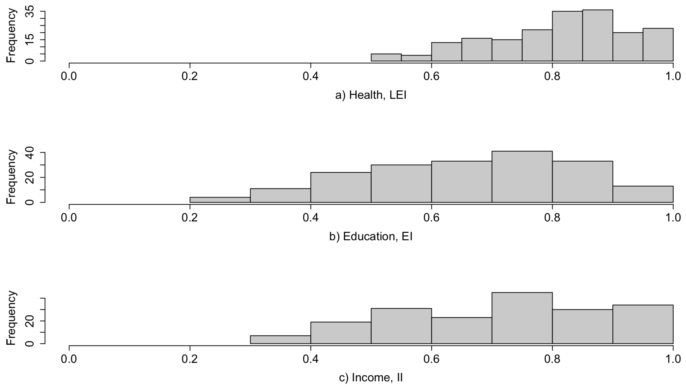
Figure 1 displays the three indicators ($LEI$, $EI$ and $II$) after the normalization process and the aggregation for the education domain. The three normalized indicators exhibit a different distribution. For instance, for the Health dimension ($LEI$), fixing the minimum at 20 years produces a new standardized distribution with $0.51$ as the minimum value, in contrast with the Education dimension ($EI$) that achieves $0.25$.

Table 3. Descriptive statistics for the normalized indicators used to compute the HDI.

Indicator	Mean	St. Dev	Median	Min	Max	Range	Skew	Kurtosis	CV
Health ($LEI$)	$0.81$	$0.11$	$0.83$	$0.51$	$1.00$	$0.49$	$-0.55$	$-0.41$	$13.58\%$
Education ($EI$)	$0.66$	$0.17$	$0.68$	$0.25$	$0.95$	$0.69$	$-0.35$	$-0.77$	$25.76\%$
Economic ($II$)	$0.71$	$0.17$	$0.73$	$0.31$	$1.00$	$0.69$	$-0.24$	$-0.89$	$23.94\%$

reports descriptive statistics for the three normalized indicators.

Although they have different distributions, the three normalized indicators have high levels of correlation: $0.8176$ for the Health and Education indicators, $0.8412$ for the Economic and Health indicators, and $0.8653$ for the Education and Economic indicators.

The HDI for the i-th country is computed as the geometric mean of the three normalized indicators $LEI$, $EI$ and $II$ as follows:

$$\begin{array}{c}\hfill HD{I}_i=\sqrt[3]{{LEI}_i·{EI}_i·{II}_i},i=1,2,\dots ,189.\end{array}$$

(25)

As discussed in the previous sections, the main advantage of the geometric mean is that a poor performance in any dimension is directly reflected in the final value of the indicator. In other words, a low achievement in one dimension is not linearly compensated for by a higher achievement in another dimension. In this way, the level of substitutability between dimensions is reduced and, more importantly, a 1% decline in the indicator of one dimension has the same impact on the HDI as a 1% decline in another one; that is, life expectancy, education and income have the same importance.

5.2. The Computation of the pHDI

Before computing the pHDI through the penalized geometric mean in (17), we check the assumption of Proposition 2. For each country i, we compute its own threshold value, defined as ${\displaystyle z_i^{-}={\mu }_{0,i}exp\left\{\frac{m}{2(m-1)}\right\},}$ $i=1,2,\dots ,189.$ Since here, we have $m=3$ indicators, the threshold value is $z_i^{-}={\mu }_{0,i}{e}^{\frac{3}{4}},$ $i=1,2,\dots ,189.$ The threshold values associated to the countries range in $[0.84,2.03],$ with a mean value of $1.53$ and a standard deviation of $0.32.$

Thus, we look for the countries whose threshold value is lower than 1. Only 11 countries have the threshold value lower than 1; these are: Burkina Faso (27), Burundi (28), Central African Republic (33), Chad (34), Eritrea (55), Mali (107), Mozambique (118), Niger (125), Sierra Leone (153), South Sudan (159), and Yemen (187) (in brackets, the ranking according to the geometric mean). Thus, for those countries, we check if all the values of the indicators constituting the pHDI are less than the threshold value. None of the countries suffers from this limitation.

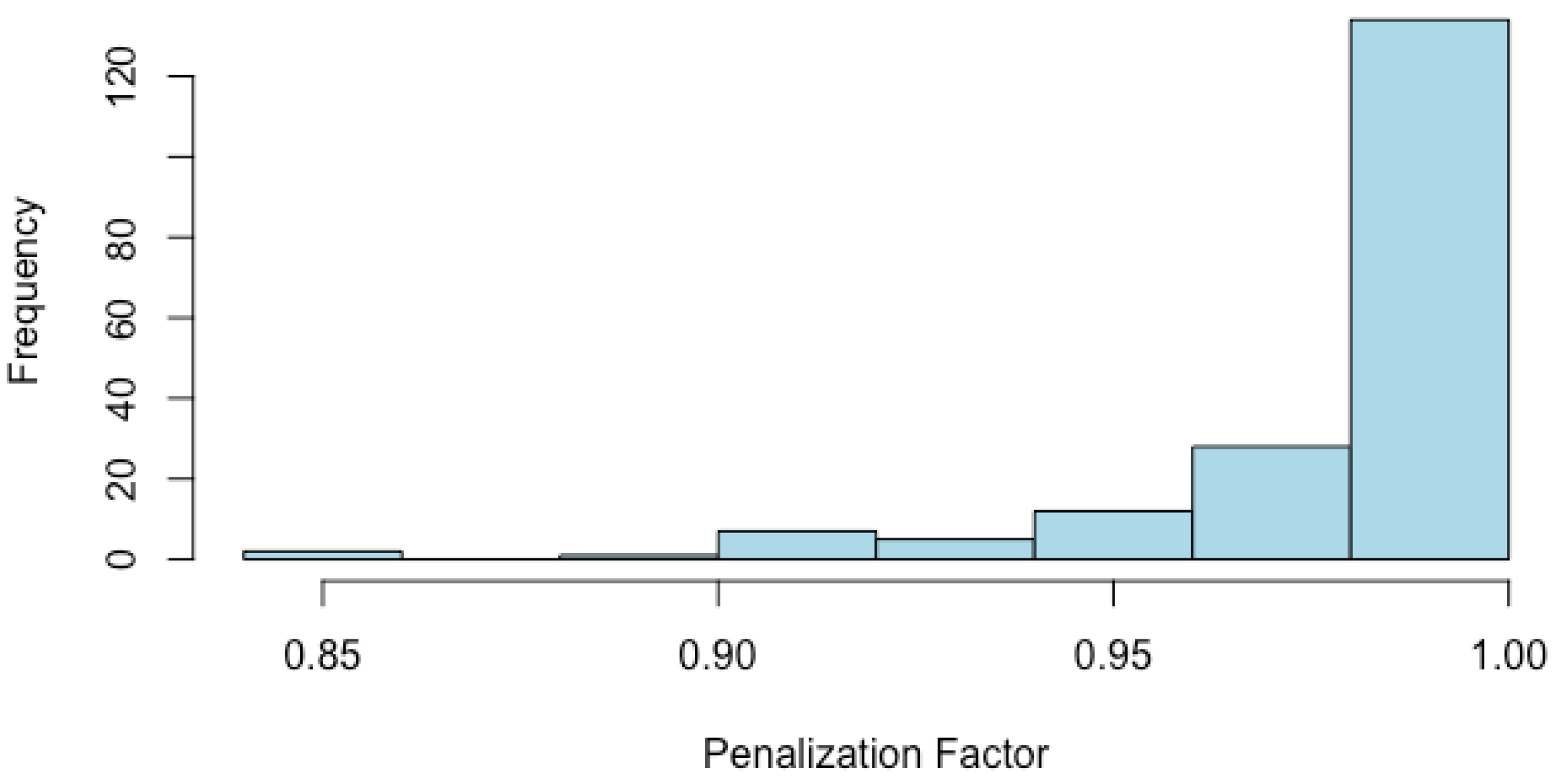
The computation of the pHDI, based on Equation (17), requires the determination, for each country of the penalization factor $exp\{-{\tilde{S}}_{0,i}^2\}$, $i=1,2,\dots ,189$. The penalization factors associated to the countries range from $0.8500307$ (for Eritrea) to $0.9999778$ (for Kazakhstan), with a mean value of $0.9807745.$ As displayed in Figure 2, the distribution of the penalization factor is not symmetric, and $87.83\%$ of its values fall in the range $[0.95,1]$.

5.3. A Comparison between the Two Approaches

Table 4. Descriptive statistics for two methods.

Comp Ind	Mean	St. Dev	Median	Min	Max	Range	Skew	Kurtosis	CV
HDI	$0.72$	$0.15$	$0.74$	$0.39$	$0.96$	$0.56$	$-0.32$	$-0.92$	$20.83\%$
pHDI	$0.71$	$0.16$	$0.74$	$0.34$	$0.96$	$0.62$	$-0.37$	$-0.85$	$22.54\%$

reports descriptive statistics for the geometric mean and the penalized geometric mean approaches. The HDI and the pHDI display similar mean values ($0.72$ and $0.71$, respectively) and the same maximum value ($0.96$) even if the penalized HDI, pHDI, has a wider range than HDI (the minimum value for pHDI is $0.34$ compared with $0.39$ for HDI).

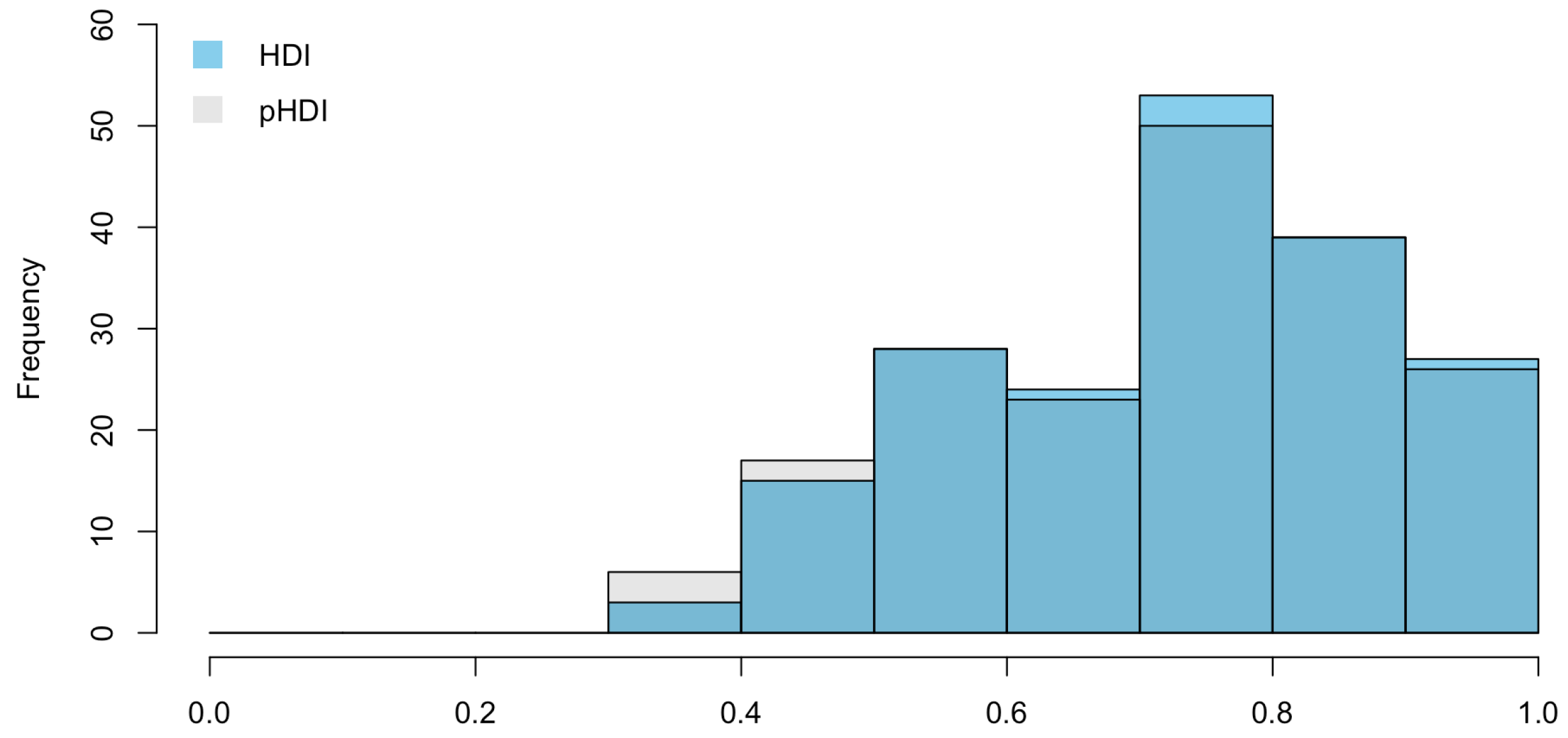
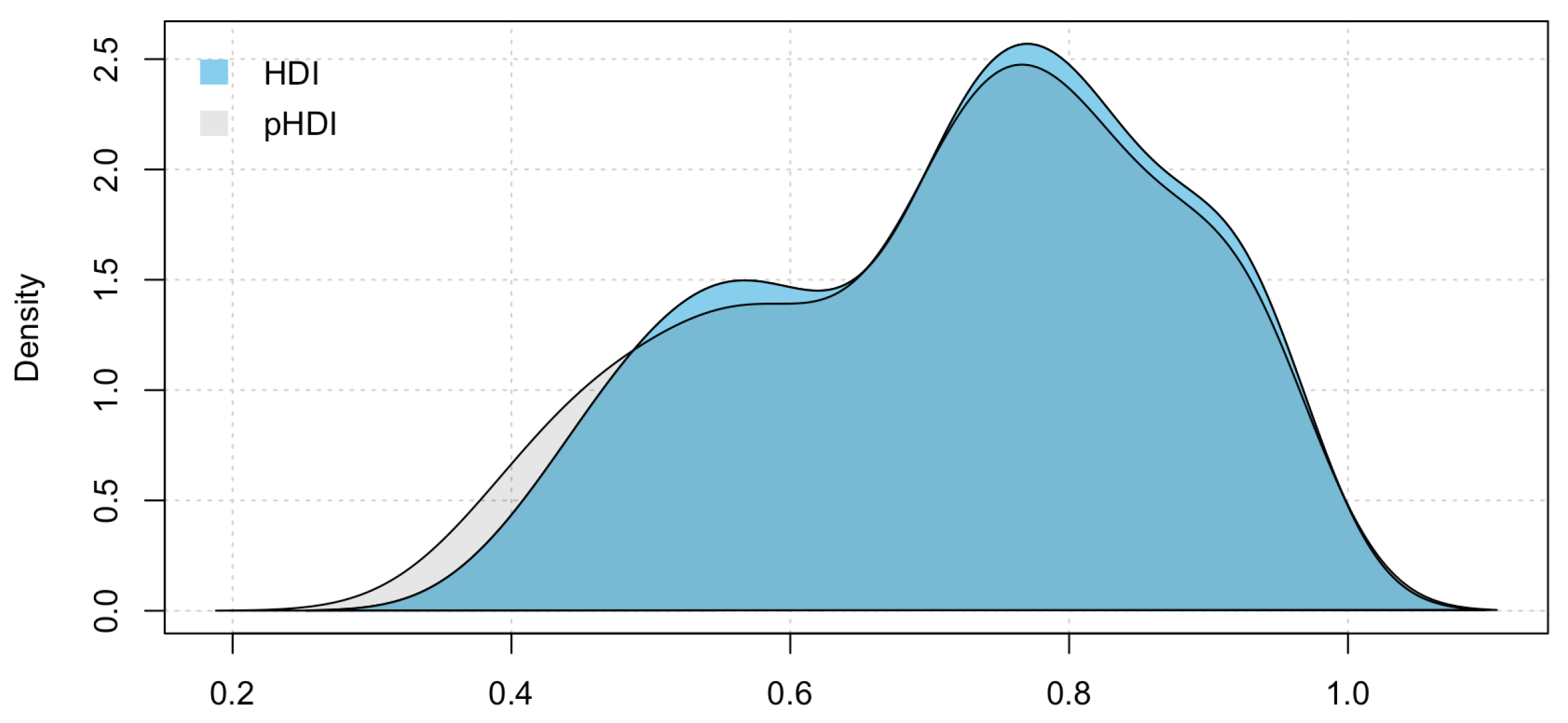
To better compare the values of the two composite indicators, we analyze their distributions (see Figure 3 and Figure 4).

Descriptive statistics, as well as distribution comparison, show a similarity in the distribution of HDI and pHDI, meaning that the addition of the penalization factor in the HDI does not change the distributional feautures. However, since there are (even if small) differences in the range of the two indicators, we compare the corresponding rankings. Firstly, we compute the Spearman’s rank correlation coefficient, which is a simple non-parametric measure of rank correlation, and we test it (Spearman’s rank correlation test). We find a correlation value of $\rho =0.9984554$, and the test suggests that $\rho$ is not equal to 0 with a p-value $<2.2\times {10}^{-16}$.

Then, we compute differences in the ranking position obtained using HDI and pHDI. A positive value of this difference means that country occupies a position according to the HDI better than the position occupied according to pHDI. What emerges is that 42 countries, i.e., $22.22\%$ of the sample, do not change their ranking positions. The percentage of countries that are better ranked by the HDI with respect to its penalized version is $43.39\%$ and, consequently, $34.39\%$ of countries display an opposite behavior. On average, the absolute value of the difference between ranking positions is about $two$ positions.

Table 5. Countries with higher ranking position differences.

Country	HDI	pHDI	Difference
Maldives	95	110	−15
Syrian Arab Republic	151	161	−10
Qatar	45	53	−8
Lebanon	92	100	−8
Cuba	70	77	−7
Armenia	81	75	6
Mongolia	99	93	6
Lesotho	165	159	6
Guinea-Bissau	177	170	7
Nigeria	161	153	8

reports the ranking positions of the countries with higher (positive and negative) differences between the two methods.

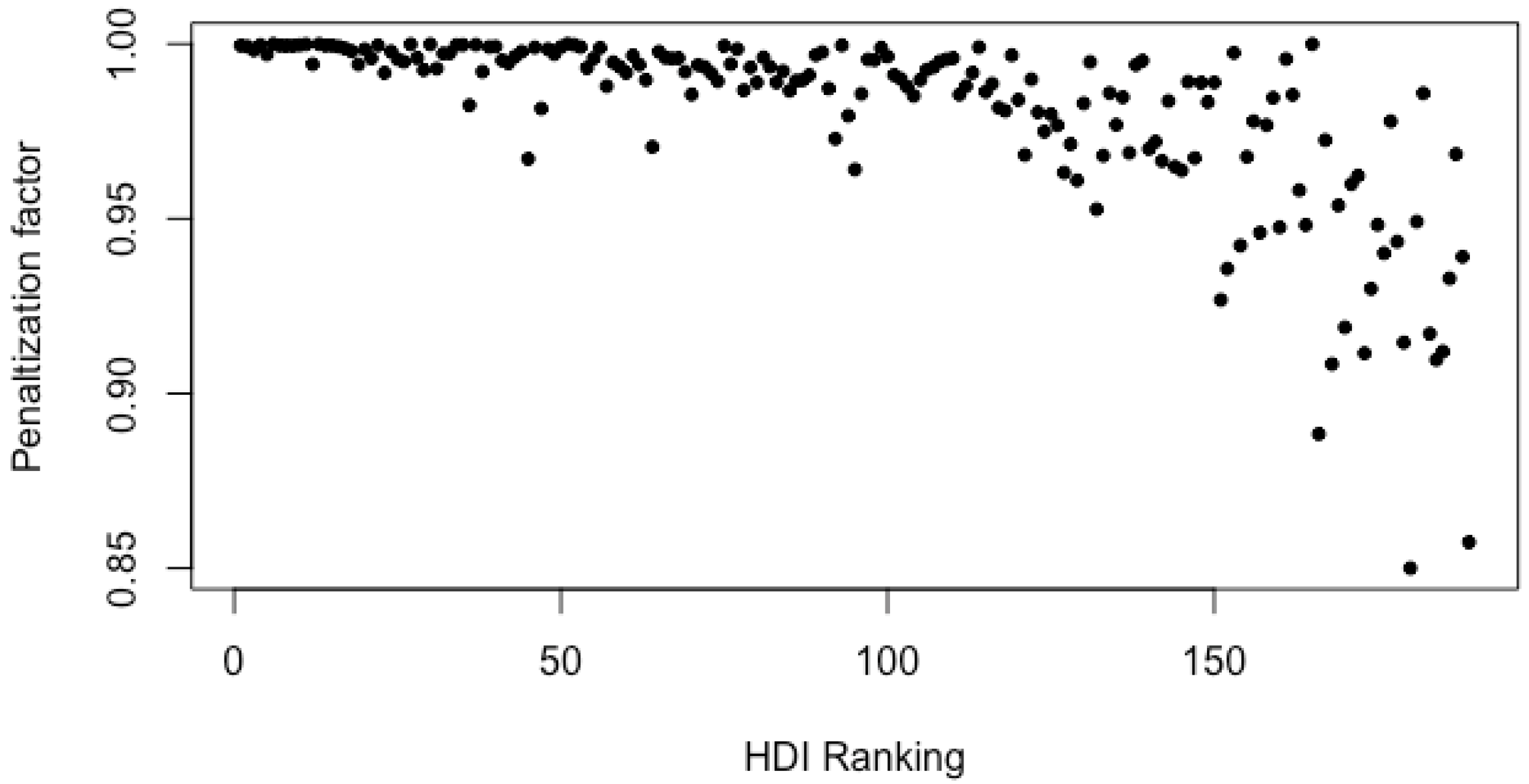
To investigate in depth the size of the penalization factor, we plot its values as a function of the HDI ranking position (see Figure 5). The plot reveals that the size of the penalization is higher for high ranked countries; this means that the greater the HDI ranking position of the country, the greater the penalization suffered using pHDI instead of HDI.

The greater impact, which corresponds to the smaller values for penalization factor, is attributed to Eritrea, that in the original ranking of HDI occupies the position 180, whereas the smaller impact is achieved by Kazakhstan with a penalization factor of $0.999977836$ (ranked 51 in the HDI ranking) followed by Germany with a penalization factor of $0.999975672$ (ranked 6 in the HDI ranking).

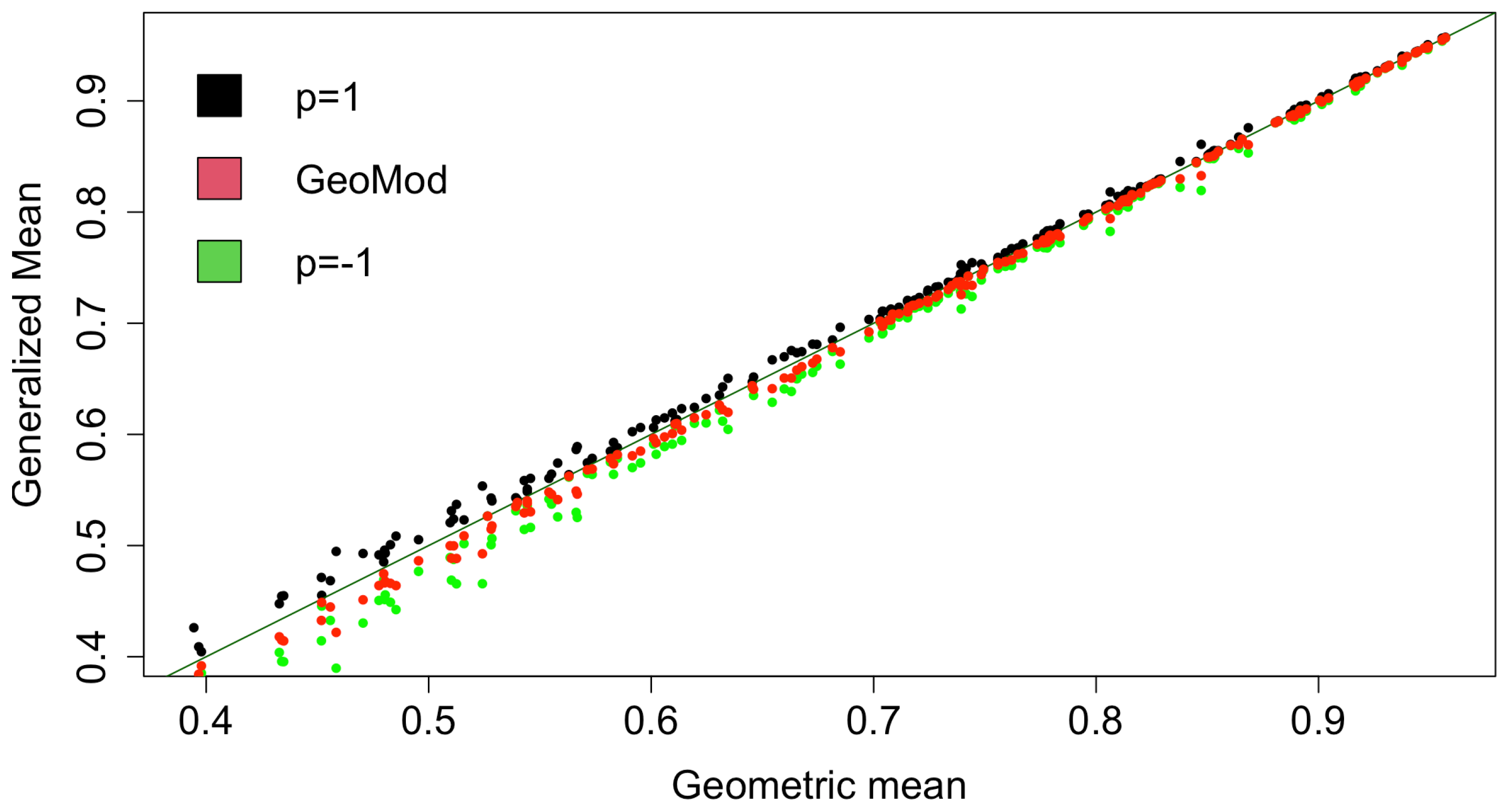
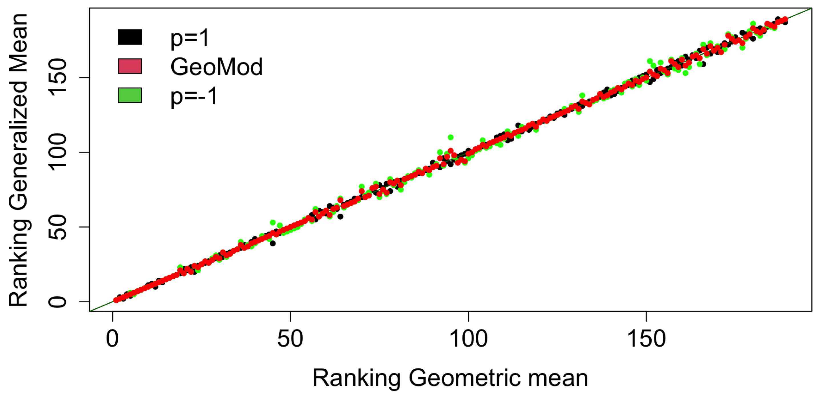
Finally, in order to investigate the role of the aggregation method used, we study the relationship between HDI and pHDI using as benchmarks two other versions of the HDI obtained aggregating the Health, Education, and the Income indicators with the generalized mean of order $p=-1$ (the harmonic mean) and $p=1$ (the arithmetic mean). We have chosen the harmonic mean because this approach, as with the pHDI, introduces a downward penalization for unbalanced indicator values. Specifically, in Figure 6, we plot the values of three versions of the HDI obtained with the harmonic mean ($p=-1,$ in green), the arithmetic mean ($p=1,$ in black) and the penalized geometric mean (in red) versus the values of the HDI obtained with the geometric mean. In Figure 7, we plot the ranking positions obtained with the harmonic mean version of the HDI ($p=-1,$ in green), with the arithmetic mean version of the HDI ($p=1,$ in black) and with the pHDI (in red). In both the figures, to highlight the difference of the three HDI versions with respect to the geometric mean version, we plot the strength line of equality.

Figure 6 shows that the penalization introduced in the pHDI gives values of the composite indicator that are less than those produced by the harmonic mean approach, especially for the countries with lower values of HDI. Contrarily, the countries with larger values of HDI have similar values for the other versions of the HDI. This behavior is confirmed by Figure 7, where we can see that the HDI top-ranked countries are closer to the line of equality, meaning that the top ranked countries are less influenced by the choice of the aggregation method. All these findings reveal that, differently from those at the bottom and in the middle, the countries on the top of the HDI ranking have highly balanced values of the indicators constituting the HDI; moreover, the pHDI penalizes more than the harmonic mean approach.

6. Conclusions

A composite indicator is a mathematical combination of a set of indicators. The crucial aspect is the choice of the aggregation function to use. There is not universal agreement on the aggregation method to use even if the criterion that must guide the choice is the ease of computation.

The simplest aggregation function is the arithmetic mean. Despite its ease of computation, it has the major drawback due to substitutability between indicators. A possible way to overcome this limitation consists of introducing, for each unit, a penalization factor that accounts for the horizontal variability among indicators. This is the idea behind the Mazziotta and Pareto aggregation method. Keeping this idea in mind, in this paper, we propose a theoretical method for penalizing the geometric mean, by means of a penalization term that measures the horizontal variability among the normalized indicators opportunely transformed applying the Box–Cox function of order zero. The introduction of a penalization allows capturing the unequal distribution of achievements within the country and, consequently, gives a more accurate picture of the differences among countries.

The empirical part highlights our proposal by comparing the classical HDI with its penalized version, namely the pHDI, for 189 countries in 2019. The comparison between the two methods reveals that the new method does not upset the ranking provided by the geometric mean and impacts more for countries with poor performances. The method proposed here to penalize the geometric mean could be generalized for any member of the family of generalized means. This awaits further research.

References

- OECD/European Union/EC-JRC. Handbook on Constructing Composite Indicators: Methodology and User Guide; OECD Publishing: Paris, France, 2008; Available online: https://0-www-oecd--ilibrary-org.brum.beds.ac.uk/economics/handbook-on-constructing-composite-indicators-methodology-and-user-guide_9789264043466-en (accessed on 28 February 2022).
- Berger, R.L.; Casella, G. Deriving Generalized Means as Least Squares and Maximum Likelihood Estimates. Am. Stat. 1992, 46, 279–282. [Google Scholar]
- Mazziotta, M.; Pareto, A. A non-compensatory approach for the measurement of the quality of life. In Quality of Life in Italy; Springer: Dordrecht, The Netherlands, 2012; pp. 27–40. [Google Scholar]
- Ijiri, Y. Fundamental Queries in Aggregation Theory. J. Am. Stat. Assoc. 1971, 66, 766–782. [Google Scholar] [CrossRef]
- UNDP. Human Development Report 2010: The Real Wealth of Nations—Pathways to Human Development; UNDP: New York, NY, USA, 2010; Available online: http://hdr.undp.org/en/content/human-development-report-2010 (accessed on 28 February 2022).
- UNDP. Human Development Report 2007/2008-Fighting Climate Change: Human Solidarity in a Divided World; UNDP: New York, NY, USA, 2007; Available online: https://hdr.undp.org/sites/default/files/reports/268/hdr_20072008_en_complete.pdf (accessed on 28 February 2022).
- Box, G.E.P.; Cox, D.R. An analysis of transformations. J. R. Stat. Soc. Ser. B 1964, 26, 211–252. [Google Scholar] [CrossRef]
- Casadio Tarabusi, E.; Palazzi, P. An index for sustainable development. BNL Q. Rev. 2004, 229, 185–206. [Google Scholar]
- Casadio Tarabusi, E.; Guarini, G. An unbalance adjustment method for development. Soc. Indic. Res. 2013, 112, 19–45. [Google Scholar] [CrossRef]
- El Gibari, S.; Gomez, T.; Ruiz, F. Building composite indicators using multicriteria methods: A review. J. Bus. Econ. 2019, 89, 1–24. [Google Scholar] [CrossRef]
- Lai, E.; Lundie, S.; Ashbolt, N.J. Review of multi-criteria decision aid for integrated sustainability assessment of urban water systems. Urban Water J. 2008, 5, 315–327. [Google Scholar] [CrossRef]
- Azapagic, A.; Perdan, S. An integrated sustainability decision-support framework Part II: Problem analysis. Int. J. Sustain. Dev. World Ecol. 2005, 12, 112–131. [Google Scholar] [CrossRef]
- Charnes, A.; Cooper, W.W.; Rhodes, E.L. Measuring the efficiency of decision making units. Eur. J. Oper. Res. 1978, 2, 429–444. [Google Scholar] [CrossRef]
- Diaz-Balteiro, L.; Gonzalez-Pachon, J.; Romero, C. Measuring systems sustainability with multicriteria methods: A critical review. Eur. J. Oper. Res. 2017, 258, 607–616. [Google Scholar] [CrossRef]
- Roy, B. The outranking approach and the foundations of ELECTRE methods. Theory Decis. 1991, 31, 49–73. [Google Scholar] [CrossRef]
- Brans, J.P.; Vincke, P.; Mareschal, B. How to select and how to rank projects: The PROMETHEE methods. Eur. J. Oper. Res. 1986, 24, 228–238. [Google Scholar] [CrossRef]
- Greco, S.; Ishizaka, A.; Tasiou, M.; Torrisi, G. On the methodological framework of composite indices: A review of the issues of weighting, aggregation, and robustness. Soc. Indic. Res. 2019, 141, 61–94. [Google Scholar] [CrossRef] [Green Version]
- Mazziotta, M.; Pareto, A. Un indicatore sintetico di dotazione infrastrutturale: Il metodo delle penalità per coefficiente di variazione. In Proceedings of the Lo Sviluppo Regionale nell’Unione Europea-Obiettivi, Strategie, Politiche, Atti della XXVIII Conferenza Italiana di Scienze Regionali, Bolzano, Italy, 28–28 September 2007; Available online: https://aisre.it/images/old_papers/Mazziotta-Pareto.pdf (accessed on 28 February 2022).
- Mazziotta, M.; Pareto, A. On a generalized non-compensatory composite index for measuring socioeconomic phenomena. Soc. Indic. Res. 2016, 127, 983–1003. [Google Scholar] [CrossRef]
- Noorbakhsh, F.A. modified human development index. World Dev. 1998, 26, 517–528. [Google Scholar] [CrossRef]
- Paul, S. A modified human development index and international comparison. Appl. Econ. Lett. 1996, 3, 677–682. [Google Scholar] [CrossRef]
- Jha, R.P.; Bhattacharyya, K.; Mishra, D.; Pedgaonkar, S.P. Health Adjusted Human Development Index: A Modified Measure of Human Development. Int. J. Health Sci. Res. 2017, 7, 207–220. [Google Scholar]
- Prados de la Escosura, L. Improving human development: A long-run view. J. Econ. Surv. 2010, 24, 841–894. [Google Scholar] [CrossRef] [Green Version]
- Chakravarty, S.R. A generalized human development index. Rev. Dev. Econ. 2003, 7, 99–114. [Google Scholar] [CrossRef]
- Alkire, S.; Foster, J.E. Designing the Inequality-Adjusted Human Development Index; OPHI Working Paper Series; 2010; Volume WP37, Available online: https://www.ophi.org.uk/wp-content/uploads/ophi-wp37.pdf (accessed on 28 February 2022).
- Mazziotta, C.; Mazziotta, M.; Pareto, A.; Vidoli, F. La sintesi di indicatori territoriali di dotazione infrastrutturale: Metodi di costruzione e procedure di ponderazione a confronto. Riv. Econ. Stat. Territ. 2010, 1, 7–33. [Google Scholar] [CrossRef]
Figure 1.
(a) Distribution of the Health indicator (). (b) Distribution of the Education indicator (). (c) Distribution of the Economic indicator ().
Figure 2.
Distribution of the penalization factor.
Figure 3.
Frequency histogram of HDI and pHDI.
Figure 4.
Density distribution of HDI and pHDI.
Figure 5.
Penalization factor vs. HDI ranking.
Figure 6.
Scatter plot of the harmonic mean version (in green), the arithmetic mean version (in black) of the HDI and the pHDI values (in red) vs. the HDI values.
Figure 7.
Scatter plot of the ranking obtained with the harmonic mean version of HDI (in green), with the arithmetic mean version of HDI (in black) and with the pHDI (in red) vs. the ranking obtained with HDI ranking.