1. Introduction
Many processes lead to gene trees that differ from species trees. These processes include gene duplication and loss, lateral gene transfer and incomplete lineage sorting, in addition to phylogenetic errors in gene tree reconstruction [
1,
2]. Interest in identifying and understanding these processes by comparing gene trees with species trees is growing. Gene duplication and retention/loss after duplication is one area that has received particular attention in model development, both mechanistic and phenomenological. A general discussion of the use of mechanistic
vs. phenomenological models for problems in genomics has recently been published [
3], and this paper follows up with a more technical discussion on the development and interpretation of models for duplicate gene retention/loss.
Dating back to Ohno [
4], it was realized that gene evolution in the absence of gene duplication was conservative, with any functional shifts concurrent with negative (stabilizing) selection to retain existing gene functions. Gene duplication itself was thought to be important as a process that enabled amino acid substitution to explore protein function space under relaxed constraints with redundant copies in a genome to perform key functions. In bioinformatics analysis, this hypothesis led to the development of an entire field of orthology prediction, with the view that orthologs were more likely to have retained function, whereas paralogs (products of duplication) were more likely to have diverged in function. The process of gene tree/species tree reconciliation emerged as one of the leading methods for differentiating between orthology and paralogy, with explicit consideration of phylogenetic structure. With the acknowledgment of the possibility of functional shifts in orthologs, various types of rate shift analysis became common in evaluating lineage-specific functional change/conservation. Similarly, in the emerging gene duplication field, the relationship between duplication and function was analyzed in more detail. A more mechanistic trajectory for studying gene duplicates emerged with the seminal papers of Lynch and Force (for example, [
5]). The development of tractable models that enable the probabilistic testing of mechanistic hypotheses emerged as a research trajectory.
Several processes lead to the retention of genes with a decreased probability of loss. All of these retention processes play out against a neutral backdrop, leading to nonfunctionalization (the generation of nonfunctional gene copies from the process of amino acid substitution). In the substitution-based processes that are being modeled, there is a constant rate of accumulation of deleterious substitutions that lead to duplicate gene loss of functionally-redundant copies. This process occurs simultaneously with processes that lead to loss of redundancy and a higher rate of gene retention. The nonfunctionalization rate itself depends on the degree of redundancy and other selective forces. Neofunctionalization is one alternative process for retention that involves a new function emerging in one gene copy, while the other copy retains the ancestral function [
4]. Subfunctionalization is another process that involves the neutral division of functions from a multifunctional ancestral state through substitutions that cause partial functional loss, but are neutral in the context of redundancy [
5]. Dosage balance is a third process that leads to modified loss dynamics and involves the co-retention of duplicate genes that interact as proteins and are in stoichiometric balance, but become deleterious when out of stoichiometric balance [
6]. There are other processes and many variations on these themes (see [
7]).
This manuscript presents three distinct modeling frameworks. The first framework models average retention properties as survival functions. The second framework extends this analysis, while treating retention processes as distinct from the ongoing loss processes that occur simultaneously (whereas these are averaged together in the first modeling framework). A third framework also builds upon the first framework, towards a phylogenetic birth-death model. The first framework (in
Section 2,
Section 3,
Section 4,
Section 5,
Section 6,
Section 7,
Section 8 and
Section 9) represents a clarification of published work, while the second (
Section 10) and third (
Section 11) frameworks are presented conceptually and mathematically, with an implementation in the process of being published elsewhere.
2. Mechanistic Models for Describing Retention Probabilities as Average Survival Functions
Initial and non-mechanistic or approximate characterizations of gene loss relied upon an exponential distribution of retention (where the retention probability is a one-loss probability), implying a constant rate of loss until all duplicates are lost [
8,
9]. This model is unintentionally consistent with the nonfunctionalization process. In Equation (1), the probability of survival of a gene to at least time
t (denoted
S(
t)) depends upon the hazard rate d, which describes the constant instantaneous rate of loss.
A first step towards mechanistic justification of a model was to enable loss rate decay with a Weibull distribution [
10]. In this context, the Weibull distribution is mechanistically inspired by the need for a decaying loss rate associated with the neofunctionalization process occurring simultaneously with the nonfunctionalization process. A Weibull function does not present a generative model for the retention of genes that are neofunctionalizing, in the sense that it is a true biological description of the survival probability given the simultaneous action of nonfunctionalization and neofunctionalization. The relationship between the underlying biology and the waiting time for a single event is reflected in the dynamics of the waiting time for an adaptive substitution that drives retention through neofunctionalization. Averaging over such waiting times, while loss is occurring, due to the accumulation of nonfunctionalizing changes, leads to the Weibull function, as described in [
10]. In Equation (2),
S(
t) depends upon parameters
d1 and
d2, where
d2 modulates the time-dependence of the loss process and values between zero and one are consistent with averaging across waiting times for a single event, such as a neofunctionalizing substitution.
The hazard function of Equation (2) when
d2 has a parameterization between zero and one shows concave decay. Another type of decay of the loss rate involves a convexly decaying hazard rate that is not parameterizable with a Weibull distribution, and that would be consistent with a waiting time for multiple deleterious, but non-lethal events, such as subfunctionalizing events, while nonfunctionalizing substitutions also occur as a background process. As shown in Figure 7 of [
10], the convex decay originates from the waiting time for multiple events, as opposed to a single beneficial change in the neofunctionalization model, where the exact curve shape depends upon the number and type of elements to be subfunctionalized. The dosage balance mechanism was proposed to be consistent with a concavely increasing loss rate based upon the expectation of the stochastic deleterious loss of one partner, leading to the cooperative loss of the remaining duplicates [
11]. Konrad
et al. [
12] then derived a more complex distribution that could accommodate curve shapes consistent with all of the four mechanisms described above (nonfunctionalization (constant loss rate), neofunctionalization, dosage balance and subfunctionalization) and their proposed mathematical correlates.
3. The Konrad Model and Its Implementation
The hazard function for the Konrad
et al. [
12] model is described below together with its accompanying survival function. In the hazard function (and corresponding survival function), the
b and
c parameters describe the rate of change of the hazard rate, as well as its convexity/concavity,
f +
d describes the instantaneous hazard rate and d describes the asymptotic hazard rate. An exponential function will just require a
d parameter, obtained when
f = 0. The survival function is derived from the hazard function in relating the accumulation of instantaneous rates of loss until time
t to the probability of surviving to at least time
t.
Building upon the Hughes and Liberles [
10] study, in addition to the Konrad
et al. [
12] model, Denoeud
et al. [
13] described another modeling approach that was validated through goodness-of-fit tests. The approach in Denoeud et
al. [
13] generated a mixture of two Weibull distributions and a single discrete distribution to fit the data. These two modeling strategies will be discussed in consideration of the data and the inference of biological processes that are made.
It should be noted that in these studies, bioinformatics pipelines were generated that fit dS (the rate of synonymous change that, if neutral, reflects mutational opportunity accumulating in a clocklike manner) histograms generated from intra-genomic analysis involving BLAST hits. This built upon an analysis framework that was designed by Lynch and Conery [
8] and represented a logical step in model validation before extending models to a phylogenetic context. From the BLAST hits, a pipeline was introduced that collects genes present in an extant genome and results in pairwise dS values reflecting the time that the genes have survived since duplication. In the histogram plots, the genes are binned into collections of genes of similar age (dS value). While there has been some discussion of methodological choices in this framework, this will be briefly entertained without becoming the focus of the presentation.
4. A Brief Technical Discussion of Data Fitting and Truncation
In the Konrad
et al. [
12] analysis, survival functions were fit to the observed time-dependent survival of duplicates, either from comparative genomics or from simulations, with the assumption that counts of duplicates observed at each time point were independent of counts observed at each other time point. This assumption was met for the comparative genomic data, where the genes are samples (cohorts) of duplicates of different ages in present day genomes, but not the simulated data used in Konrad
et al. [
12], where this was an approximation. The fit to the data was based upon the least squares fit of the survival data (for each cohort) as the probability of being alive at time
t (the median age of the cohort), given birth at
t = 0. With an assumption of constant duplication rates, as described below, each cohort is expected to be of equal size. Correspondingly,
S(0) = 1. If no loss occurs, the size of each bin is expected to be the same, one (or scaled to
N0, the parameterized estimate of the initial number of duplicate genes at
t = 0). The various generations of
S(
t), including their use and equivalence, are shown in
Figure 1. Extension of this model to a phylogenetic framework can be made in terms of likelihood statements of observations of retention and loss over species tree branch lengths or as a full phylogenetic birth-death model.
Figure 1.
(A) The probability density function (PDF) for a Weibull distribution is shown; (B) the PDF of the right truncated Weibull with the same parameters is shown, where data beyond dS = 0.3 is not collected; (C) The cumulative density function (CDF) for the PDF in (A) is shown, indicating the assumed loss associated with gene duplicates not observed at various ages; (D) Identical to the cdf in the lower left quadrant of (C) is the right truncated CDF derived from the PDF in (B), (E); The survival function associated with (A) and (C) is shown. The value at dS = 0 is defined and equal to one, indicating that at the point of birth, all duplicates still survive; (F) The survival function associated with the right truncated distributions in (B) and (D) is shown. This plot is identical to the upper left quadrant of (E).
In fitting the model, sub-model fit was performed independently across model parameterization ranges consistent with each biological mechanism, with likelihood scores compared using AIC to give a maximum likelihood identification of the parameter range (biological model). AIC was not corrected for differences in the effective number of parameters from the true number of parameters from restricting the allowable range of all parameters to values that had a biological interpretation.
In statistics, models for the error between the expected number of counts and the observed number of counts can be important to proper inference and need attention together with the mechanistic model itself, both for
dS data and ultimately in a phylogenetic context. The observed count
xi of gene copies within time interval for genes with age
i can be treated as a Poisson distribution with mean
θi =
N0S(
ti) (Equation (5)). The Poisson error function is not right truncated and examines error in the
y-axis between the predicted value of the model with parameterization and the observed data when fit with
S(
t), formulated as a likelihood. In the Equation (6) below, the chi-square statistic is the sum of squared errors between the observed number
xi of gene duplicate counts at time
ti and the expectation for that number of counts from the survival function as the parameter estimate of the starting number of genes at
t = 0 (
N0) and the probability of that number of genes surviving to at least
ti, S(
ti). Model parameterization can be generated with different error models using a differential evolution approach [
14]. Genetic algorithms were found, as expected, to outperform hill climbing strategies in avoiding local optima on complex surfaces, like those associated with the General Death Model (GDM) model on survival data.
While the data are right truncated, given that S(t) was not a probability density function and integrated over the hazard of being lost between t = 0 and t, the expectation at t is independent of the measurement of time points beyond t, and no correction for right truncation is needed. With an assumption of a constant birth rate, the genes in Bin 1 reflect the equally-sized cohort of genes observed at Age 1 that were duplicated in a given constant time window in the past. The genes in Bin 2 reflect the equally-sized cohort of genes observed at Age 2 today that were duplicated in that given constant window in the past. Truncation at bin x results in the absence of bins t > x, but does not affect the number of genes in any bin t < x for genes that are duplicated at time t and survived to at least the present.
The mathematical relationship between the approaches is shown in
Figure 1. Studies by Lynch and Conery [
8], Lynch and Conery [
15], Hughes and Liberles [
10] and Konrad
et al. [
12], as suggested above, fit the survival function shown in
Figure 1E, with the assumption of a constant birth rate, generating an equivalent number of duplicates, where loss over the period accounts for the declining numbers of genes. An alternative mechanism to fit the data is to use the right truncated probability density function shown in
Figure 1B derived with the associated cumulative loss function in
Figure 1D. The probability density function in
Figure 1B, which was not used to fit data, does not account for right truncation at
t = 0.3 and assumes that no duplicates survive beyond
t = 0.3.
Figure 1C,E show the survival of duplicates beyond
t = 0.3, associated with the different approaches, generating the equivalence of
Figure 1E,F. The assumptions involved in extending this analysis to a phylogenetic context depend upon how the phylogenetic model is constructed, but in the simplest case, it can be directly applicable, where a gene that appears in the leaf set has survived for at least the time since the duplication event time. A fuller phylogenetic birth-death model is described later in this manuscript.
6. Model Selection and Model Expansion
The Konrad
et al. [
12] model was originally fit with four distinct parameter ranges. Datasets involving two hybrid processes, dosage balance plus neofunctionalization and dosage balance plus subfunctionalization, were forced to fit one of the processes independently. These processes reflect
a priori hypotheses about mechanism, and model selection is only among these
a priori hypotheses. This should be reflected in the fit of the best model to the data. Testing
a priori interpretable hypotheses through model selection is a valid scientific approach. Of course, there is always the caveat that none of the models being specified
a priori reflects the true biological mechanism at the desired level of inference.
In Konrad
et al. [
12], all of the datasets were fit to one of the processes that were consistent with the underlying simulation mechanism, and no problem was foreseen. Subsequently, it was realized that the prolonged retention through the dosage balance mechanism could cause dosage balance plus either subfunctionalization or neofunctionalization to be misparameterized. The model needs expansion to incorporate those two processes (dosage plus subfunctionalization and dosage plus neofunctionalization) independently and to generate six total processes, the next step in the progression of models. These models are currently under development and will be described elsewhere. Additional testing of the identifiability of the model or a derivative model is necessary to ensure both statistical and biological identifiability (see [
3]). The concept of biological identifiability is introduced in the use of biologically realistic simulation under unrelated models to validate the mechanistic predictions (for example, using an ROC curve) as a complement to goodness-of-fit tests.
Ultimately, the modeling approach made a number of assumptions about the underlying biology that need to be evaluated. Effective population sizes (and fluctuating versions of them) were not incorporated into the model. One mechanism that can give a population size-dependent effect is failed fixation (loss due to population dynamics). In general, inter-specific modeling has treated substitution processes as a Markov process in sampling a single individual from multiple species. It has been noted that this experimental design includes a mix of segregating variation and fixed change, where the ratio between the two is dependent upon the branch length. Not accounting for segregating variation in Markov processes may be a problem in general in phylogenetics, including the modeling of gene duplication and loss.
Similarly, the processes were simulated as initially fixed in a haploid organism rather than introduced to a single chromosome of a diploid organism, which might be more relevant to metazoan or embryophyte species, where duplication is commonly studied (see [
16]). In fitting genomic data, birth rates were assumed constant, but this assumption is almost certainly violated [
17]. Additionally, co-evolution of processes and levels of biological organization (concentration through gene expression and dosage, for example) were not considered as a possibility. Partial birth events that give rise to genes that are born neo- or sub-functionalized were not considered [
18]. Lastly, how gene conversion events [
19] are viewed in the context of this modeling framework as a process that might lead to simultaneous birth and loss, including hybrids of duplicates with newer and older pieces, should be considered. The effects of all of this biological realism are ultimately important to evaluate. Some of the biological realism was described in the early work of Lynch
et al. [
5]. However, the models described in that paper are even more complex than those used by Konrad
et al. [
12] without accounting for all of the processes.
8. Inference of Instantaneous Duplication and Loss
One assumption of the approach is that loss is described by the accumulation of non-synonymous substitutions that occur together with the faster accumulation of synonymous substitutions. This assumption would lead to negligible instantaneous loss at dS = 0 and suggests that dS as a measure of mutational opportunity is the appropriate clock in which to tick for the loss processes. Besides the genome annotation artifact [
20], one distinct process that would lead to a distinct rapid loss process is failed fixation or fixed deletion events. This process was discussed by Konrad
et al. [
12] and evaluated with the assumption of an initially fixed duplication event. The process of fixation of a duplication event occurring in a single individual was not evaluated and is discussed below. However, inference of loss according to this process and data-fitting using a discrete process at dS = 0 and a mixture of Weibulls at dS > 0 that account for this process plus nonfunctionalization rather than a coalescent process that models population dynamics has not fully been evaluated for biological accuracy (would a discrete point process rather than a loss process based upon theoretical expectations of failed fixation and fixed loss events properly count the number and rate of such events?). Loss events at dS = 0 are not directly observed, and the evidence for them comes from model fit. It is unclear if the inference would change by applying a third Weibull component to fit rapid loss or another combination of phenomenological distributions, rather than a discrete distribution at
t = 0 in combination with two Weibull distributions. The application of the mixture implies a distinct or discontinuous process if the model is to be interpreted as a loss hazard that is not fit by a Weibull. Understanding this process and what is being fit is important to progress in the field. It is likely that much of the difference in parameterization of the Denoeud
et al. [
13] decay and the Konrad
et al. [
12] decay relates to the introduction of the discrete distribution at discontinuously fit loss at
t = 0, and understanding what this is fitting will be critical to biological interpretation of the hazard function parameterization.
In interpreting a mixture of Weibull distributions, one that decays and one that does not, it is not necessarily the case that one is fitting purely a loss process and the other the duplication rate (or loss rate) heterogeneity, although that is likely to be part of the fit. What is more controversial is the comparison of the product of the mixture modeling to describe the hazard function and comparing with a hazard that is constrained to fit loss. It is unclear what the hazard from the Weibull mixture model is fitting and, therefore, how to interpret it. The Weibull component that exhibits decay may be describing a loss process in the data, but it is also unclear what this means in combination with the second Weibull component.
In Liberles
et al. [
3], a model is described where a non-constant birth process and a single Weibull are simulated. The generative parameterization of the Weibull loss function is not recovered through fitting with a mixture of Weibull components, not in the composite distribution or in any of the individual distributions. This has broad implications for data interpretation using mixtures of processes where the goal is the use of mechanistic parameter values to make inference, both because of the potential interplay of phenomenological and mechanistic parameters and because of problems in inference with misspecified models (for example, assuming a constant birth rate when there is none). It is likely the case that such models may still be biologically identifiable (recovering the correct biological mechanism) even when not fully statistically identifiable, but this statement will require more careful examination to support.
9. The Future of Duplication and Loss Modeling
Ultimately, duplicate gene retention or loss is complex and is only one part of the puzzle. The analysis introduced by Lynch and Conery [
8] and extended by Hughes and Liberles [
10] is approximate in several ways. Basing the analysis on pairwise dS values for duplicates rather than from phylogeny has the potential to miscount duplicate numbers with a bias that increases with the age of the pair and relates to the symmetry of the underlying tree. This is shown in
Figure 3. Secondly, dS is used as a proxy for time or, more directly, mutational opportunity, with an assumption of dS neutrality. Recent work has suggested that dS is not neutral, but under selection for several mechanistic reasons [
21]. While a neutral mutational clock would be appropriate, it is unclear that external sources of geological time would be appropriate clocks in which to tick for the loss rate. On the other hand, population genetic processes related to (for example) failed fixation should probably click in generation time as a scalar of geological time.
Figure 3.
(
A) A phylogenetic tree showing the relationship of and distances between duplicated genes in a gene family; (
B) the corresponding histogram based upon the best BLAST hits for a duplicate is shown. The duplication event at dS = 0.5 would be missing from the data. The frequency of such missing data increases dependent on tree symmetry with increasing time, leading to the justification of right truncation at dS = 0.3 as a reasonably powerful, fast approximate analysis (Lynch and Conery [
8]; Hughes and Liberles [
10]). Branch lengths are drawn to scale, with branch lengths labeled in dS units (substitutions per site).
This does not mean that the types of models being developed are useless. Phylogenies can be evaluated to provide duplicate gene survival and loss times and the probabilities for such events associated with alternative parameterizations of the model. Alternatively, full phylogenetic birth-death models with gene family sizes can be calculated with an appropriate distribution. This necessitates the development of gene tree-species tree reconciliation frameworks with biologically-realistic models, where the reconciliation and species tree branch lengths (or even topology) are also evaluated. More complexity in the duplication process, including rate variation, and the necessity of whole genome duplication events for the validity of the dosage balance model will be important developments. It also remains to be explored when complexity in both the duplication and loss scenarios will result in models that are not identifiable. The next part of the manuscript will extend current models, ultimately as birth-death models with time heterogeneous loss functions, as the next step in moving forward.
10. Towards a New Time Heterogeneous Markov Model for Gene Duplication
The current modeling framework has resulted in a time-heterogeneous process that combines nonfunctionalization with retention processes. One strategy might be to generate a new Markov model that is a mix of time homogeneous and time heterogeneous processes. A scheme for doing this is presented in
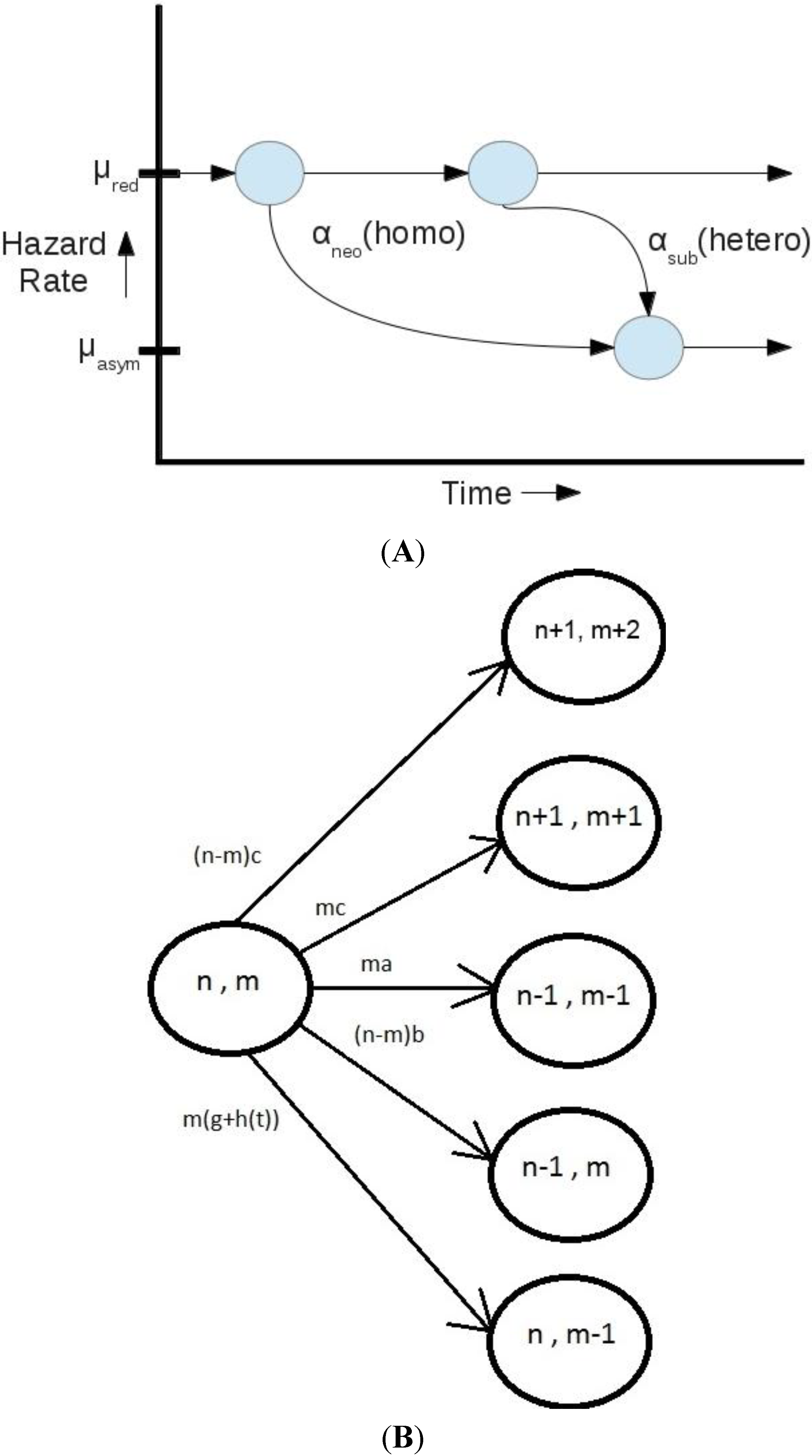
Figure 4A,B, focused on the loss and retention processes, where duplication can easily be added as a birth-death model. The model in Equations (3) and (4) is designed to treat an average of multiple genes based upon an expectation of nonfunctionalization as a constant process that always acts, with neofunctionalization and subfunctionalization modulating the rate of nonfunctionalization. An alternative is to treat neofunctionalization (the rate of fixed beneficial mutation) and subfunctionalization as individual processes that lead to a switch from a redundant hazard rate to an asymptotic (non-redundant) hazard rate. The subfunctionalization rate is still time heterogeneous, as it is dependent upon the accumulation of deleterious changes across two gene copies that is a function of the number of redundant copies, the degrees of asymmetry in redundancy and the number of functions per gene. This can be approximated as a time-dependent function that rapidly increases and then slowly decreases with a long tail [
5,
10].
At this stage, the Markov model described does not include dosage balance. Adding this to the Markov model would add the loss rates for dosage balanced duplicates, imbalanced duplicates and non-redundant genes, with transitions between them. Comparing just neofunctionalization and subfunctionalization, the model gives rise to a useful statistic as the time-dependent probability of a gene that has reached the non-redundant state, having done so through neofunctionalization. This is calculated as αneo/(αneo + αsub(t)). Such a statistic would be useful in identifying candidate genes for lineage-specific functional change based upon duplication age and gene family parameterization. The model itself is described in more detail below.
A time-heterogeneous Markov model {X(t), t ≥ 0} with appropriately constructed state space S and generator matrix Q(t) is presented. The desired modeling feature introduced here is that the state X(t) = (n,m) of the process at time t records the number of copies n and the number of redundant copies m of a gene in the considered family. Therefore, we let the state space S of the process to be two-dimensional, with S={ (n,m): n = 0,1,2,…; m = 0,1,…,n}. Note that the m variable itself could be defined as two-dimensional if there are more than one independently redundant copies of a gene. Here, we assume that m is one-dimensional. We assume that each gene family evolves according to the same Markov model, which allows for the possibility of statistical analysis using the frequencies of gene duplicates that can be readily derived from the existing data.
Now, in order to model the transitions between the various states of the process, we make the following assumptions about the relevant parameters.
The duplication rate, per copy of a gene, is given by some constant c > 0.
The loss rate, per redundant copy of a gene, is given by some constant a > 0.
The loss rate, per non-redundant copy of a gene, is given by some constant b > 0.
The neofunctionalization rate, per copy of a gene, is given by some constant g > 0.
The subfunctionalization rate, per copy of a gene, is assumed to be time-dependent and given by function
h(
t), where t is the time elapsed since the last state transition in the process {
X(
t),
t ≥ 0}. The function
h(
t) is assumed to be given by a gamma distribution Г(
k, θ) with appropriate shape parameter
k and scale parameter θ. A gamma distribution with appropriate parameterization is likely to be a good fit to the retention rates associated with the subfunctionalization hazard rates in Figure 7 of [
10].
Consequently, we have the following transition rates that form the nonzero off-diagonal entries of the corresponding time-heterogeneous generator matrix
Q(
t) of such a defined model:
The rate of going from state (n,m) to state (n + 1,m + 2) equals (n − m)c. This is a total non-redundant duplication rate evaluated as the sum of all possible duplication rates c of the (n − m) non-redundant copies.
The rate of moving from (n,m) to (n + 1,m + 1) equals mc. This is a total redundant duplication rate evaluated as the sum of all possible duplication rates c of the m redundant copies.
The rate of moving from (n,m) to (n − 1,m − 1) equals ma, for all n,m ≥ 1. This is the total redundant-copy loss rate evaluated as the sum of all possible loss rates a of the m redundant copies.
The rate of moving from (n,m) to (n − 1,m) equals (n − m)b, for all n ≥ 1. This is a total non-redundant-copy loss rate evaluated as the sum of all possible loss rates b of the (n − m) non-redundant copies.
The rate of moving from (n,m) to (n,m − 1) equals m(g + h(t)), for all m ≥ 1. This is the total rate of one of the m redundant copies becoming non-redundant, which occurs due to neofunctionalization (term mg) or subfunctionalization (term mh(t)).
All other off-diagonals in the generator matrix
Q(
t) are set to zero. The on-diagonals are evaluated accordingly as the negative sums of the off-diagonals in the corresponding rows. We illustrate the transitions of this model in
Figure 4B.
Implementation of this model is ongoing and will be reported elsewhere, building upon previous work on time-heterogeneous Markov processes (for example, [
22,
23]).
11. Building a Phylogenetic Birth/Death Model for Mechanistic Gene Tree/Species Tree Reconciliation
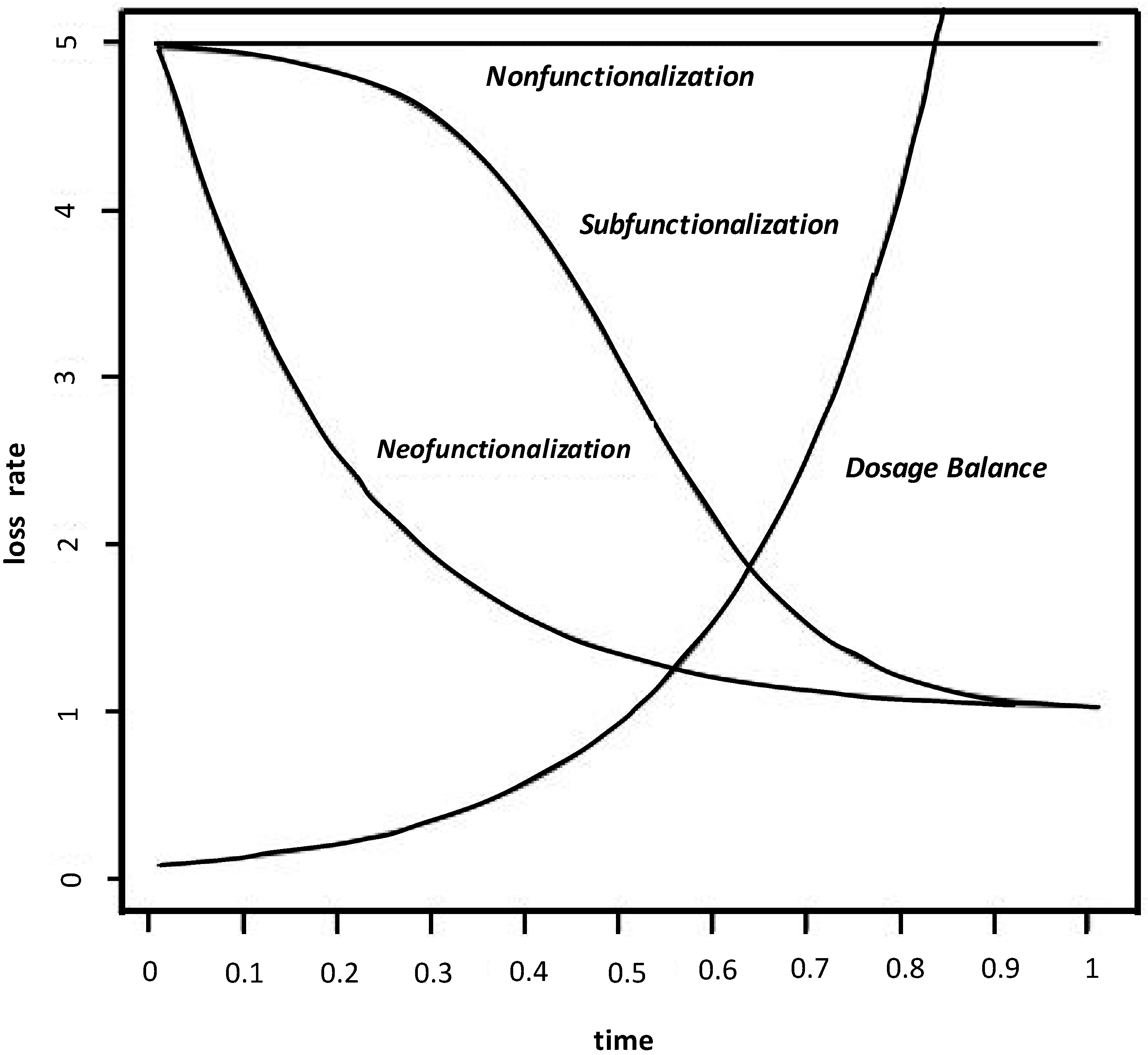
In extending the time heterogeneous gene retention model to a phylogenetic birth-death process, a simpler mathematical function than Equation (4) is desired. The instantaneous rates of loss under different gene fates are modeled here by a loss function associated with a generalized Weibull hazard function (
Figure 5), in which different sets of parameterization generate hazard curves indicative of different gene fates after a duplication event, mimicking those from Equation (3),
The parameters
u and
a are positive, while
b > 0 for subfunctionalization (
a > 1) or neofunctionalization (
a < 1),
b < 0 for dosage compensation and
b = 0 for nonfunctionalization. The constant
u must satisfy
u +
![Computation 02 00112 i004]()
> 0 when
b < 0, because the loss rate μ(
t) must be positive.
Figure 4.
(A) A scheme showing the transitions between different hazard rates based upon evolutionary processes is presented. Non-redundant and redundant hazard functions differ in that non-redundant genes are much less likely to be lost from a genome in any given time period. Neofunctionalization and subfunctionalization are processes that lead to the transition from a redundant rate to a non-redundant rate; (B) The same Markov process is described mathematically in terms of gene family size (n), sets of redundant genes (m), the duplication rate (c), the nonfunctionalization rate of redundant (a) and non-redundant (b) genes, the neofunctionalization rate (g) and the subfunctionalization rate (h(t)). In this formalization, αneo from (A) becomes g and αsub from (A) becomes h(t).
Figure 5.
The hazard functions associated with the nonfunctionalization, neofunctionalization (plus nonfunctionalization), subfunctionalization (plus nonfunctionalization) and dosage balance (plus nonfunctionalization) processes, as described by sample parameterization from Equation (7), are shown. Equation (3) generates a similar set of curve shapes. A version of this figure also appears in Liberles
et al. [
3].
The gene duplication/loss process is a non-homogeneous birth and death process with a time-dependent loss rate μ(
t) and a constant birth rate λ [
24]. With time since duplication, duplicates approach an asymptotic loss rate, and genes with no evidence of duplication are treated with a loss probability equivalent to this asymptotic rate that is parameterized as part of the model. The stochastic process of gene duplication and loss can be used to describe the evolutionary process of gene families within a single population. Let {
xi;
i = 1,…,
n} be the gene copies of a family at the present time (note that the model presented here refers to the evolution of copies within a gene family, as opposed to duplicate counts at a similar age in different gene families within a genome in the earlier part of the manuscript). Two gene copies
xi and
xj may have a common ancestor at time
t if a duplication event occurred at time
t and generated two copies that later evolved to copies
xi and
xj. The history of gene copies is represented by a gene family tree, which consists of two sets of parameters; a labeled history of gene copies {
xi;
i = 1,…,
n} and the node times {
ti;
i = 2,…,
n} with
t2 <
t3 < ∙∙∙ <
tn. The gene family tree follows a generalized birth process [
25] with a birth rate λ
P(
t,
z) in which
P(
t,
z) is the probability that a single lineage alive at time
t has some descendants at a later time
z [
26],
i.e.,
![Computation 02 00112 i005]()
, where
![Computation 02 00112 i006]()
. Thus, we have:
To calculate
P(
t,
z) in practice, we only need to solve the integral part in Equation (8). A derivation can be found as follows:
where
2F1 is a generalized hypergeometric function that can be calculated with an
R function, hypergeo [
27]. A gene family tree involves two types of events: duplication events and survival events (
n lineages are alive at the present time
T). Thus, the likelihood function of the duplication times {
ti;
i = 2,…,
n − 1} is the product of the likelihoods of duplication and survival events,
i.e., [
26].
Note that
![Computation 02 00112 i010]()
is the likelihood of (
n − 2) duplication events, and 1 −
w(
t) =
P(0,
t)
eρ(t,0) is the survival probability,
i.e., the probability that a lineage has exactly one progeny after an amount of time
t [
26]. Since there are
![Computation 02 00112 i011]()
labeled histories for gene copies {
xi;
i = 1,…,
n}, the likelihood function of a gene family tree
G is:
The likelihood function in (10) can be used to estimate model parameters, including the duplication rate λ and parameters (u, a, b) in the loss rate function µ(t) from gene family sequence data. Moreover, this likelihood function can be generalized to describe the evolutionary process of gene families within a species tree, where gene duplication and loss follow a non-homogeneous birth and death process occurring along the lineages of the species tree. The parameters, including the duplication and loss rates, can be estimated under this stochastic model.
Differentiation of loss and missing data or estimation of the species-lineage expectation of missing data will be necessary for the model to function properly. Additionally, the processes being modeled describe average processes and necessitate a large dataset of gene families to be simultaneously parameterized, with databases like The Adaptive Evolution Database (TAED) [
28] as an example. In such databases, tens of thousands of gene families from multiple species reflecting multiple duplication, loss and retention events per family can be evaluated together. In this type of analysis, it is envisioned that a mixture of parameterizations and mechanisms will be supported, with the number of independent parameterizations determined statistically. The support for each individual duplicate from each model/parameterization can also be evaluated probabilistically
a posteriori. This modeling framework is generalizable to related time homogeneous and time heterogeneous models.


 , where
  . Thus, we have:


 is the likelihood of (n − 2) duplication events, and 1 − w(t) = P(0,t)eρ(t,0) is the survival probability, i.e., the probability that a lineage has exactly one progeny after an amount of time t [26]. Since there are
  labeled histories for gene copies {xi; i = 1,…,n}, the likelihood function of a gene family tree G is:
