Article

Computational and Statistical Analyses of Insertional Polymorphic Endogenous Retroviruses in a Non-Model Organism

1
Department of Statistics, The Pennsylvania State University, University Park, PA 16802, USA
2
Institute of Molecular Genetics, Academy of Sciences of the Czech Republic, Videnska 1083, Prague, Czech Republic
3
Department of Computer Science and Engineering, The Pennsylvania State University, University Park, PA 16802, USA
4
Department of Biology, The Pennsylvania State University, University Park, PA 16802, USA
5
Department of Pathology, Johns Hopkins University, Baltimore, MD 21287, USA
6
Department of Biochemistry and Molecular Biology, Penn State College of Medicine, Hershey, PA 17033, USA
7
Department of Fish and Wildlife, 4034 Fairview Industrial Dr. S., Salem, OR 97302, USA
*
Author to whom correspondence should be addressed.
These authors contributed equally to this work.
Submission received: 5 August 2014 / Revised: 20 October 2014 / Accepted: 24 October 2014 / Published: 28 November 2014
(This article belongs to the Special Issue Genomes and Evolution: Computational Approaches)

Abstract

:
Endogenous retroviruses (ERVs) are a class of transposable elements found in all vertebrate genomes that contribute substantially to genomic functional and structural diversity. A host species acquires an ERV when an exogenous retrovirus infects a germ cell of an individual and becomes part of the genome inherited by viable progeny. ERVs that colonized ancestral lineages are fixed in contemporary species. However, in some extant species, ERV colonization is ongoing, which results in variation in ERV frequency in the population. To study the consequences of ERV colonization of a host genome, methods are needed to assign each ERV to a location in a species’ genome and determine which individuals have acquired each ERV by descent. Because well annotated reference genomes are not widely available for all species, de novo clustering approaches provide an alternative to reference mapping that are insensitive to differences between query and reference and that are amenable to mobile element studies in both model and non-model organisms. However, there is substantial uncertainty in both identifying ERV genomic position and assigning each unique ERV integration site to individuals in a population. We present an analysis suitable for detecting ERV integration sites in species without the need for a reference genome. Our approach is based on improved de novo clustering methods and statistical models that take the uncertainty of assignment into account and yield a probability matrix of shared ERV integration sites among individuals. We demonstrate that polymorphic integrations of a recently identified endogenous retrovirus in deer reflect contemporary relationships among individuals and populations.

1. Introduction

Transposable elements (TEs) comprise a significant proportion of all eukaryotic species’ genomes examined to date [1,2,3]. There are several classes of TE, including endogenous retroviruses (ERVs) and long interspersed nuclear elements (LINES), which replicate via an RNA intermediate. New acquisitions or mobilization of existing elements can result in variation in their number and genome location among species [4]. ERVs in particular can have profound impacts on host genome evolution and on host phenotype by altering host gene expression and by inducing structural variation in the host genome. Although many ERVs no longer have the ability to replicate, they continue to contribute to host gene regulation [5,6,7,8]. Further, their presence in the genome provides evidence of colonization events at specific points along the ancestral lineage leading to a contemporary species [9].
ERVs are derived from infectious retroviruses, which are well adapted to utilize host transcription and splicing machinery in a tissue-specific fashion. In humans, only the human ERV-K family (HERV-K) has retained the ability to mobilize in the genome. This leads to insertional polymorphism in the population, a situation in which some individuals have the HERV-K at a specific location in the genome while the site, called a preintegration site, in others is intact [10]. Each ERV is inherited by descent, thereby recording the ancestral lineage of the individuals in which it resides. However, because ERVs have the potential to impact genome structure and gene expression, they are not necessarily neutral markers. The presence of an ERV at a specific genome location in some individuals but not others provides the potential to confer phenotypic variation among individuals within or between populations. As genomes become available for more members of the tree of life, it is clear that an array of extant species have insertionally polymorphic ERVs due to either ongoing colonization or active retrotransposition [10,11,12,13]. To advance understanding of the role of ERVs on the evolution of their host species and on contemporary phenotypes, comprehensive approaches are needed to identify the population of ERVs in the genomes of model and non-model organisms.
We recently described an endogenous retrovirus (CrERV) that is a new Gammaretrovirus member [12] and has been colonizing its mule deer host (Odocoileus hemionus) since this species evolved from a common ancestor with white tailed deer (Odocoileus virginianus) about 1 million years ago [14,15]. As a result, there is extensive insertional polymorphism among individuals within and between populations. Some CrERVs are transcriptionally active in mule deer [12]. Under normal physiological conditions, it is presumed that most ERVs are transcriptionally silenced by the host [9,16] and that failure to do so is associated with disease [17,18,19,20,21]. It is, therefore, extraordinary to have an outbred population in which transcriptionally active ERVs and insertional polymorphism are the norm.
ERVs that have recently mobilized in or colonized a species are essentially identical and present challenges for accurate placement during genome assembly [22]. Even in the human genome, an expanding family of HERV-K, which resides in centromeric regions, was not identified until recently [23]. Methods that specifically detect host-virus junction fragments can be used to investigate ERV-host coevolution in any species. In the absence of a reference genome, de novo clustering of these fragments can be used to group the virus integration site derived from homologous host genome segments of different individuals [24]. However, with any method, there is uncertainty in assigning the status of an ERV in a host, caused in part by repetitive sequences present at the site of integration in the host and by the error rate of each sequencing platform. In particular, evidence that an individual carries a specific ERV is dependent on read count data; misinterpretation of these data leads to both false positives and false negatives.
The goals of this research were to develop a de novo approach to identify polymorphic integrations of ERVs and to account for uncertainty in ERV assignment to an individual. We apply a de novo clustering method to identify host-virus junction fragments without the use of a reference genome and develop a mixture model to estimate the uncertainty in ERV status. The resulting data are a matrix of probabilities for each ERV in each individual in the sampled populations. We demonstrate one application of these data to investigate the relatedness of Oregon blacktail deer (Odocoileus hemionus columbianus) and mule deer (Odocoileus hemionus hemionus) from both Oregon and Montana. The approach we present is applicable to any type of transposable element from model or non-model organisms and allows downstream analyses to be based on probabilities instead of a presence-absence status based on arbitrary thresholds of element read counts.

2. Experimental Section

2.1. Fluorescent In Situ Hybridization (FISH)

To generate the FISH probe, a full length CrERV sequence was amplified from mule deer genomic DNA by polymerase chain reaction (PCR) using primers: 5'-TCCCTTCCCCTATACCTGCT and 5'-CCAACCCTCTCTTTGGGTTT, and then subcloned into a pSC-A-amp/kan plasmid (Stratagene, La Jolla, CA, USA). The probe was directly labeled by nick translation with ChromaTide Alexa Fluor 594-5-dUTP (Invitrogen, Carlsbad, CA, USA) according to manufacturer’s protocol. Metaphase spreads were prepared and FISH performed as previously described [25,26]. DNA FISH slides were analyzed on Nikon TE2000-U microscope (Nikon Instruments Inc., Melville, NJ, USA) with a 60× objective and captured with Roper Scientific CCD camera (Roper Scientific, Trenton, NJ, USA) and NIS element software (Nikon Instruments Inc., Melville, NJ, USA).

2.2. Animal Samples

Animal tissues were collected at hunter check stations by state officials in Montana [MT] and Oregon [OR] from hunter killed animals and are exempt from IACUC review. The samples were obtained and processed as described [12]. The geographic location of these samples is indicated in Section 3.6. All animals were identified by morphology as belonging to mule deer (Odocoileus hemionus hemionus) or blacktail deer (Odocoileus hemionus columbianus).

2.3. Junction Fragment Analysis

The next generation sequencing libraries of CrERV integration sites were prepared by adapting previous methods for mobile element junction fragment analyses [27,28,29,30]. Briefly, the mule deer genomic DNA was digested with dsDNA fragmentase (New England Biolabs, Ipswich, MA, USA) to generate fragments in the 250–1000 bp range and purified with AMPure beads (Beckman Coulter, Brea, CA, USA). The resulting fragments were end-repaired and modified to create 3'A overhangs. DNA linkers were annealed and ligated to the end-repaired genomic DNA fragments. The linkers were designed with features that prevent linker-to-linker amplification of DNA fragments lacking the target retrovirus sequences. The sequences of the linker top strand is: 5'-GTGGCGGCCAGTATTCGTAGGAGGGCGCGTAGCATAGAAC*G*T (* denotes phosphorothioate bonds which prevent the degradation of the linker end). The sequence of the bottom strand is 5'-p-CGTTCTATGCTAC-N (p denotes 5' phosphate to enable ligation of the linker; N indicates the 3' amino modification used to prevent linker extension); both were obtained from Integrated DNA Technologies (Coralville, IA, USA). Approximately 150 ng of DNA with ligated linkers was then used as template in PCR amplification of the virus-host junction sequences (CrERV integration sites). PCR mixtures contained the following: 1.5 units of Ex Taq DNA polymerase (Clonetech Labs, Mountain View, CA, USA), the manufacturer’s reaction buffer, 0.2 mM dNTPs and 400 nM primers. The linker-specific primer was identical for all samples and contained the P1 adaptor sequence required for emulsion PCR and Ion Torrent amplicon sequencing. The sequence of the linker-specific primer is: 5'-CCTATCCCCTGTGTGCCTTGGCAGTCtcagGCGGCCAGTATTCGTAGG, where the underlined part is the P1 adaptor, TCAG in small letters is the key sequence used to calibrate the signal during the sequence run, and the remaining 3' end sequence is complementary to the linker. The long terminal repeat (LTR)-specific primer contains the A adaptor sequence required for emulsion PCR and Ion Torrent amplicon sequencing. For each sample, the primer contained a unique library-specific index or barcode of 5 or 8 nucleotides designed based on the Roche Multiplex Identifier (MID) sequences. The sequence of the LTR-specific primer is: 5'-CCATCTCATCCCTGCGTGTCTCCGACtcagxTCCTTCTTGCGTTTTGCATTGTCTC, where the underlined part is the A-adaptor, TCAG in small letters is the key sequence, x denotes the position of the barcode sequence and the remaining 3' end sequence is complementary to the CrERV LTR. Cycling conditions were: 95 °C for 2 min initial denaturation, followed by 28 cycles of 95 °C for 15 s, 60 °C for 25 s, 72 °C for 1 min, and then final extension of 72 °C for 5 min. The PCR products were size-selected by gel electrophoresis. The region corresponding to approximately 220–380 bp range was excised and purified from gel slices using QIAquick gel extraction kit (Qiagen, Valencia, CA, USA). A second size selection was done on the automated gel isolation system (Pippin Prep, Life Technologies, Grand Island, NY, USA) to narrow the size range to 300–330 bp that is optimal for Ion Torrent sequencing. The size profile and concentration was determined on the Bioanalyzer 2100 chip (Agilent, Santa Clara, CA, USA). All barcoded libraries were pooled and processed for sequencing on the Ion Personal Genome Machine (Life Technologies, Grand Island, NY, USA) using the Ion 318 chip.

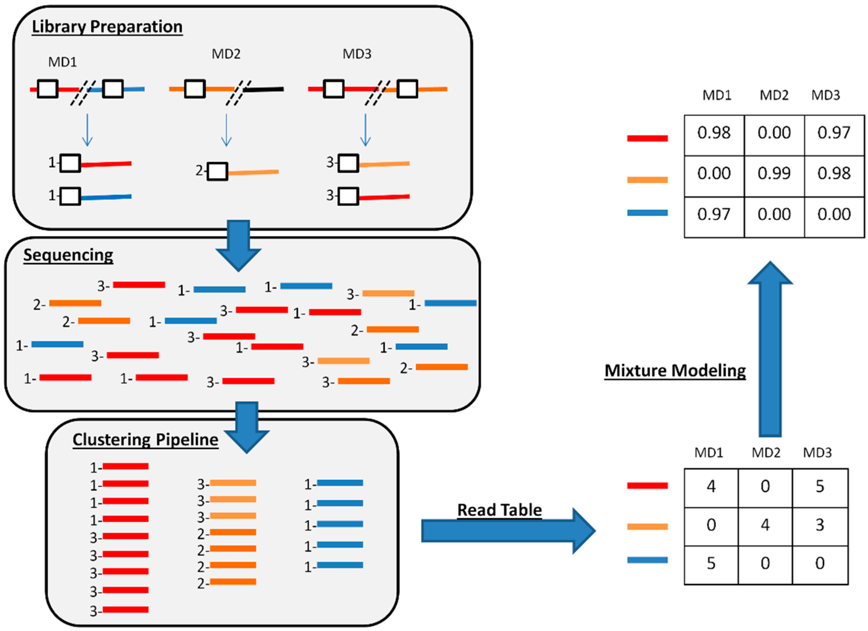
2.4. De Novo Clustering of Host-Virus Junction Fragments

The reads obtained from Ion Torrent sequencing were preprocessed by quality and length and the primer and adapter sequences in a read were removed. The sequences were selected to match the virus LTR that is common to those CrERVs that integrated within the last 200,000 years [31]. The reads were renamed according to their animal of origin and trimmed to 75 bp (containing 20–22 bp of LTR + 53–55 bp of the flanking host sequence) and clustered using the clustering pipeline previously described [32]. Briefly, reads are clustered using clustering software USearch (version 5.2.32 [33]) in two rounds. The clustering thresholds for optimal clustering of the reads are determined by varying clustering thresholds in 5% increments from 75%–95%. Internal compactness measures, the Dunn Index and Davies-Bouldin index, are used to determine the parameters that optimize clusters. For the experimental data the settings for the first round were 85% identity, gap open penalty: 2I, gap extension: 0.5, max accepts: 0, maxrejects: 0, ID definition: 1, user sort option. The clusters after first round that contain two reads or less are removed, and the consensus sequences of remaining clusters are again clustered at 90% identity in a second round of clustering using the same parameter settings.
All reads in the original data set are mapped to the consensus sequences of clusters obtained from the second round of clustering to obtain the number of reads per animal for each CrERV integration site. The mapping of reads was performed using USearch [33] with the following settings: query mapping to database option: global mapping, gap open: 2I, gap extension 0.5, ID definition: 1, user sort option, percent identity: 85%.
To ensure that each cluster corresponds to a single CrERV integration site, we compute inter-cluster distances between all pairs of clusters. All clusters with an inter-cluster distance less than 1.2 are merged using the linkage function for hierarchical clustering in Matlab software (Mathworks, Natick, MA, USA) and an in-house Perl script.

2.5. Mixture Model

Instead of taking an arbitrary cutoff value to determine whether CrERV i is carried by animal j, we address the uncertainty of CrERV status for small counts by a two-component mixture model (Poisson and truncated Geometric). The model assumes that when animal j carries CrERV i, the read count nij follows a Poisson distribution with mean λij:
P ( n i j = k ) = λ i j k e λ i j / k !             k = 0 , 1 , 2 ,
where λij = λi × λj and furthermore, when animal j does not carry CrERV i, the read count follows a truncated Geometric distribution with parameter 0 < p < 1:
P ( n i j = k ) = p ( 1 p ) k / [ 1 ( 1 p ) K + 1 ]             k = 0 , 1 , 2 , K
In Equation (1), we assume that λij = αi × βj where αi and βj are CrERV and animal specific parameters, respectively. In Equation (2), the geometric distribution is the discrete analogue of the exponential distribution where the probability mass function decreases with the number of false positive counts; we take K = 9, and the probability of a false positive may be found by 1 – P(nij = 0). The truncation means if at least K + 1, or 10, reads are observed, then the corresponding CrERV must be present according to our model. The likelihood of above mixture model is:
L ( α , β , p , π | n ) = Π i = 1 N Π j = 1 M ( π i f ( n i j | λ i j ) + ( 1 π i ) g ( n i j | p ) )
where N is the number of CrERVs, M is the number of animals, and πi is the mixing probability of the read count being generated from a Poisson distribution and can be interpreted as the prevalence of CrERV i among the N individuals. F(nijij) is the probability mass function of the Poisson distribution given in Equation (1) and g(nij|p) is the probability mass function of the truncated geometric distribution given in Equation (2). The parameter estimation can be carried out efficiently by a standard computational statistical tool known as the expectation-maximization algorithm [34].

2.6. Validation of Mixture Model via Replicated Individuals

The read counts come from two independent experiments, labeled the MT dataset and the S (which includes animals from both MT and OR) dataset, and 10 deer are sequenced in both experiments. If the CrERV status is accurate, then we would expect agreement between the results from the two experiments for the same deer; e.g., if CrERV i is positive in the MT dataset then it is also positive in the S dataset, and vice versa. Therefore, we can use the proportion of mismatched CrERV for each deer with replicates as a measure of CrERV status accuracy. We calculate this proportion for different cutoff values for the read count, ranging from 1 to 10, as well as for the mixture model with a cutoff probability 0.5.

2.7. Principal Component Analysis

We utilized principal component analysis to determine how the matrix of CrERV probabilities informed the relationships among the animals. For this purpose, we viewed each animal as a point in high-dimensional space, then use principal component (PC) to reduce this dimension to two. The original number of dimensions is the number of viruses. However, we eliminated viruses that were present in fewer than two animals, on the theory that such viruses provide no information about the relationship of pairs of animals. Thus, we considered principal components on the 1268 by 45 matrix resulting from removing all rows (CrERVs) present in only one animal.
After calculating the correlation matrix (a large square matrix of dimension 1268 by 1268) for the 45 column vectors of the probability matrix, the principal component analysis proceeds by identifying the eigenvectors corresponding to the largest two eigenvalues of the correlation matrix. These eigenvectors give the PC loadings, which may be dot-multiplied by a column of the original probability matrix to give that column’s PC scores. To determine how the PC scores relate to the geographic location of each animal, we matched the PC scores and locations as closely as possible using scalar multiples of each PC score followed by a rotation of the two-dimensional scaled PC scores.

2.8. Determine the Relationship of Animals via Ensemble Cluster

Kamath et al. [31] have used an ensemble cluster approach to successfully integrate the information carried by 12 CrERVs and to determine the relationship of mule deer. Let Y be an N by M binary matrix, where Yij = 1 indicates animal j carries CrERV i. Letting X = YTY be a consensus co-association matrix that integrates the clustering solutions inferred by multiple CrERV [35], we see Xij is the number of shared viruses between animals i and j. This approach can be extended by replacing the binary matrix Y by a probability matrix, Z, estimated from a mixture model, where Yij is the probability that individual j carries CrERV i.
One advantage of using the ensemble cluster method is that it allows us to put different weights on the CrERVs. These viruses have colonized the animals’ genomes over a 0.2 million year period up to the present [31]. The younger the virus being shared between a pair of animals, the stronger the relationship between the animals. Therefore, we assign a larger weight to the younger viruses in the consensus co-association matrix by letting X = YTWY, where W is an N by N diagonal matrix and Wj is the weight for the jth virus. We expect that CrERVs that have recently integrated into the genome will have a low prevalence in the population and take Wj to be inversely proportional to the estimated prevalence of CrERV j in the mixture model.
In addition to the observed co-associations, we assume the co-associations follow normal distributions under the null hypothesis that the presence of any CrERV is independent with the animal identification. We then calculate the expectation and variance of the number of shared CrERVs between each pair of animals under the null hypothesis, and consider the upper percentile of observed co-association as the p-value under the null hypothesis. The smaller the p-value, the more likely animals i and j are related.

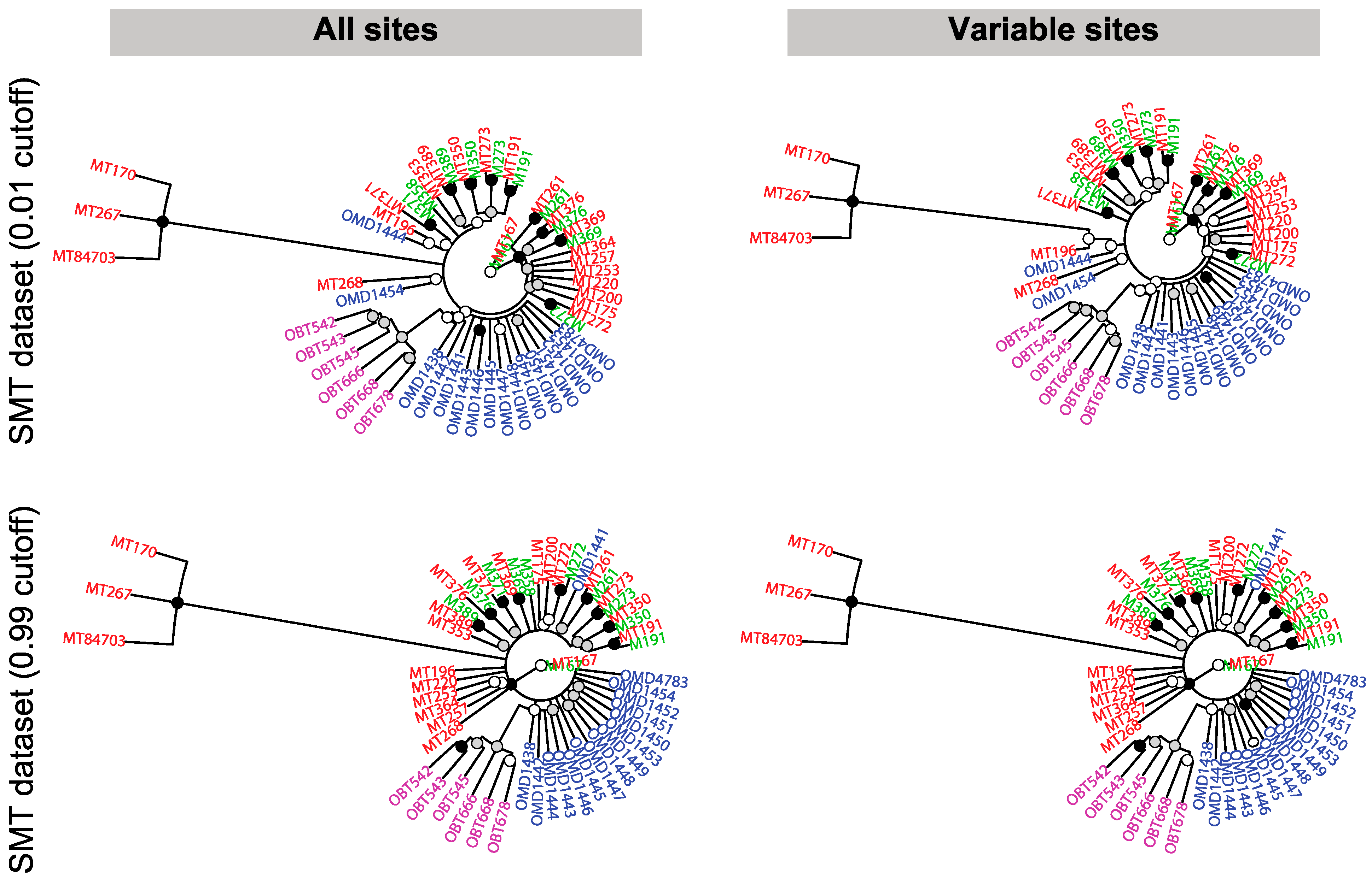
2.9. Visualization of Animal Relatedness by Hierarchical Clustering

To visually present the potential relationships among deer, we take the p-values for the test of independence as a distance metrics, and apply hierarchical clustering to the M by M distance matrix, where M is the number of animals.
The hierarchical cluster analysis merges small clusters into bigger ones sequentially using average linkage, starting from treating each individual as a unique cluster. The height in the dendrogram created by the hierarchical cluster analysis is the average p-value between two clusters (two child nodes).

2.10. Phylogenetic Analysis

Analysis of mule deer relatedness was performed with MrBayes. As input, using a probability cutoff of either 0.01 or 0.99, we created binary presence-absence data matrices from the probability matrix obtained from the mixture model. The MrBayes analysis was conducted using a setting with all sites or one with only variable sites. For each setting, we ran MrBayes using four chains for one million generations. A uniform prior was used for the tree topology, and we employed an unconstrained (non-clock) branch length prior from an exponential distribution with mean 10. Given a tree with topology and branch lengths, we used the Restriction Site (Binary) substitution model to model the presence-absence input data. We then constructed a consensus tree under each setting. These consensus trees were plotted using the ape package in R.

3. Results and Discussion

3.1. Overview of Research Objectives and Experimental Design

We recently described a new member of the Gammaretrovirus family (CrERV) that is colonizing its vertebrate host and is transcriptionally active. There is extensive polymorphism in populations for the presence or absence of CrERVs in mule deer, which provides an exceptional opportunity to investigate the coevolution of a free ranging mammalian host and a colonizing endogenous retrovirus. However, there is considerable uncertainty in high throughput sequence data that complicates interpretation of such data. We therefore developed an analysis platform suitable to investigate insertional polymorphism of ERVs in both model and non-model organisms. An overview of our workflow is shown in Figure 1.

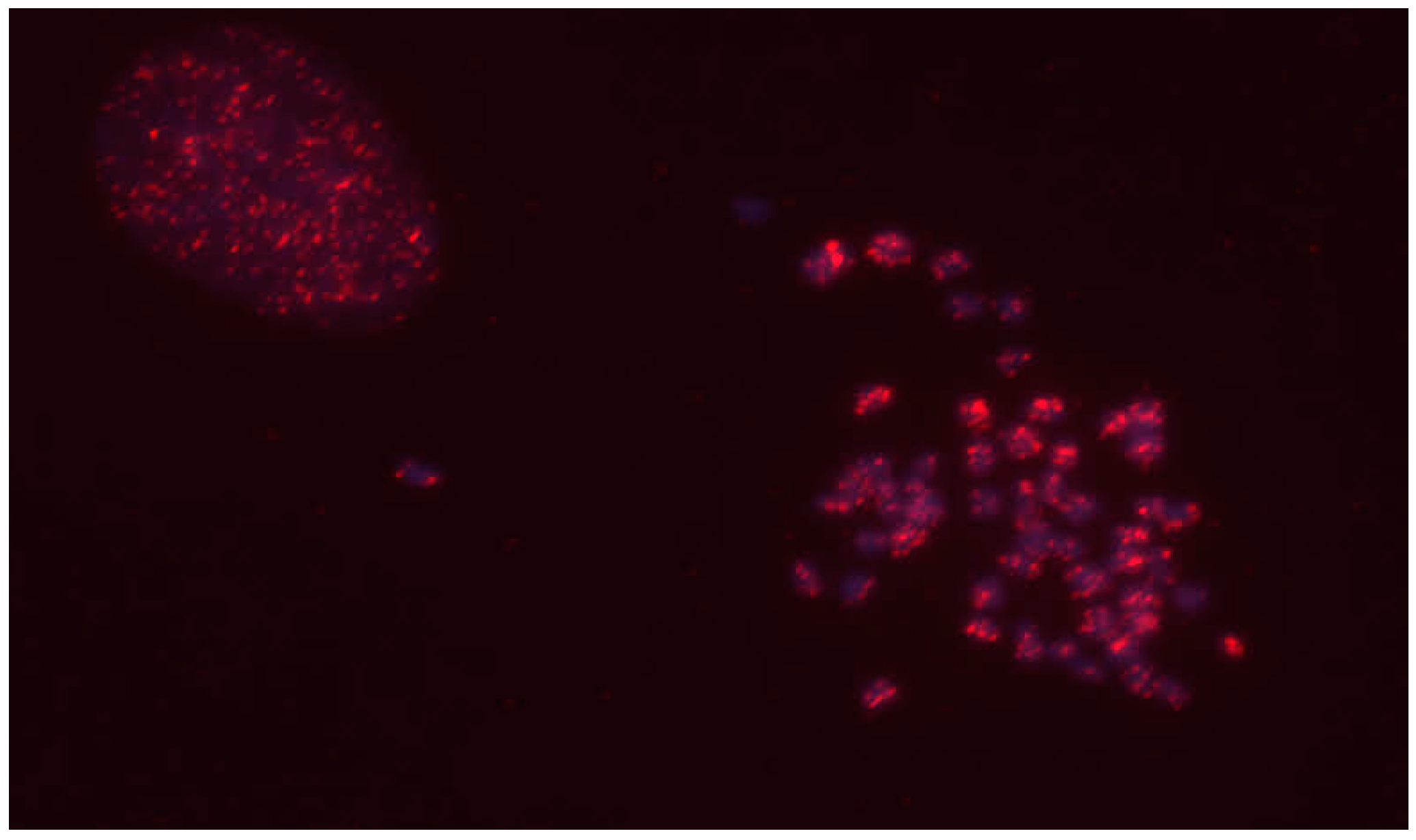
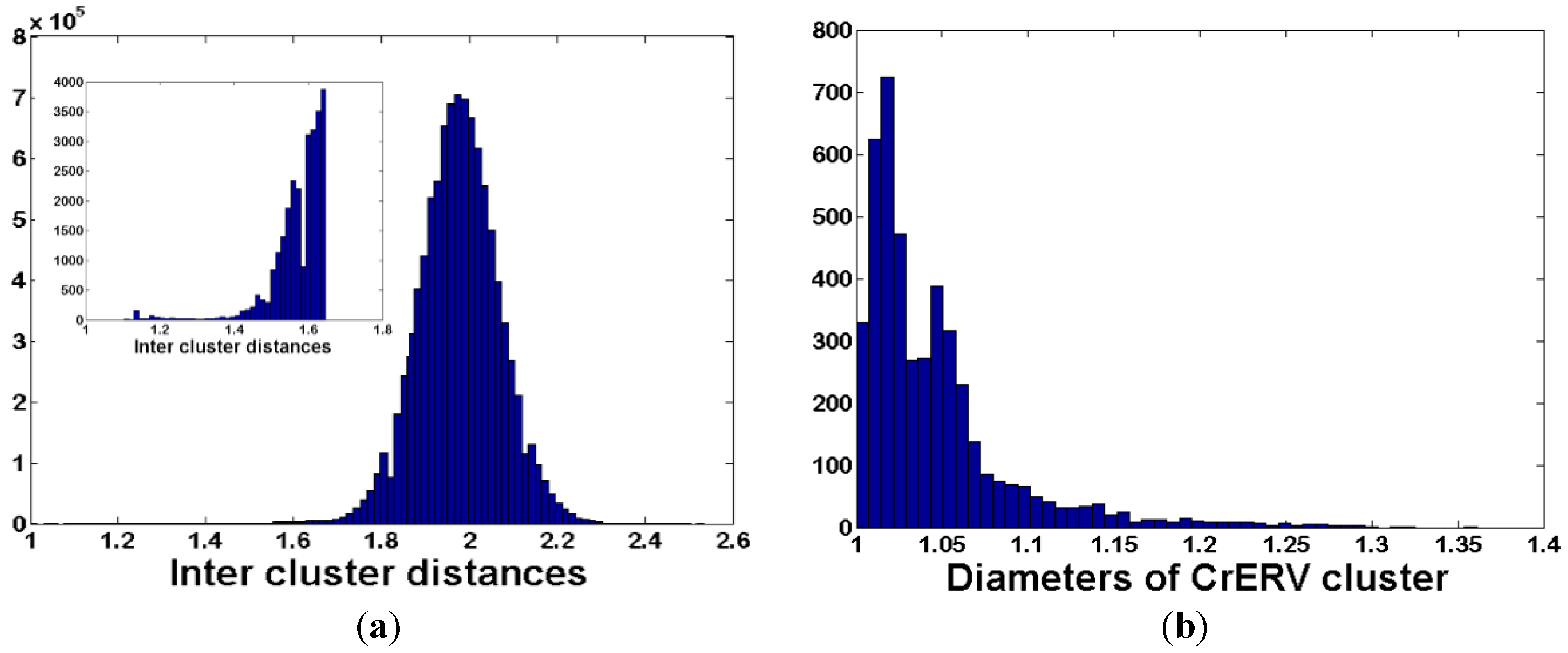
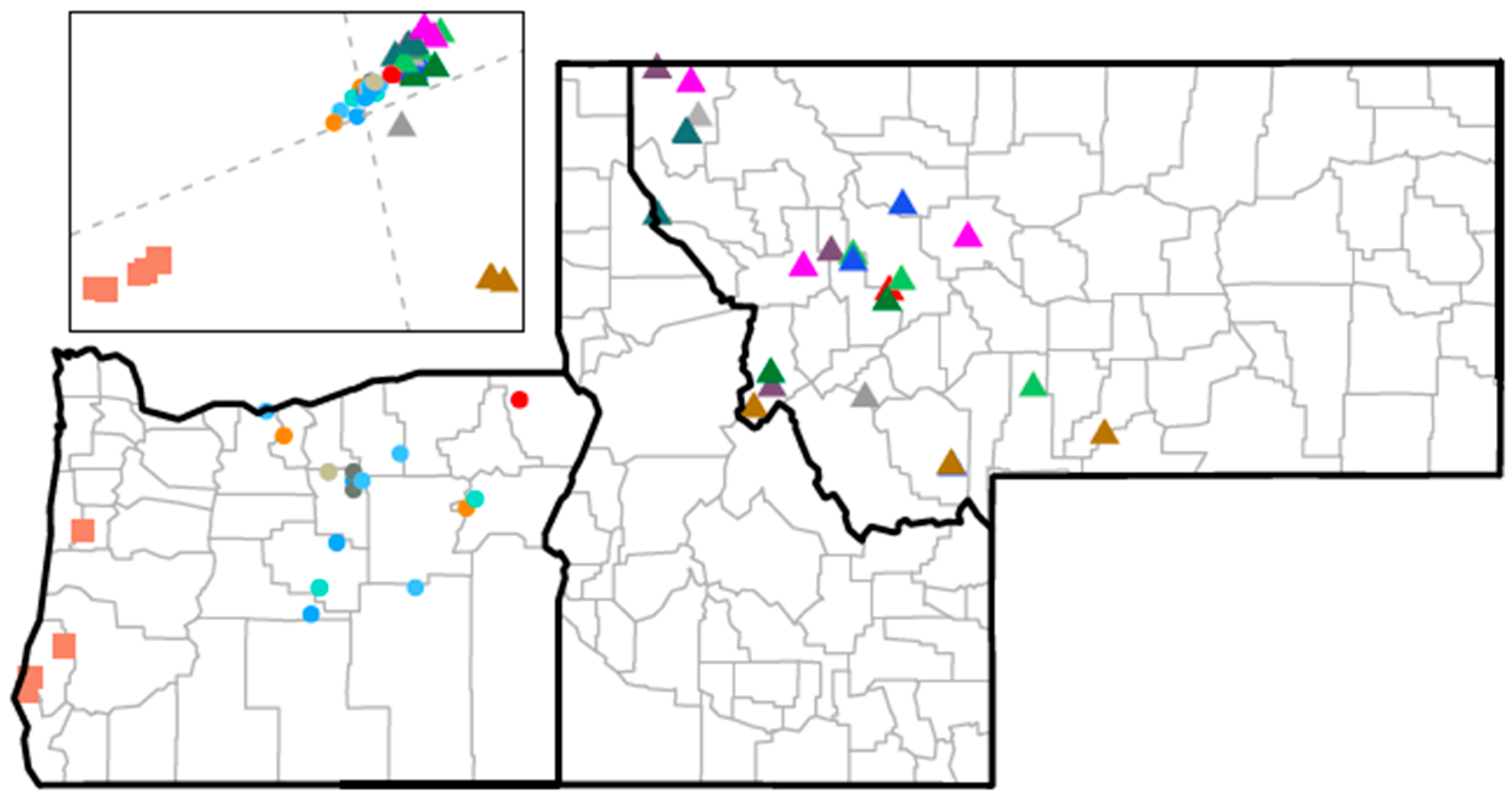
3.2. Fluorescent In Situ Hybridization Analysis of CrERV Locations

Because there are few genomic resources available for mule deer, we utilized de novo methods in lieu of reference mapping approaches to identify common insertion sites among animals. However, we previously demonstrated using simulated genomic data that integration sites localized in repeat regions affect the accuracy of de novo clustering of virus-host junction fragments [32]. We therefore evaluated the chromosomal distribution of CrERVs by fluorescent in situ hybridization (FISH) using a fibroblast cell line established from mule deer [36]. The data show that CrERV integration sites appear to be well dispersed among chromosomes and that they do not aggregate near centromeres or telomeres (Figure 2), which are enriched in repeat regions.

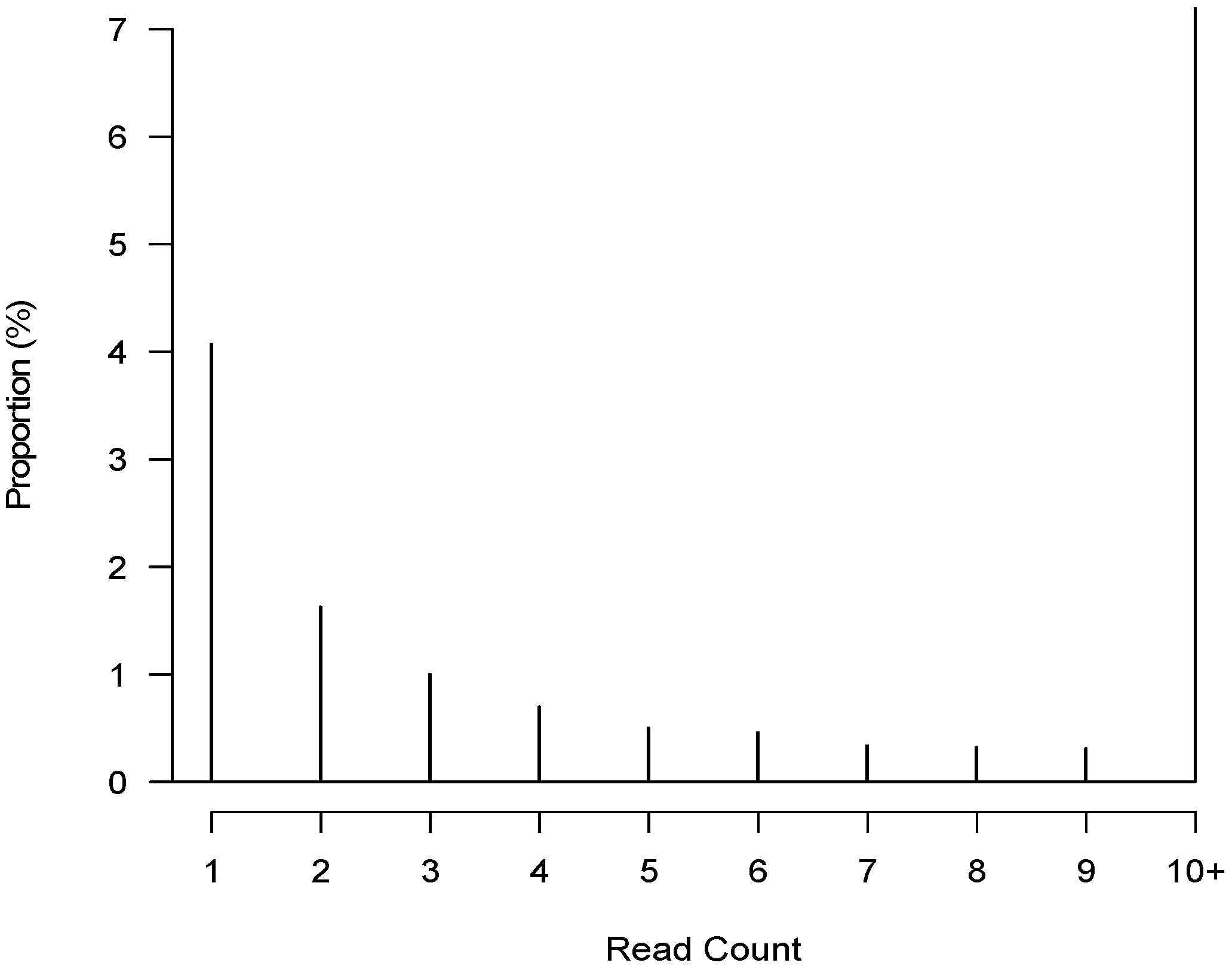
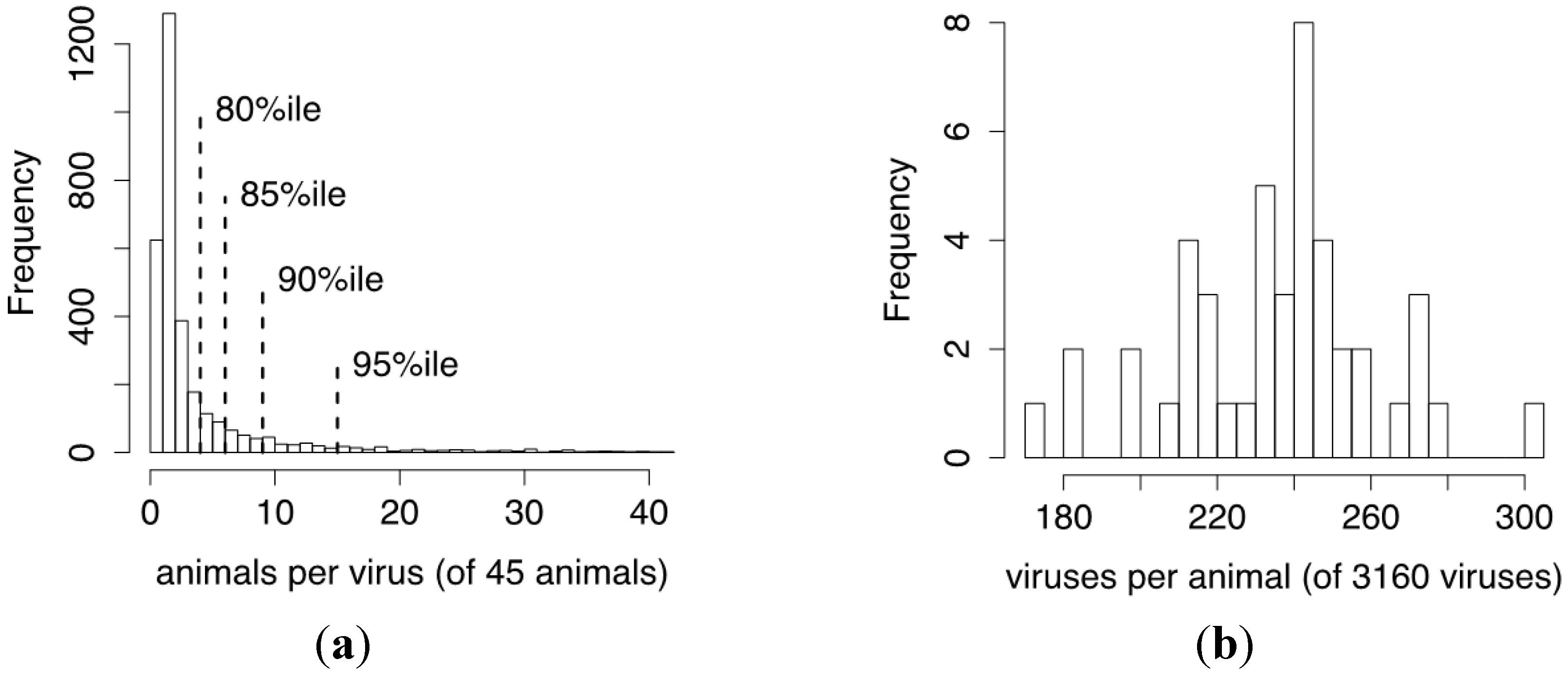
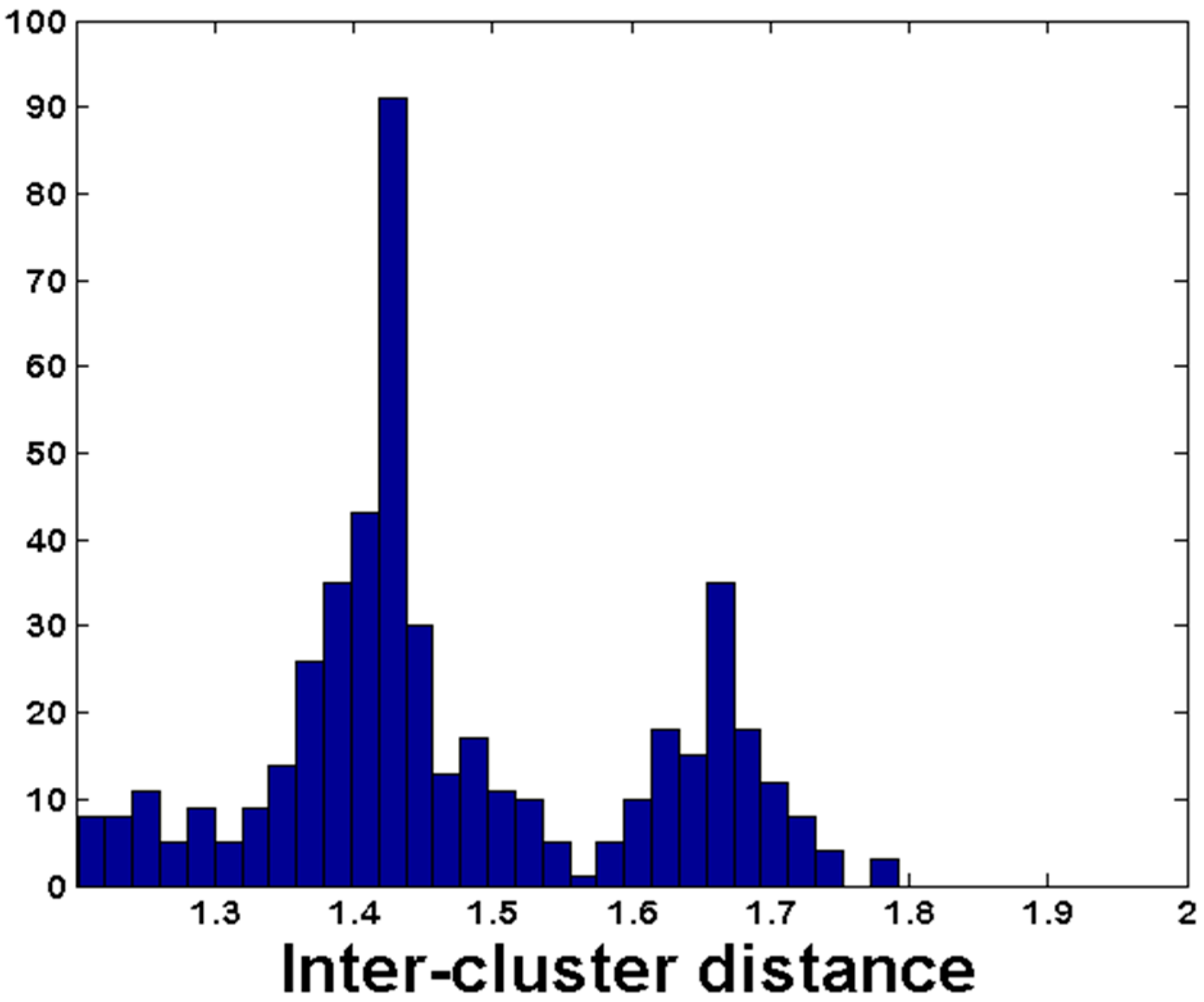
3.3. De Novo Clustering Analyses of CrERV-Host Junction Fragments

The goal of the clustering portion of our workflow is to group short sequence reads obtained from identical host junction fragments in our pooled libraries and to determine the number of reads from each animal that is assigned to the cluster (Figure 1). To obtain the sequence data, we modified a high throughput approach for cataloging mobile elements [27,28,29,30] to identify CrERV integration sites in individual animals. Libraries are prepared by enriching the host sequence flanking the 3' end of a CrERV integration and are sequenced using Ion Torrent technology. Our final data consist of a 20 bp fragment of the 3' CrERV LTR and a minimum of 45 bp of the host flanking sequence.
Figure 1. A schematic diagram of the workflow. For illustration purposes, three different CrERV integration sites, indicated by red, orange and blue colors, are shown from three different animals (marked MD1, 2 and 3). The CrERV-host junction fragment is enriched by PCR from the DNA of each animal and libraries are prepared, and then pooled and sequenced on the Ion Torrent platform. This results in a dataset of reads from all the CrERV-host junction fragments. These reads are clustered using the clustering pipeline to obtain three clusters representing the red, orange, and blue host genomic regions. Reads in a cluster are then separated into their animals of origin to obtain a read table. The read table is processed using mixture modeling to obtain the probability of correct assignment of each CrERV-host junction fragment clusters to each animal in the sample. In actual sequence data with higher read counts, low probabilities would reflect a spurious assignment of a read for a specific CrERV to an animal.
Computation 02 00221 g001
Figure 2. Fluorescent in situ hybridization of genomic distribution of CrERV integrations. Two nuclei of the mule deer cell line [36] are shown, one interphase (left) and the other in metaphase (right). The signal from Alexa Fluor 594 labeled CrERV probe is shown in red, the 4',6-diamidino-2-phenylindole (DAPI)-stained chromosomal DNA in blue. CrERV integration sites appear distributed along each chromosome.
Computation 02 00221 g002
Sequencing errors from next generation sequencing platforms and genomic repeat regions are major hurdles to accurate de novo clustering. The accuracy of de novo clustering is in part dependent on identity thresholds, which determine which sequences will be added to each cluster. We demonstrated with simulated data that empirically determining clustering thresholds from the data and using two rounds of de novo clustering significantly improved results [32]. In addition, we imposed statistical measures of intra-cluster compactness and inter-cluster separation (Dunn Index and Davies-Bouldin Index) to identify the optimized clustering parameters. The Dunn Index is the ratio of the minimum inter-cluster distance to the maximum cluster diameter; this value should be large if all clusters have small diameters and large inter-cluster distances [37]. The Dunn Index is sensitive to outliers and values should be greater than one. The Davies-Bouldin Index (DB index) is the averaged ratio of intra-cluster distance to inter-cluster distance, which will be small if all clusters are compact and have large inter-cluster distances [38].
We optimized clustering parameters for our experimental data by varying clustering threshold values in steps of 5% from 70% to 95% in each of two clustering rounds in UCLUST (a clustering option in USEARCH software; [33]). Based on the Dunn and DB indices, optimized clustering parameters were 85% and 90% for the first and second clustering rounds, respectively. The distribution of pairwise distances for the dataset demonstrates that the clusters are well separated from one another, with a small number of clusters having inter-cluster distance less than 1.2 (Figure 3a). These were merged in the final data set because they represent sequence reads from the same genomic location that were erroneously split into two clusters. The majority of clusters are compact, having diameters of less than 1.1 (Figure 3b), although clusters with diameters up to 1.4 are evident. All original reads are mapped back to the cluster consensus to yield the number of reads obtained from libraries of each animal for each unique CrERV-host integration site. We identified 3160 unique CrERV integration sites for this sample of 55 samples from 45 animals from Oregon and Montana. These data are compiled into a 3160 CrERV by 55 animal matrix for subsequent analysis.

3.4. Estimating the Probability of a CrERV Assignment Using a Mixture Model

The misinterpretation of read count data can result in failure to detect an ERV integration that is present or falsely assigning one to an individual when it is absent. Although a threshold approach is commonly used in practice, it has several limitations: (i) the uncertainty of ERV status is not taken into account when the count data is transformed to the binary ERV status data; (ii) the virus status implied by small count is sensitive to the threshold, but the choice of threshold value is often arbitrary; (iii) the same threshold would be applied to all read counts without controlling either the total read count per ERV or the total read count per individual.
The number of sequence reads assigned to a CrERV integration site for any animal can be affected by factors ranging from quality of the original DNA sample to technical issues in sequencing. These can result in differences in the total number of reads for each animal. Our data are derived from two separate Ion Torrent sequencing runs and there is substantial variation in the total reads, and consequently the average of non-zero read count of sequences representing CrERV integration sites, in each animal (range: 4.6–230, Figure 4a). Similarly, the number of sequence reads assigned to each CrERV integration site depends on genome position, whether the integration is homozygous or heterozygous, and technical factors related to library preparation and sequencing. This leads to a large variance in the average non-zero read count for each CrERV integration site (range: 1–1000, Figure 4b).
Figure 3. Features of clusters representing CrERV-host junction fragments obtained by de novo clustering. (a) Frequency distribution of inter-cluster distances. The x-axis is a measure of the pairwise distance between clusters and the y-axis represents the frequency of all pairwise distances for the data set of 3160 cluster consensus sequences. The pairwise distance among clusters will be small if clusters are derived from closely related sequences, e.g., from a similar repeat region, or if two sets of reads from different regions are merged. The peak in the frequency distribution near 2 in our data indicates that the sequences returned by our clustering are well separated. Inset shows an expanded scale for inter-cluster distances between 1.1 and 1.65. The threshold for combining closely related clusters was chosen as 1.2; (b) Frequency distribution of cluster diameters. The y-axis represents the frequency that a cluster diameter is observed and the x-axis represents cluster diameters, which are computed as the average distance of each read assigned to the cluster to the cluster consensus sequence. The majority of clusters have value close to one, indicating near perfect identity of individual reads in the cluster to the consensus sequence.
Computation 02 00221 g003
The distribution of read counts per animal in our data also shows that 4.7% of counts are values between one and nine (Figure 5). To address the uncertainty of CrERV status for small counts, we employed a two-component statistical mixture model under the following assumptions: counts for truly absent CrERVs are random and follow a truncated Geometric distribution with an upper bound of nine that is the same for each animal and CrERV, whereas counts for truly present CrERVs follow non-identical Poisson distributions. The results are a matrix estimating the probability of presence of each CrERV in each animal as well as estimated model parameters. Among the parameters, the estimated p of 0.925 for the truncated Geometric distribution yields a false positive probability of 0.075.
Figure 4. Distribution of reads assigned to CrERV. (a) The frequency distribution of the average number of sequences assigned to CrERVs assigned to each of the 55 animals, which includes 10 replicate animals. Variation in read count can occur because of differences in sample preparation, pooling, and between individual sequencing runs. The data show that there is, on average, a read count of 50 for CrERVs from most animals, but two animals have an average of over 200 reads per CrERV; (b) The frequency distribution of non-zero read count for the 3160 CrERV. The majority of CrERV integration sites are represented by a read count of between 1 and 100 but four CrERVs have over 850 reads.
Computation 02 00221 g004
Figure 5. Distribution of non-zero read count less than 10 for each CrERV. The histogram shows the proportion of the 3160 CrERV integration sites in 55 animals that have read counts from one to nine.
Computation 02 00221 g005
Our data consist of two independent sequencing runs and include two replicates of ten of the animals. If CrERV status were accurate, then we would expect agreement between the results from the two sequencing runs for the same deer. We calculate the classification error for different threshold values of read counts between one and ten, and for the mixture model where probability greater than 0.5 is taken to imply presence (Table 1). The threshold value that minimizes the differences varies from two to ten among the replicated animals, indicating that a single threshold would not decrease uncertainty in CrERV assignment. In contrast, the mixture model performs well in all animals. Because of the strong agreement within replicate animal pairs, we merged each replicate pair using the larger probability of each CrERV, yielding a single representative of each animal and a final data set of 45 individuals.
Table 1. The proportion of mismatched CrERV between two replicates for 10 animals. The data depict the number of mismatches at read count thresholds for 1–10 and for the mixture model. The read count threshold that minimizes the difference between replicates is in bold.
Animal ID12345678910Mixture Model
M1910.0830.0480.0390.0440.050.0530.0590.0650.0680.0760.049
M3890.1740.1010.0670.0470.0380.0330.0340.0340.0370.0340.034
M3500.1960.1060.0610.0410.0350.0340.0290.0290.0270.0250.025
M2610.0610.0320.0330.0330.040.0390.040.0430.0420.0410.033
M3690.110.040.0270.0250.0280.0270.0260.0210.0230.0240.028
M1670.1570.0790.0530.0470.040.0350.0350.0340.0350.0350.047
M3710.2080.0940.0570.0470.0410.0370.0350.0340.0380.0390.051
M3760.070.0550.060.0640.0660.0710.0720.0750.080.0810.062
M2720.2490.1270.0770.0640.0610.0590.0560.060.0630.0640.038
M2730.1030.0570.0420.0340.0300.0270.0280.0300.0280.0270.027
The accuracy of the mixture model estimates based on the read counts was assessed for five CrERV integration sites in 55 animals (including replicates) by PCR, or 275 sites overall. The 208 CrERV integrations confirmed to be absent by PCR all had estimated probabilities less than 0.01; thus, there were no clear false positives. On the other hand, four integration sites (with small read counts of one, one, three and six) were confirmed to be present by PCR despite very low (smaller than 0.0004) estimated probabilities. This yields a false negative rate of 4/67, or 6.0%.

3.5. CrERV Distribution in Mule Deer

The distribution of CrERVs shared among 45 individuals supports that there is extensive insertional polymorphism of CrERVs in mule deer (Figure 6a). More than 50% of CrERVs are found in only a single animal. Only 5% are found in more than 15 animals and none is found in all animals in the sampled populations. Each individual animal has between 180 and 280 expected unique CrERV integrations (Figure 6b), which is consistent with our empirical estimates [12]. The number of CrERV integrations does not differ between mule deer and blacktail deer.
We note that 15% of CrERVs had a probability of 10−6 or less of correct assignment to any animal. The histogram of pairwise distance of cluster sequences from these low probability CrERVs to all CrERVs is bimodal with peaks near 1.4 and 1.7 (Figure 7). The CrERV integration site sequences represented by the second peak are likely unique sequences based on the large pairwise distance between them and all other identified CrERV integration sites.
The overall relationship among animals based on the model-predicted number of CrERV assignments in common for all pairs of mule deer, including the replicates, can be seen in a heatmap (Figure 8). The replicate animals are easily identified as the ten larger squares along the diagonal. Two groups of animals that are closely related to each other but differ from other animals in CrERV composition are evident in the bottom right corner of the heatmap. One is a group of three Montana mule deer and the second comprises all the Oregon blacktail deer (O. hemionus columbianus). As mule deer and blacktail deer diverged about 22,000 years ago [39], the unique composition of CrERV in blacktail deer could be due to new colonization events or retention of an older lineage that was not passed on as mule deer diversified.
Figure 6. CrERV prevalence among animals and the number of CrERV integrations sites per animal estimated from the mixture model. (a) A histogram of the total expected number of animals in which a CrERV insertion site was identified according to the mixture model after merging the replicate animals. These data are derived as the sum of probabilities for each of the 3160 CrERV in the 45 animals. Various percentiles of the distribution are shown by dotted lines; the median number of animals in which any CrERV is found is 1.01 and only 5% of animals share 15 or more CrERVs; (b) The estimated number of CrERVs for each of the 45 animals is calculated by summing all probabilities of a CrERV integration for each animal. The horizontal axis gives the range of values, and the height of the corresponding bar gives the number of animals in that range. These data demonstrate that the majority of animals have between 200 and 280 CrERV integrations.
Computation 02 00221 g006
Figure 7. Inter-cluster distance for CrERVs with low probability of assignment to any animal. The histogram shows the frequency distribution of pairwise distances for cluster sequences representing the subset of 479 CrERVs with an estimated probability of correct assignment less than 10−6.
Computation 02 00221 g007
Figure 8. The heatmap depicts the entries in a square matrix in which the (i, j) entry is the number of CrERV assignments in common, as predicted by the mixture model, for animals i and j. Entries along the diagonal are the number of predicted CrERVs total for each animal. Darker (redder) colors indicate larger values, and the rows and columns are sorted automatically by the plotting function so as to keep similar columns close together. A total of 55 animals, including the replicates, are shown.
Computation 02 00221 g008

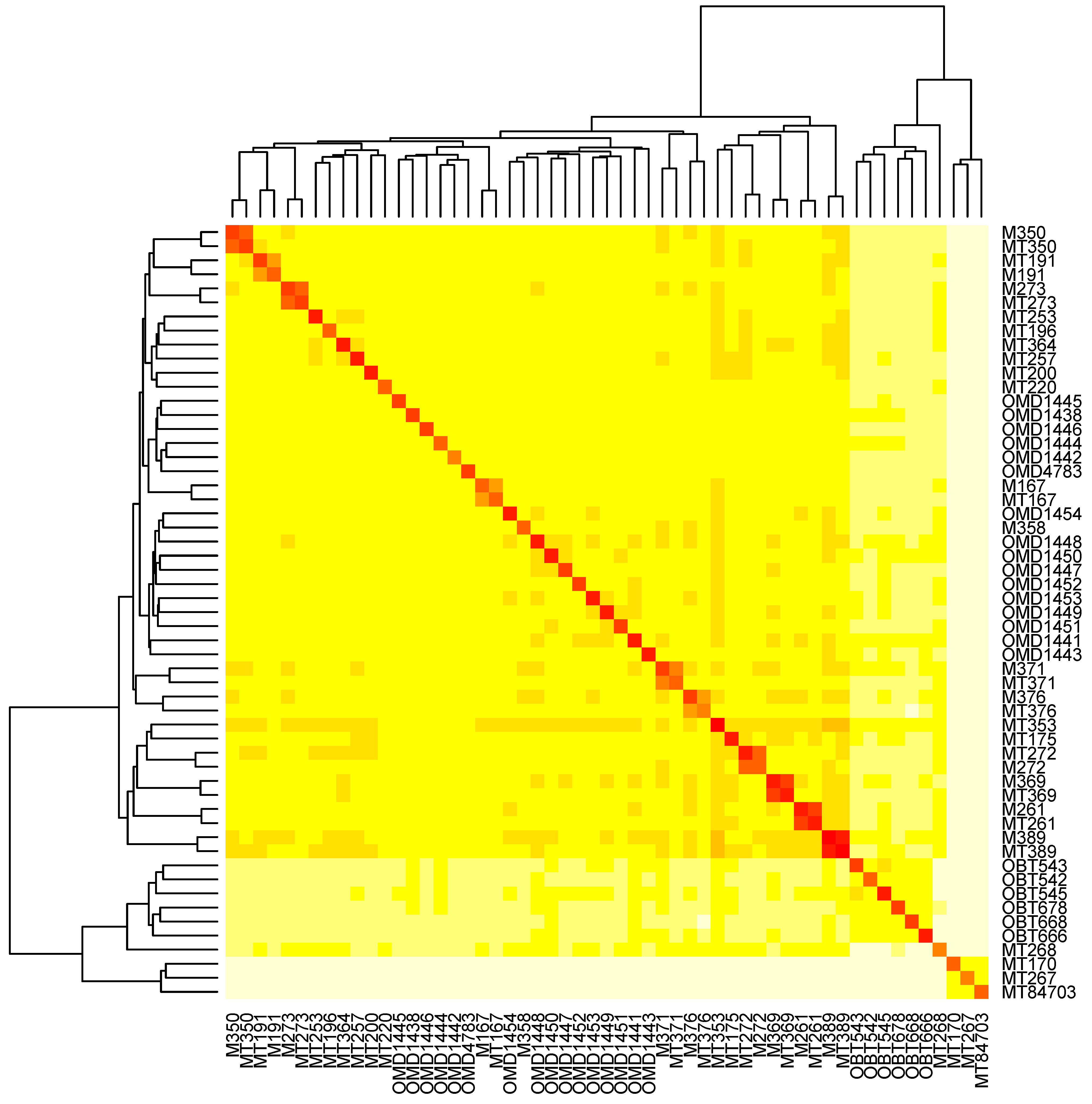
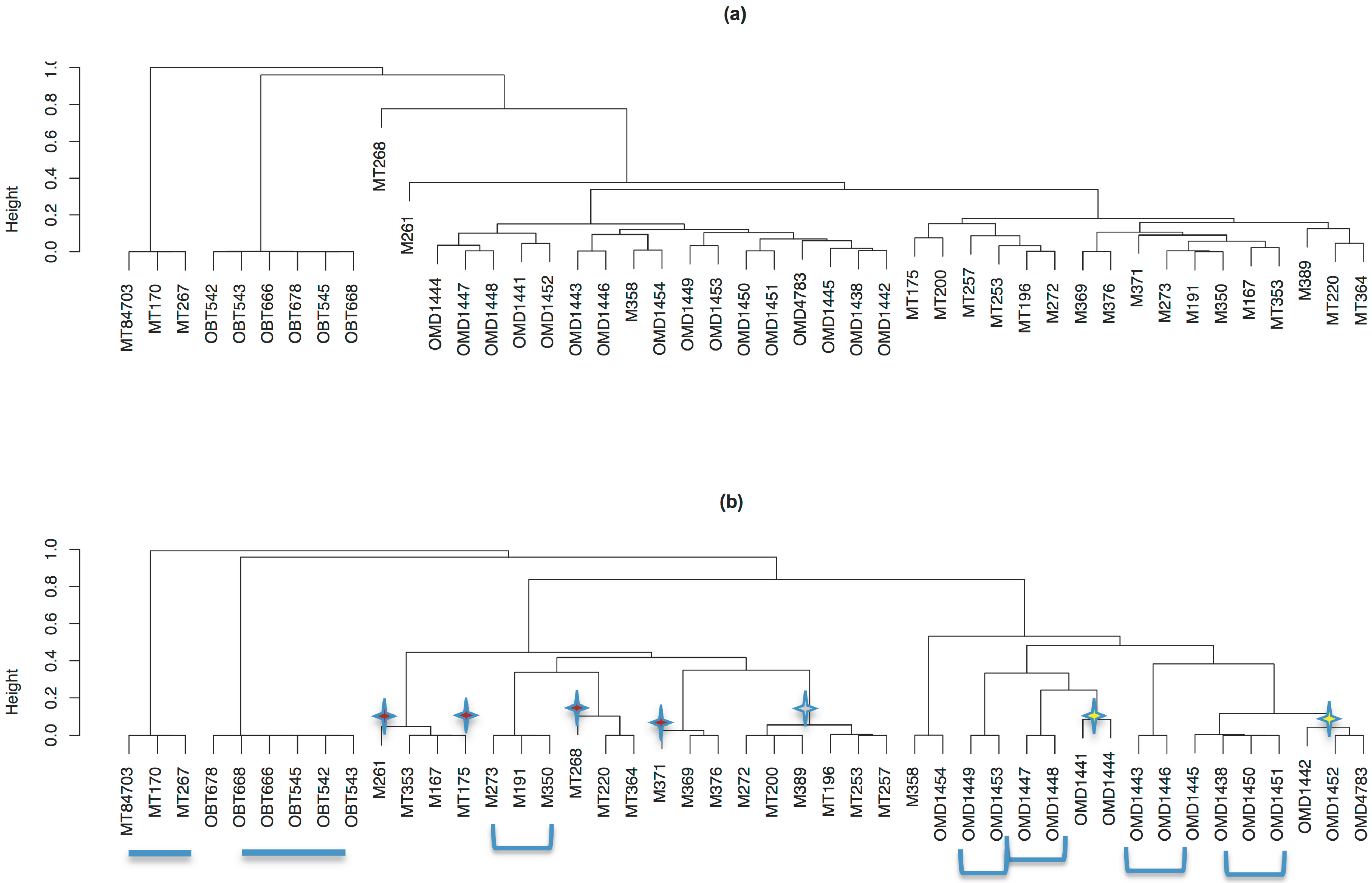
3.6. The Relatedness of Mule Deer Based on Shared CrERVs

The shared history of CrERVs among mule deer provides a means to trace the ancestral history of animals because two individuals can only share a CrERV by descent. Thus, it follows that animals with more shared CrERVs are more closely related. We previously utilized ensemble clustering to estimate relationships of 258 animals from a data set of 12 empirically determined CrERV integration sites [31]. Ensemble clustering produces a consensus co-association matrix that integrates the clustering solutions inferred from multiple CrERVs [35]. It also allows us to weight CrERVs that are present at low frequency in the population under the assumption that low-frequency viruses are likely to be younger, and the younger the virus being shared, the stronger the relationship between host animals. The data are visualized using hierarchical clustering (Figure 9).
Figure 9. Hierarchical clustering results of ensemble cluster data depicting relatedness of animals. (a) All CrERVs contribute equally; (b) low-frequency CrERV are weighted to increase their contribution. The depth of the branch indicates the p-value of two animals carrying CrERVs independently. The replicate animals are merged in this analysis, which is based on 45 animals. Blue underlines indicate the two outlier groups shown also in Figure 8 and Figure 10. Stars indicate the animals that change positions when low-frequency CrERV are weighted (red centers are Montana deer, yellow centers are Oregon deer. The gray centered cluster has gained support and repositioned three animals when weighting of low-frequency CrERVs is imposed. Blue brackets indicate those animal groups also supported by phylogenetic analysis shown in Figure 10.
Computation 02 00221 g009
Figure 10. Unrooted consensus population trees obtained from MrBayes using different probability cutoffs. The top and bottom rows represent a probability cutoff for the presence of a CrERV of 0.01 and 0.99, respectively. The left and right columns represent the full dataset and a reduced dataset of only loci polymorphic for a CrERV, respectively. The analysis is based on the complete data set of 55 animals, which includes the 10 replicates. Oregon mule deer are shown in blue, Montana mule deer in red, replicate Montana mule deer in green, and Oregon black tail deer in magenta. Nodes have the following colors: Black: ≥ 0.95 posterior; Gray: ≥ 0.75 and < 0.95 posterior; White: < 0.75 posterior.
Computation 02 00221 g010
There are several important features of mule deer relationships from these analyses. First, the Montana and Oregon mule deer populations form distinct groups. This separation is most evident when lower-frequency CrERVs are weighted but is also apparent without weighting. Blacktail deer and an outlier group comprised of three Montana deer form distinct lineages separate from the main mule deer groups, consistent with data in Figure 8. These three mule deer could represent mule deer–white tail deer hybrids or a divergent population of Montana mule deer, possibly immigrants from genetically divergent populations to the south. Animal MT358 is the only Montana deer sharing ancestry with an Oregon deer (OR1454). Increasing weight of low-frequency CrERVs places these two animals as an outgroup to the Oregon mule deer cluster. The relationships of seven Montana deer and five Oregon mule deer are affected by weighting.
We also evaluate relationships among deer using MrBayes by converting the probability matrix to presence–absence based on a cutoff of either 0.01 or 0.99 (Figure 10). The four main groups—Oregon mule deer, Montana mule deer, Oregon blacktail deer, and the outlier group of three Montana deer—are also evident in the Bayesian phylogeny. In addition, there is support for two sister groups of blacktail deer not seen in Figure 9. Where there is support for relatedness among mule deer, it is concordant with the hierarchical clustering data (Figure 9). Notably MrBayes results are sensitive to the threshold chosen for inclusion of CrERV sites; limiting the analysis to those CrERV with a probability of 99% or greater of being correct alters both the support and placement of animals in the phylogeny (compare OMD1441, 1444 and 1454 in Figure 10).
The geographic location of all animals and their relatedness estimated by hierarchical clustering are shown in Figure 11. The inset displays a principal component analysis, which further confirms the group separation defined by ensemble cluster and phylogenetic methods.
Figure 11. Map displaying geographical location and relatedness of animals. Points on the map give locations of the samples taken from the 45 animals. Squares denote blacktail deer; triangles and circles are mule deer sampled in Montana and Oregon, respectively. Points of the same color represent related groups of two to six animals shown in the bottom dendrogram of Figure 9. Inset displays the first two (scaled) principal component scores, after rotation indicated by the dotted gray PC score axes, derived from the 1268 × 1268 correlation matrix of the vectors of mixture-model estimated probabilities for the 1268 viruses present in at least two animals.
Computation 02 00221 g011

3.7. Discussion

High-throughput sequencing approaches permit extensive interrogation of genome variation in populations of individuals. Variation in the composition of mobile elements, such as ERVs, is one type of genome variation that can be determined in the absence of a reference genome. Because ERVs have the potential to exert a large effect on the host, their similarities and differences among individuals should be considered in studies of genomic associations with phenotype. As with any method relying on new sequencing technology, there are substantial sources of error that can complicate analyses based on shared genomic traits [40,41,42,43,44]. Our research provides an approach to incorporate the uncertainty in assigning a trait, in our case an ERV, to an individual.
Our approach does not employ a reference genome. Approaches that map reads to a reference can be affected by repeat regions, poorly annotated or absent regions in the reference build, and structural variation in the query compared to the reference genome. Any of these mapping problems can affect the number of sequenced reads that are assigned to a location. A large range in the distribution of read counts, with an abundance of single reads such as we report, is also obtained for TE insertion analysis in humans [27], which arguably is the best annotated genome available. Our approach using de novo clustering avoids problems associated with genome quality, because it does not require a reference genome. Yet clustering approaches have their own source of error. While we provide methods to optimize clustering parameters based on statistical measures and assess our results by determining how well resulting clusters are separated from each other, there are still errors in the cluster sequences representing the putative host genomic site of ERV integration; this affects the number of reads assigned to the cluster. Thus both mapping and de novo approaches suffer from the problem of how to effectively address low read count data. We demonstrate that the mixture model offers a solution to thresholds by recognizing the ERV insertion sites with large uncertainties, and hence provides a more accurate transformation from read count to ERV status. Clusters with very low probability of being present in an individual can be those that were incorrectly split because of sequencing error or because there is actual variation in the host sequence at the integration site; these pairs of clusters will have a low pairwise distance. Of significance, low probability clusters that are well separated from others but have low read count could be somatic integrations. Most samples are derived from heterogeneous cell populations. Integration events that have occurred in a somatic cell are expected to have very low read counts because the new integration site will only be evident in a small number of cells. Detecting somatic integrations is important in several disease states, such as cancer, and can pinpoint an ERV capable of retrotransposing.
We have argued above that a threshold approach to classifying CrERVs as present or absent based on counts alone has drawbacks. A more statistically reasonable approach recognizes that both truly absent and truly present CrERV counts must follow different probability distributions. Using a statistical technique known as mixture modeling, which is well studied in the statistical literature [45,46], we may estimate the features of these different distributions, along with probabilities of presence for each CrERV in each animal, even without observing the true CrERV status of each animal. It takes ten minutes to estimate all parameters in the mixture model by using R, a programming language and environment for statistical computing. We plan to continue development of the details of our mixture model so that it can better fit the raw read count data, and can include additional covariates such as sample quality and preparation information to make read counts obtained from multiple samples and sources more comparable in meta-analyses. The mixture model and its downstream analysis is a two-stage procedure. It may be desirable to develop a more sophisticated statistical model that incorporates the animal relationships and CrERV relationships into the mixture model.
In this article, we used two methods to determine animal relatedness based on the probability estimates of CrERV status in 45 animals. MrBayes is a standard approach for estimating the tree for a set of populations. We used a data matrix indicating the presence-absence status for multiple independent CrERV integration sites across a set of animals as input to MrBayes. This data matrix is treated as a concatenated alignment in MrBayes [47,48], yielding a gene tree estimate for the concatenated dataset rather than a gene tree estimate for each CrERV integration site. This gene tree estimate was then taken as the population tree estimate. This approach of using a likelihood-based method for inferring a population or species tree from a concatenated genetic dataset on closely-related populations or species has been known to exhibit performance issues [49,50,51,52,53]. The reason that the application of MrBayes to our CrERV dataset could be potentially problematic is that evolutionary processes can lead to incongruence of gene trees across integration sites [54,55], and performance issues become increasingly likely the more closely related the species or populations are [56,57,58,59]. The preferred approach to inferring a population tree for our CrERV dataset would be to infer the tree by jointly considering the distribution of inferred gene trees at individual CrERV integration sites under a model of evolution such as the multi-species coalescent process [52,60,61]. However, such procedures can become too computationally difficult to apply to large datasets such as the CrERV dataset presented here.
The alternative approach that we employed in this article was to infer a population tree using a hierarchical clustering algorithm applied to the data matrix of CrERV integration sites, without arbitrarily setting a cutoff for CrERV presence-absence status. This approach, though not utilizing an evolutionary model to construct a population tree, has been shown to exhibit favorable statistical properties in situations for which the MrBayes approach taken here could fail [62]. As an alternative to the hierarchical clustering approach, the data matrix of CrERV status probabilities could still be utilized to infer population histories without arbitrary presence-absence cutoffs. A covariance matrix could be constructed between animals, accounting for the probability of presence-absence status. This covariance matrix could then be used as input to a method like TreeMix [63], which employs an evolutionary model based on Brownian motion to construct a population tree or graph (a tree with admixture edges). As the CrERV dataset here represents individuals from three populations within a single species, mating would likely occur among animals from populations that are geographically proximal (as in our CrERV dataset), and so there may not be a strict treelike relationship. Instead, permitting admixture edges between populations would potentially be necessary for population datasets such as ours. Hence, the approach taken here to obtain a data matrix of probabilities for the presence-absence status of CrERVs could be used to more accurately infer relationships in complex datasets such as the one presented here.

4. Conclusions

The goal of our research was to develop a probabilistic framework to investigate genome sequence variation—specifically polymorphism in CrERV integrations—of a non-model organism. We demonstrate that a recently developed de novo clustering approach can be used to improve recovery of ERV integration sites in the absence of a reference genome. A mixture model is then used to provide a matrix of probabilities that the assignment of each ERV to an individual is correct. We give an example of how the resultant data can be used to investigate the relatedness among animals from two regions and provide a statistical clustering approach that performs well on CrERVs, which all have their own evolutionary histories. However, understanding the shared or different histories of CrERVs in mule deer populations has more important applications than determining population structure, which can be done using established approaches based on single nucleotide polymorphisms. As CrERVs are recent colonizers of the mule deer genome, the approach we present allows investigation of the dynamics and evolutionary pressure leading to ERV fixation, exaptation, degradation, or loss to be studied at the population level, which will advance understanding of the role of ERVs in genome evolution.

Acknowledgments

We thank Brian Huylebroeck and Lan Nguyen for help preparing libraries, regional biologists from Montana Fish, Wildlife and Parks (MFWP) and Oregon Department of Fish and Wildlife for their support in sample collection at hunter check stations, and all hunters who allowed access to their harvested deer for sample collection. We specifically note the contributions of Neil Anderson (MFWP) and Richard Green (ODFW) for useful discussions and sample handling. The research was funded in part by US Geological Service (06HQAG0131), a grant from the PSU Huck Institutes of the Life Sciences, and Czech Ministry of Education, Youth and Sports (LK11215). Sequencing was performed by the Penn State Genomics Core Facility.

Author Contributions

Le Bao developed and conducted statistical analyses; Daniel Elleder developed and performed experiments; Raunaq Malhotra developed and conducted computational analysis; Michael DeGiorgio conducted phylogenetic analysis; Theodora Maravegias performed experiments; Lindsay Horvath conducted experiments; Laura Carrel consulted on experiments; Colin Gillin provided samples and consulted on analyses; Tomáš Hron conducted experiments; Helena Fábryová conducted experiments; David Hunter assisted with all statistical analyses and wrote the paper; Mary Poss integrated the data and wrote the paper.

Conflicts of Interest

The authors declare no conflict of interest.

References

  1. Schnable, P.S.; Ware, D.; Fulton, R.S.; Stein, J.C.; Wei, F.; Pasternak, S.; Liang, C.; Zhang, J.; Fulton, L.; Graves, T.A.; et al. The B73 maize genome: Complexity, diversity, and dynamics. Science 2009, 326, 1112–1115. [Google Scholar] [CrossRef] [PubMed]
  2. De Koning, A.P.J.; Gu, W.; Castoe, T.A.; Batzer, M.A.; Pollock, D.D. Repetitive elements may comprise over two-thirds of the human genome. PLoS Genet. 2011, 7. [Google Scholar] [CrossRef]
  3. Lander, E.S.; Linton, L.M.; Birren, B.; Nusbaum, C.; Zody, M.C.; Baldwin, J.; Devon, K.; Dewar, K.; Doyle, M.; FitzHugh, W.; et al. Initial sequencing and analysis of the human genome. Nature 2001, 409, 860–921. [Google Scholar] [PubMed]
  4. Kazazian, H.H. Mobile elements: Drivers of genome evolution. Science 2004, 303, 1626–1632. [Google Scholar] [CrossRef] [PubMed]
  5. Bourque, G.; Leong, B.; Vega, V.B.; Chen, X.; Lee, Y.L.; Srinivasan, K.G.; Chew, J.L.; Ruan, Y.; Wei, C.L.; Ng, H.H.; et al. Evolution of the mammalian transcription factor binding repertoire via transposable elements. Genome Res. 2008, 18, 1752–1762. [Google Scholar] [PubMed]
  6. Feschotte, C. Transposable elements and the evolution of regulatory networks. Nat. Rev. Genet. 2008, 9, 397–405. [Google Scholar] [CrossRef] [PubMed]
  7. Jern, P.; Coffin, J.M. Effects of retroviruses on host genome function. Annu. Rev. Genet. 2008, 42, 709–732. [Google Scholar] [CrossRef]
  8. Feschotte, C.; Gilbert, C. Endogenous viruses: Insights into viral evolution and impact on host biology. Nat. Rev. Genet. 2012, 13, 283–296. [Google Scholar] [CrossRef] [PubMed]
  9. Stoye, J.P. Studies of endogenous retroviruses reveal a continuing evolutionary saga. Nat. Rev. Microbiol. 2012, 10, 395–406. [Google Scholar] [PubMed]
  10. Marchi, E.; Kanapin, A.; Magiorkinis, G.; Belshaw, R. Unfixed endogenous retroviral insertions in the human population. J. Virol. 2014, 148. [Google Scholar] [CrossRef]
  11. Belshaw, R.; Dawson, A.L.A.; Woolven, A.J.; Redding, J.; Burt, A.; Tristem, M. Genomewide screening reveals high levels of insertional polymorphism in the human endogenous retrovirus family HERV-K(HML2): Implications for present-day activity. J. Virol. 2005, 79, 12507–12514. [Google Scholar] [CrossRef] [PubMed]
  12. Elleder, D.; Kim, O.; Padhi, A.; Bankert, J.G.; Simeonov, I.; Schuster, S.C.; Wittekindt, N.E.; Motameny, S.; Poss, M. Polymorphic integrations of an endogenous gammaretrovirus in the mule deer genome. J. Virol. 2012, 86, 2787–2796. [Google Scholar] [CrossRef] [PubMed]
  13. Ávila-Arcos, M.C.; Ho, S.Y.W.; Ishida, Y.; Nikolaidis, N.; Tsangaras, K.; Hönig, K.; Medina, R.; Rasmussen, M.; Fordyce, S.L.; Calvignac-Spencer, S.; et al. One hundred twenty years of koala retrovirus evolution determined from museum skins. Mol. Biol. Evol. 2013, 30, 299–304. [Google Scholar] [CrossRef] [PubMed]
  14. Gilbert, C.; Ropiquet, A.; Hassanin, A. Mitochondrial and nuclear phylogenies of Cervidae (Mammalia, Ruminantia): Systematics, morphology, and biogeography. Mol. Phylogenet. Evol. 2006, 40, 101–117. [Google Scholar] [CrossRef] [PubMed]
  15. Hedges, S.B.; Dudley, J.; Kumar, S. TimeTree: A public knowledge-base of divergence times among organisms. Bioinformatics 2006, 22, 2971–2972. [Google Scholar] [PubMed]
  16. Slotkin, R.K.; Martienssen, R. Transposable elements and the epigenetic regulation of the genome. Nat. Rev. Genet. 2007, 8, 272–285. [Google Scholar] [CrossRef] [PubMed]
  17. Contreras-Galindo, R.; Kaplan, M.H.; Leissner, P.; Verjat, T.; Ferlenghi, I.; Bagnoli, F.; Giusti, F.; Dosik, M.H.; Hayes, D.F.; Gitlin, S.D.; et al. Human endogenous retrovirus K (HML-2) elements in the plasma of people with lymphoma and breast cancer. J. Virol. 2008, 82, 9329–9336. [Google Scholar] [CrossRef] [PubMed]
  18. Kewitz, S.; Staege, M.S. Expression and Regulation of the Endogenous Retrovirus 3 in Hodgkin’s Lymphoma Cells. Front. Oncol. 2013, 3. [Google Scholar] [CrossRef]
  19. Huang, G.; Li, Z.; Wan, X.; Wang, Y.; Dong, J. Human endogenous retroviral K element encodes fusogenic activity in melanoma cells. J Carcinog 2013, 12. [Google Scholar] [CrossRef]
  20. Takeuchi, K.; Katsumata, K.; Ikeda, H.; Minami, M.; Wakisaka, A.; Yoshiki, T. Expression of endogenous retroviruses, ERV3 and lambda 4-1, in synovial tissues from patients with rheumatoid arthritis. Clin. Exp. Immunol. 1995, 99, 338–344. [Google Scholar] [PubMed]
  21. García-Montojo, M.; de la Hera, B.; Varadé, J.; de la Encarnación, A.; Camacho, I.; Domínguez-Mozo, M.; Arias-Leal, A.; García-Martínez, Á.; Casanova, I.; Izquierdo, G.; et al. HERV-W polymorphism in chromosome X is associated with multiple sclerosis risk and with differential expression of MSRV. Retrovirology 2014, 11. [Google Scholar] [CrossRef]
  22. Treangen, T.J.; Salzberg, S.L. Repetitive DNA and next-generation sequencing: Computational challenges and solutions. Nat Rev Genet. 2013, 13, 36–46. [Google Scholar]
  23. Contreras-Galindo, R.; Kaplan, M.H.; He, S.; Contreras-Galindo, A.C.; Gonzalez-Hernandez, M.J.; Kappes, F.; Dube, D.; Chan, S.M.; Robinson, D.; Meng, F.; et al. HIV infection reveals widespread expansion of novel centromeric human endogenous retroviruses. Genome Res. 2013, 23, 1505–1513. [Google Scholar] [CrossRef] [PubMed]
  24. Li, J.; Akagi, K.; Hu, Y.; Trivett, A.L.; Hlynialuk, C.J.W.; Swing, D.A.; Volfovsky, N.; Morgan, T.C.; Golubeva, Y.; Stephens, R.M.; et al. Mouse endogenous retroviruses can trigger premature transcriptional termination at a distance. Genome Res. 2012, 22, 870–884. [Google Scholar] [CrossRef] [PubMed]
  25. Li, N.; Carrel, L. Escape from X chromosome inactivation is an intrinsic property of the Jarid1c locus. Proc. Natl. Acad. Sci. USA 2008, 105, 17055–17060. [Google Scholar] [CrossRef] [PubMed]
  26. Miller, A.; Gustashaw, K.; Wolff, D.J.; Rider, S.H.; Monaco, A.P.; Eble, B.; Schlessinger, D.; Gorski, J.L.; van Ommen, G.J.; Weissenbach, J. Three genes that escape X chromosome inactivation are clustered within a 6 Mb YAC contig and STS map in Xp11.21–p11.22. Hum. Mol. Genet. 1995, 4, 731–739. [Google Scholar] [CrossRef] [PubMed]
  27. Iskow, R.C.; McCabe, M.T.; Mills, R.E.; Torene, S.; Pittard, W.S.; Neuwald, A.F.; van Meir, E.G.; Vertino, P.M.; Devine, S.E. Natural mutagenesis of human genomes by endogenous retrotransposons. Cell 2010, 141, 1253–1261. [Google Scholar] [CrossRef] [PubMed]
  28. Witherspoon, D.J.; Xing, J.; Zhang, Y.; Watkins, W.S.; Batzer, M.A.; Jorde, L.B. Mobile element scanning (ME-Scan) by targeted high-throughput sequencing. BMC Genomics 2010, 11. [Google Scholar] [CrossRef] [PubMed]
  29. Ray, A.; Rahbari, R.; Badge, R.M. IAP Display: A Simple Method to Identify Mouse Strain Specific IAP Insertions. Mol. Biotechnol. 2011, 47, 243–252. [Google Scholar] [CrossRef] [PubMed]
  30. Ciuffi, A.; Ronen, K.; Brady, T.; Malani, N.; Wang, G.; Berry, C.C.; Bushman, F.D. Methods for integration site distribution analyses in animal cell genomes. Methods 2009, 47, 261–268. [Google Scholar] [CrossRef] [PubMed]
  31. Kamath, P.; Elleder, D.; Bao, L. The Population History of Endogenous Retroviruses in Mule Deer (Odocoileus hemionus). J. Hered. 2014, 105, 173–187. [Google Scholar] [CrossRef] [PubMed]
  32. Malhotra, R.; Elleder, D.; Bao, L.; Hunter, D.; Acharya, R.; Poss, M. Clustering Pipeline for Determining Consensus Sequences in Targeted Next-Generation Sequencing. ArXiv E-Prints 2014. arXiv:1410.1608. [Google Scholar]
  33. Edgar, R.C. Search and clustering orders of magnitude faster than BLAST. Bioinformatics 2010, 26, 2460–2461. [Google Scholar] [CrossRef] [PubMed]
  34. Dempster, A.; Laird, N.; Rubin, D. Maximum Likelihood from Incomplete Data via the EM Algorithm. J. R. Stat. Soc. B 1977, 39, 1–38. [Google Scholar]
  35. Strehl, A.; Ghosh, J. Cluster Ensembles—A Knowledge Reuse Framework for Combining Multiple Partitions. J. Mach. Learn. Res. 2002, 3, 583–617. [Google Scholar]
  36. Raymond, G.; Olsen, E.; Lee, K. Inhibition of protease-resistant prion protein formation in a transformed deer cell line infected with chronic wasting disease. J.Virol. 2006, 80, 596–604. [Google Scholar] [CrossRef] [PubMed]
  37. Dunn, J.C.A. Fuzzy Relative of the ISODATA Process and Its Use in Detecting Compact Well-Separated Clusters. J. Cybern. 1973, 3, 32–57. [Google Scholar] [CrossRef]
  38. Davies, D.L.; Bouldin, D.W. A Cluster Separation Measure. IEEE Trans. Pattern Anal. Mach. Intell. 1979, PAMI-1, 224–227. [Google Scholar]
  39. Latch, E.K.; Heffelfinger, J.R.; Fike, J.A.; Rhodes, O.E. Species-wide phylogeography of North American mule deer (Odocoileus hemionus): Cryptic glacial refugia and postglacial recolonization. Mol. Ecol. 2009, 18, 1730–1745. [Google Scholar] [CrossRef] [PubMed]
  40. Ilie, L.; Fazayeli, F.; Ilie, S. HiTEC: Accurate error correction in high-throughput sequencing data. Bioinformatics 2011, 27, 295–302. [Google Scholar] [CrossRef] [PubMed]
  41. Kelley, D.R.; Schatz, M.C.; Salzberg, S.L. Quake: Quality-aware detection and correction of sequencing errors. Genome Biol. 2010, 11. [Google Scholar] [CrossRef] [PubMed]
  42. Liu, Y.; Schröder, J.; Schmidt, B. Musket: A multistage k-mer spectrum-based error corrector for Illumina sequence data. Bioinformatics 2013, 29, 308–315. [Google Scholar] [CrossRef] [PubMed]
  43. Liu, Y.; Schmidt, B.; Maskell, D.L. DecGPU: Distributed error correction on massively parallel graphics processing units using CUDA and MPI. BMC Bioinformatics 2011, 12. [Google Scholar] [CrossRef] [PubMed]
  44. Medvedev, P.; Scott, E.; Kakaradov, B.; Pevzner, P. Error correction of high-throughput sequencing datasets with non-uniform coverage. Bioinformatics 2011, 27, i137–i141. [Google Scholar] [CrossRef] [PubMed]
  45. Lindsay, B.G. Mixture Models: Theory, Geometry and Applications; Institute of Mathematical Statistics and American Statistical Association: Philadelphia, PA, USA, 1996. [Google Scholar]
  46. McLachlan, J.G.; Krishnan, T. EM Algorithm Extensions. In Wiley Series in Probability and Statistics; John Wiley & Sons, Inc.: New York, NY, USA, 1997. [Google Scholar]
  47. De Queiroz, A.; Gatesy, J. The supermatrix approach to systematics. Trends Ecol. Evol. 2007, 22, 34–41. [Google Scholar] [CrossRef] [PubMed]
  48. Rokas, A.; Williams, B.L.; King, N.; Carroll, S.B. Genome-scale approaches to resolving incongruence in molecular phylogenies. Nature 2003, 425, 798–804. [Google Scholar] [CrossRef] [PubMed]
  49. Kolaczkowski, B.; Thornton, J.W. Performance of maximum parsimony and likelihood phylogenetics when evolution is heterogeneous. Nature 2004, 431, 461–463. [Google Scholar] [CrossRef]
  50. Gadagkar, S.R.; Rosenberg, M.S.; Kumar, S. Inferring species phylogenies from multiple genes: Concatenated sequence tree versus consensus gene tree. J. Exp. Zool. B. Mol. Dev. Evol. 2005, 304, 64–74. [Google Scholar] [CrossRef] [PubMed]
  51. Mossel, E.; Vigoda, E. Phylogenetic MCMC algorithms are misleading on mixtures of trees. Science 2005, 309, 2207–2209. [Google Scholar] [CrossRef] [PubMed]
  52. Edwards, S.V.; Liu, L.; Pearl, D.K. High-resolution species trees without concatenation. Proc. Natl. Acad. Sci. USA 2007, 104, 5936–5941. [Google Scholar] [CrossRef] [PubMed]
  53. Kubatko, L.S.; Degnan, J.H. Inconsistency of phylogenetic estimates from concatenated data under coalescence. Syst. Biol. 2007, 56, 17–24. [Google Scholar] [CrossRef] [PubMed]
  54. Degnan, J.H.; Rosenberg, N.A. Gene tree discordance, phylogenetic inference and the multispecies coalescent. Trends Ecol. Evol. 2014, 24, 332–340. [Google Scholar] [CrossRef]
  55. Rannala, B.; Yang, Z. Phylogenetic inference using whole genomes. Annu. Rev. Genomics Hum. Genet. 2008, 9, 217–231. [Google Scholar] [CrossRef] [PubMed]
  56. Degnan, J.H.; Rosenberg, N.A. Discordance of species trees with their most likely gene trees. PLoS Genet. 2006, 2. [Google Scholar] [CrossRef] [PubMed]
  57. Degnan, J.H. Anomalous unrooted gene trees. Syst. Biol. 2013, 62, 574–590. [Google Scholar] [CrossRef] [PubMed]
  58. Rosenberg, N.A.; Tao, R. Discordance of species trees with their most likely gene trees: The case of five taxa. Syst. Biol. 2008, 57, 131–140. [Google Scholar] [CrossRef]
  59. Rosenberg, N.A. Discordance of species trees with their most likely gene trees: A unifying principle. Mol. Biol. Evol. 2013, 30, 2709–2713. [Google Scholar] [CrossRef] [PubMed]
  60. Heled, J.; Drummond, A.J. Bayesian inference of species trees from multilocus data. Mol. Biol. Evol. 2010, 27, 570–580. [Google Scholar] [CrossRef] [PubMed]
  61. Liu, L. BEST: Bayesian estimation of species trees under the coalescent model. Bioinformatics 2008, 24, 2542–2543. [Google Scholar] [CrossRef] [PubMed]
  62. Jewett, E.M.; Rosenberg, N.A. iGLASS: An improvement to the GLASS method for estimating species trees from gene trees. J. Comput. Biol. 2012, 19, 293–315. [Google Scholar] [CrossRef] [PubMed]
  63. Pickrell, J.K.; Pritchard, J.K. Inference of population splits and mixtures from genome-wide allele frequency data. PLoS Genet. 2012, 8. [Google Scholar] [CrossRef] [PubMed]

