Article

Direct Numerical Simulation of Turbulent Channel Flow on High-Performance GPU Computing System

by
Giancarlo Alfonsi
*,
Stefania A. Ciliberti
†,‡,
Marco Mancini
†,‡ and
Leonardo Primavera
Fluid Dynamics Laboratory, Università della Calabria, Via P. Bucci 42b, 87036 Rende (Cosenza), Italy
*
Author to whom correspondence should be addressed.
Current address: Euro-Mediterranean Centre on Climate Change, Via A. Imperatore 16, 73100 Lecce, Italy
These authors contributed equally to the work.
Submission received: 26 November 2015 / Revised: 14 January 2016 / Accepted: 9 February 2016 / Published: 26 February 2016
(This article belongs to the Section Computational Engineering)

Abstract

:
The flow of a viscous fluid in a plane channel is simulated numerically following the DNS approach, and using a computational code for the numerical integration of the Navier-Stokes equations implemented on a hybrid CPU/GPU computing architecture (for the meaning of symbols and acronyms used, one can refer to the Nomenclature). Three turbulent-flow databases, each representing the turbulent statistically-steady state of the flow at three different values of the Reynolds number, are built up, and a number of statistical moments of the fluctuating velocity field are computed. For turbulent-flow-structure investigation, the vortex-detection technique of the imaginary part of the complex eigenvalue pair in the velocity-gradient tensor is applied to the fluctuating-velocity fields. As a result, and among other types, hairpin vortical structures are unveiled. The processes of evolution that characterize the hairpin vortices in the near-wall region of the turbulent channel are investigated, in particular at one of the three Reynolds numbers tested, with specific attention given to the relationship that exists between the dynamics of the vortical structures and the occurrence of ejection and sweep quadrant events. Interestingly, it is found that the latter events play a preminent role in the way in which the morphological evolution of a hairpin vortex develops over time, as related in particular to the establishment of symmetric and persistent hairpins. The present results have been obtained from a database that incorporates genuine DNS solutions of the Navier-Stokes equations, without superposition of any synthetic structures in the form of initial and/or boundary conditions for the simulations.

Graphical Abstract

1. Introduction

The flow of a viscous fluid in a channel has been investigated numerically by several authors in the recent past, becoming a reference case for the study of wall turbulence with DNS.
Accurate DNS calculations of the turbulent channel flow have been carried out by Kim et al. [1], Lyons et al. [2], Antonia et al. [3], Kasagi et al. [4], Rutledge and Sleicher [5], Moser et al. [6], Abe et al. [7], Iwamoto et al. [8], Del Alamo and Jiménez [9], Del Alamo et al. [10], Tanahashi et al. [11], Iwamoto et al. [12], Hoyas and Jiménez [13], Hu et al. [14], Alfonsi and Primavera [15], Lozano-Durán et al. [16], Lozano-Durán and Jiménez [17], Vreman and Kuerten [18,19], Bernardini et al. [20], and Lee and Moser [21], at different values of the Reynolds number (see also at Table 1).
The aim of these simulations is mainly that of calculating a given number of time steps of the statistically-steady turbulent flow in the channel, to build up DNS databases, and extracting from the latter useful information for a better comprehension of the wall-turbulence phenomena.
Overall, in the above-mentioned works, the Navier-Stokes equations system is mainly solved within a fractional-step-method framework, in conjunction with Runge-Kutta algorithms for time marching. In particular, in the milestone work of Kim et al. [1], and in Lyons et al. [2], Antonia et al. [3], Kasagi et al. [4], Rutledge and Sleicher [5], Moser et al. [6], Iwamoto et al. [8], Del Alamo and Jiménez [9], Del Alamo et al. [10], Iwamoto et al. [12], Hu et al. [14], Lozano-Durán et al. [16], Lozano-Durán and Jiménez [17], Vreman and Kuerten [18,19], and Lee and Moser [21], the unsteady three-dimensional Navier-Stokes equations are integrated in space by using either the fully spectral Fourier-Chebychev numerical technique originally introduced by Kim and Moin [22], minor variants of the latter, or fully spectral techniques introduced by other authors. In Abe et al. [7] and Bernardini et al. [20], the flow governing equations is integrated by means of a finite-difference algorithm in which a grid-stretching law is inserted orthogonally to the walls. In Tanahashi et al. [11] and Hoyas and Jiménez [13], mixed spectral-high-order finite difference numerical schemes are used. In Alfonsi and Primavera [15], the Navier-Stokes equations in conservative form are integrated by means of the mixed Fourier-finite difference method originally introduced by Alfonsi et al. [23], where a grid-stretching law of hyperbolic-tangent type is inserted along y (the direction orthogonal to the solid walls).
As for velocity boundary conditions, periodic conditions are generally imposed along the streamwise (x) and spanwise (z) directions, in conjunction with no-slip (and impermeability) conditions at the walls, while Neumann conditions are enforced for the pressure. In Table 1, an outline of the above-mentioned works is reported.
In the aforementioned channel-flow simulations, interesting results have been obtained, as related in particular to the evolution of the fluctuating-velocity statistical moments with the Reynolds number (see also Alfonsi [24], Marusic et al. [25], Smits et al. [26], Kim [27], Jiménez [28]).
Though, there are several aspects of the channel-flow case that can be further investigated, in particular related to the processes of development of the wall-turbulence flow structures (see also Alfonsi and Primavera [29]).
In the present work, three DNS channel-flow database have been calculated, respectively, at friction-velocity Reynolds numbers R e τ = 200 , 400 and 600 (one can see at the Nomenclature for the meaning of symbols and acronyms used). Statistical moments of the fluctuating-velocity field have been computed and compared with results obtained by other authors, obtaining a rather good agreement with the latter. The vortex-detection technique of the imaginary part of the complex eigenvalue pair of the velocity-gradient tensor (the λ c i or swirling-strength criterion) as introduced by Zhou et al. [30] has been applied to the computed fluctuating-velocity fields. As a result, and among other shapes, hairpin-like vortical structures are unveiled. The processes of evolution that characterize the hairpin vortices are investigated giving particular attention to the relationship that exists between vortex dynamics and the occurrence of Q 2 and/or Q 4 quadrant events. Interestingly, it is found that the physical condition for the development of a complete and stable hairpin is twofold, namely:
(i)
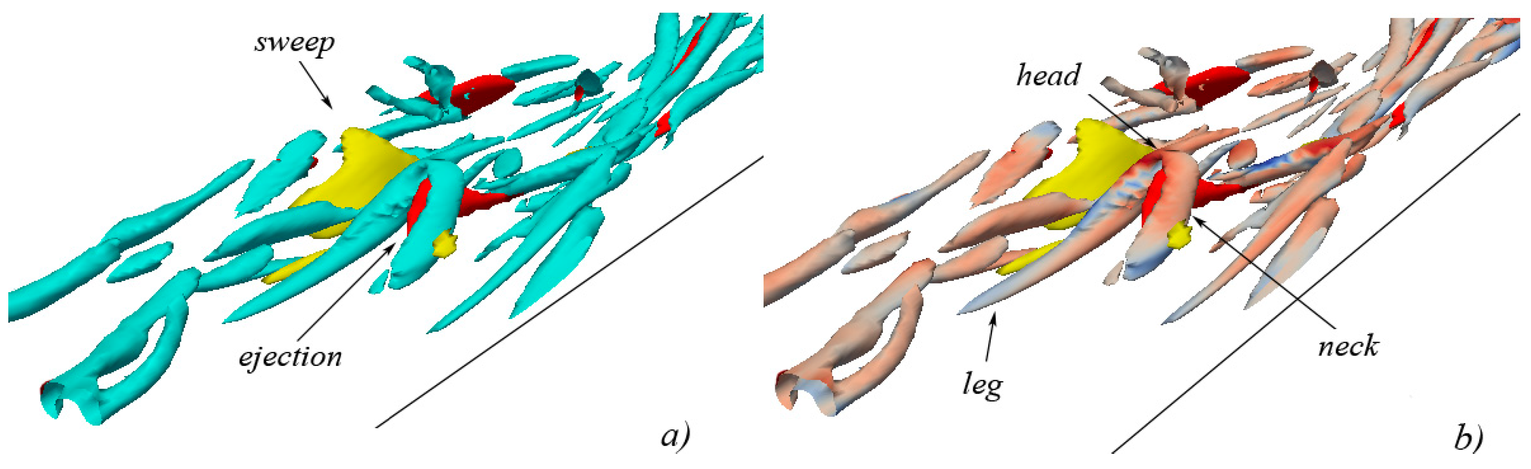
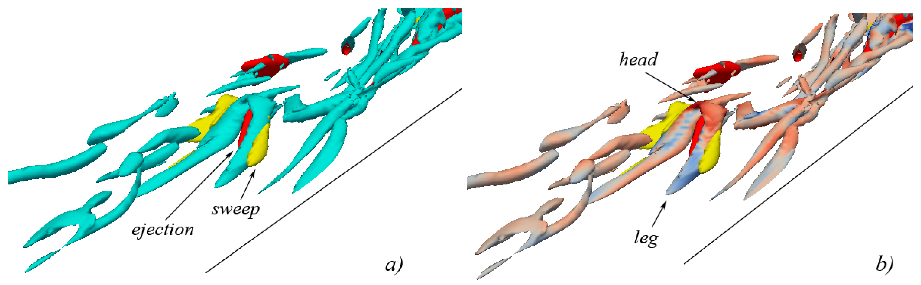
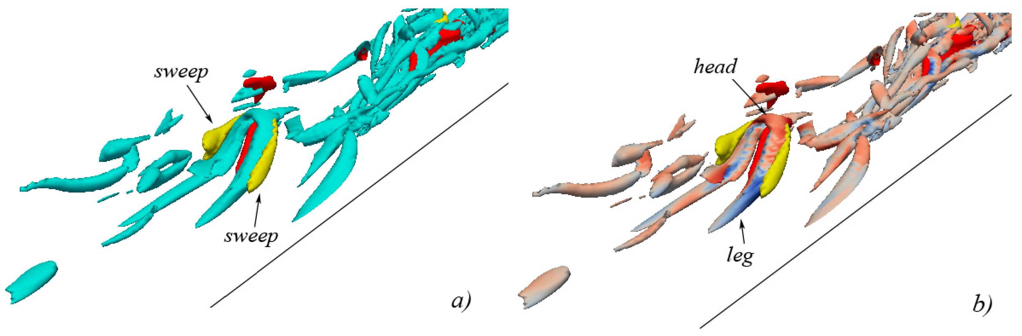
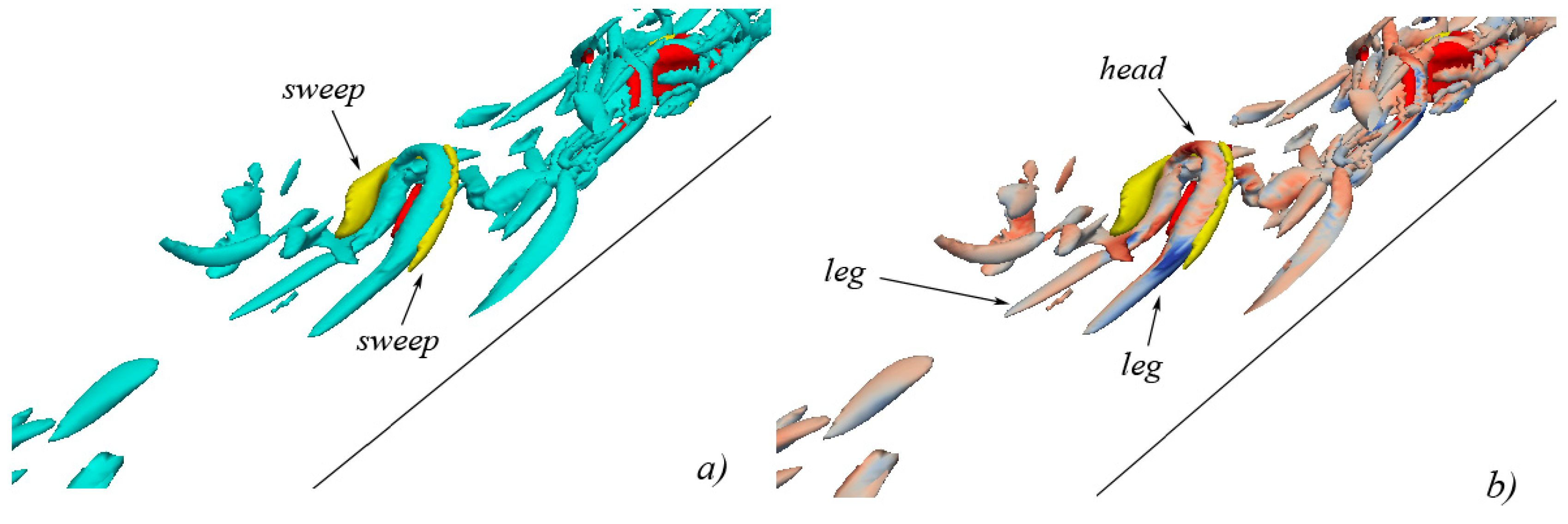
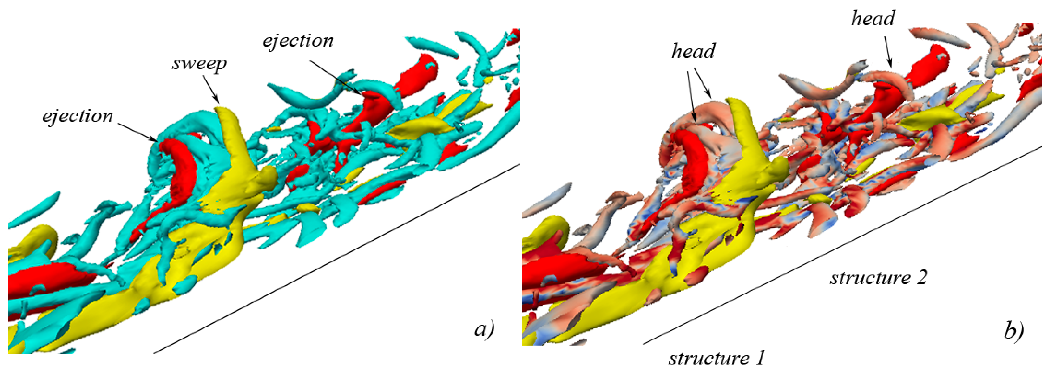
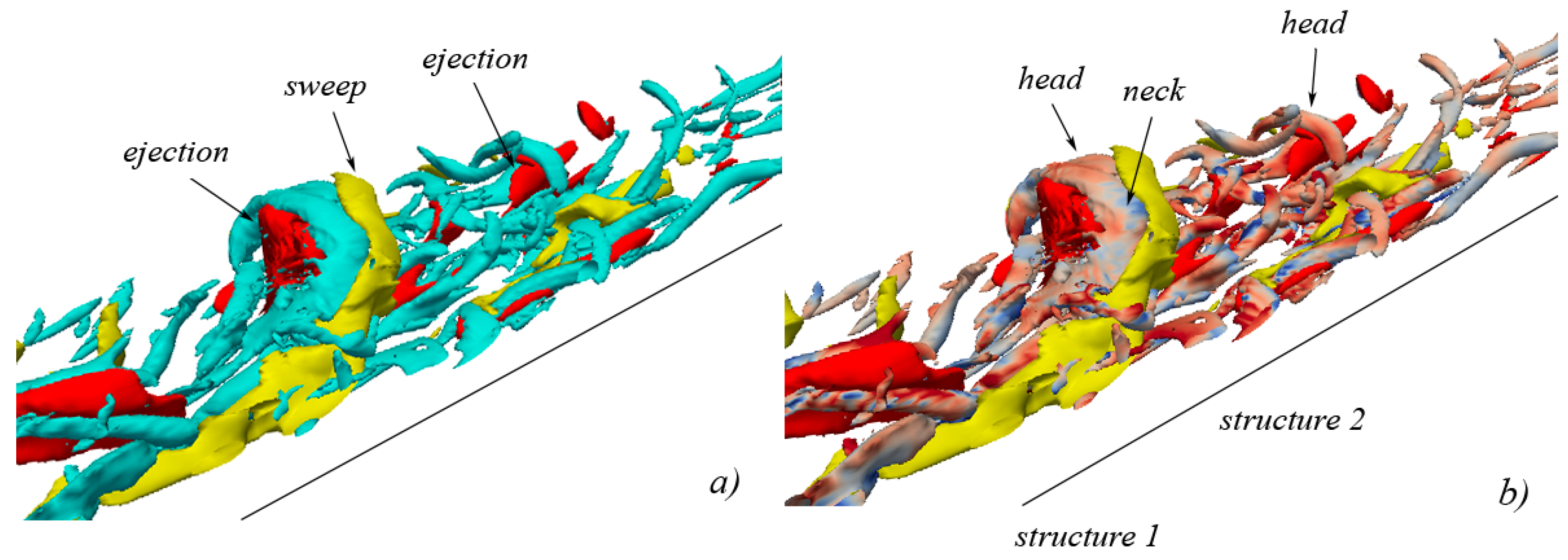
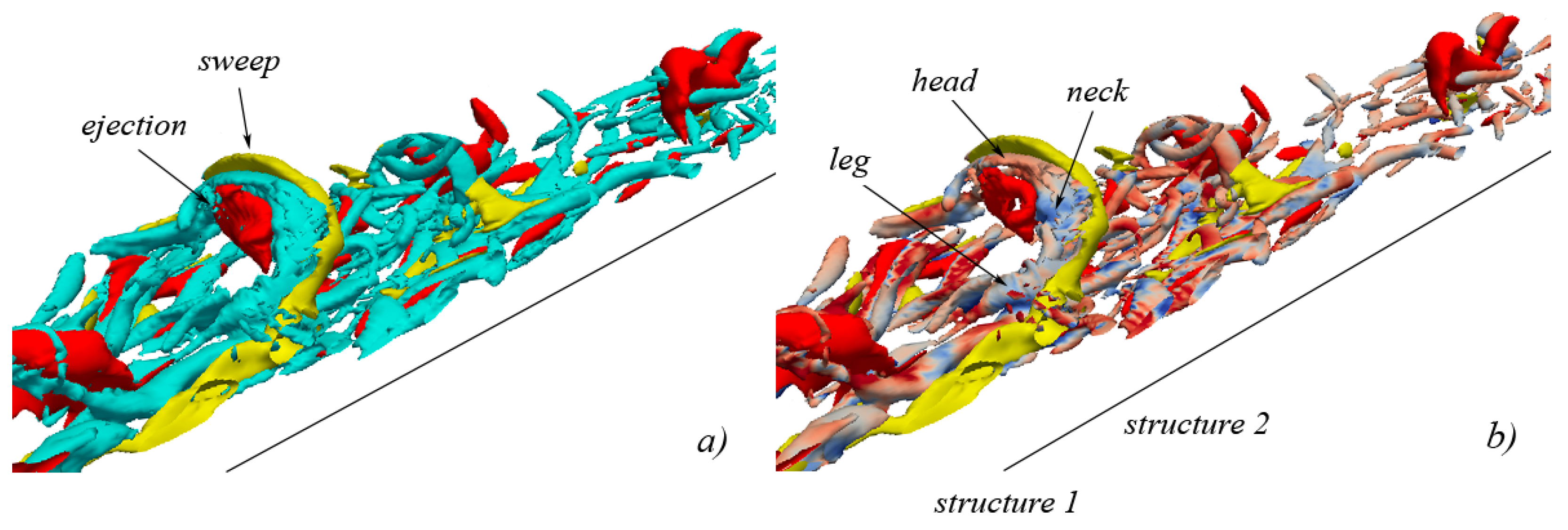
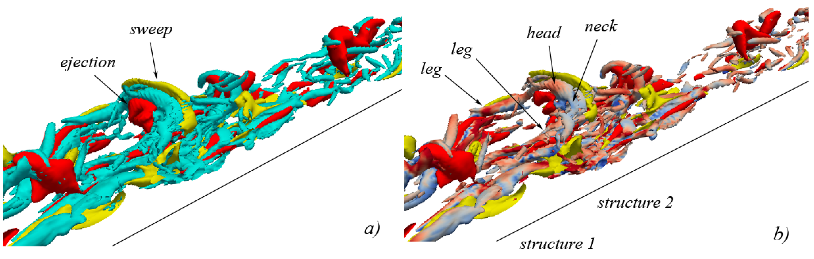
the development of ejections distributed on spheric-like isosurfaces behind an initial Ω -shaped vortex filament;
(ii)
the subsequent development of sweeps distributed on elongated isosurfaces adjacent to the external sides of hairpins’ heads and necks.
The present work is organized as follows. Section 2 contains an outline of the numerical technique used for the solution of the Navier-Stokes equations in the plane-channel-flow computing domain, in Section 3 a concise presentation is given of the vortex-detection method used for flow-structure extraction, and in Section 4, the numerical simulations are described. In Section 5, the results are presented and compared with data obtained by other authors, mainly in terms of turbulence statistics, while in Section 6, the results of the simulations are presented in terms of vortical structures and quadrant events. Concluding remarks are given at the end.

2. Numerical Techniques

The three-dimensional time-dependent Navier-Stokes equations for incompressible fluids are considered in non-dimensional, conservative form (Einstein summation convention applies to repeated indices, i, j = 1, 2, 3):
u i t + x j ( u i u j ) = p x i + 1 R e τ 2 u i x j x j
u i x i = 0
Variables and operators are nondimensionalized by the channel half-height ( h ) for lengths, the wall-shear velocity ( u τ ) for velocities, the group ( ρ u τ 2 ) for pressure, and ( h / u τ ) for time, being R e τ = u τ h / ν the friction-velocity Reynolds number ( ρ is fluid density, ν is fluid kinematic viscosity. Note that, for simplicity, the symbols of both dependent and independent variables have not been altered in switching from the dimensional to the dimensionless formalism). The computing domain (Figure 1) is considered homogeneous along the x (streamwise) and z (spanwise) directions, so that Equations (1) and (2) are Fourier-transformed accordingly:
u ^ t + i k x ( u 2 ^ ) + ( u v ^ ) y + i k z ( u w ^ ) + i k x p ^ = 1 R e τ ( 2 u ^ y 2 k 2 u ^ )
v ^ t + i k x ( v u ^ ) + ( v 2 ^ ) y + i k z ( v w ^ ) + p ^ y = 1 R e τ ( 2 v ^ y 2 k 2 v ^ )
w ^ t + i k x ( w u ^ ) + ( w v ^ ) y + i k z ( w 2 ^ ) + i k z p ^ = 1 R e τ ( 2 w ^ y 2 k 2 w ^ )
i k x u ^ + v ^ y + i k z w ^ = 0
where the superscript (^) indicates variables in Fourier space, and k 2 = k x 2 + k z 2 . The nonlinear terms in the momentum Equations (3a–c) are evaluated pseudospectrally by anti-transforming the velocities in physical space to perform the products (FFTs are used). Here, in order to avoid errors in transforming the results back to Fourier space, the discrete Fourier transforms are applied on “3n/2” points along each homogeneous direction.
Due to the presence of the steepest variable-gradients near the walls, and in order to obtain a suitable spatial resolution in the calculations, a grid-stretching law of hyperbolic tangent type is used for the grid points along y (the direction orthogonal to the walls):
y s t r = P P y + ( 1 P P ) ( 1 t a n h [ Q Q ( 1 y ) ] t a n h [ Q Q ] )
where y indicates the uniform grid and PP, QQ are two parameters characterising the distribution. The partial derivatives along y are calculated according to grid-point distribution Equation (5) using second-order centered finite-difference expressions. For time advancement, the third-order Runge-Kutta procedure originally introduced by Le and Moin [31] is implemented. For each Fourier mode one has:
u ^ i ( l ) u ^ i ( l 1 ) Δ t = α l D ( u ^ i ( l 2 ) ) + β l D ( u ^ i ( l 1 ) ) γ l C ( u ^ i ( l 1 ) ) ζ l C ( u ^ i ( l 2 ) ) ( α l + β l ) p ^ ( l ) x i
where l = 1,2,3 denote the Runge-Kutta sub-steps, and where:
C ( u ^ i ) = x j ( u i u j ) = i k x ( u i u ^ ) + ( u i v ^ ) y + i k z ( u i w ^ )
D ( u ^ i ) = 1 R e τ 2 u i x j x j = 1 R e τ ( 2 u ^ i y 2 k 2 u ^ i )
are the advective- and diffusive terms, respectively. Both terms are treated explicitly and, in Equation (6), α l , β l , γ l , ζ l assume constant values, so that the time advancement results are third-order accurate in the convective part, and second-order accurate in the diffusive:
α 1 = 4 15 , α 2 = 1 15 , α 3 = 1 6 ; β 1 = 4 15 , β 2 = 1 15 , β 3 = 1 6 ; γ 1 = 8 15 , γ 2 = 5 12 , γ 3 = 3 4
ζ 1 = 0 , ζ 2 = 17 60 , ζ 3 = 5 12 ;   l = 1 3 ( α l + β l ) = l = 1 3 ( γ l + ζ l ) = 1
Time marching is coupled with the fractional-step method. In Equation (6), the velocity and pressure fields are decoupled, so that two distinct expressions are generated. At each Runge-Kutta sub-step ( l ) and for each Fourier mode (^), an intermediate velocity field is introduced (superscript *):
u ^ i * ( l ) u ^ i ( l 1 ) Δ t = α l D ( u ^ i ( l 2 ) ) + β l D ( u ^ i ( l 1 ) ) γ l C ( u ^ i ( l 1 ) ) ζ l C ( u ^ i ( l 2 ) )
u ^ i ( l ) u ^ i * ( l ) Δ t = ( α l + β l ) p ^ ( l ) x i
where, by applying the divergence operator to Equation (11) (and so enforcing mass conservation) one obtains a Poisson equation for the pressure, to be solved at each sub-step (l):
2 p ^ ( l ) = 1 Δ t ( α l + β l ) ( u ^ * ( l ) x + v ^ * ( l ) y + w ^ * ( l ) z )
The final values of the velocity are obtained from Equation (11). No-slip boundary conditions at the walls, and cyclic conditions in the streamwise and spanwise directions, have been applied to the velocity (for further details on the numerical algorithm one can refer to Passoni et al. [32,33,34]).

3. Flow-Structure Extraction

Among the different techniques used for the extraction of the coherent structures of turbulence (see Wallace [35], Alfonsi [36], Alfonsi and Primavera [37,38], among others), the swirling-strength criterion as devised by Zhou et al. [30] has been used. The latter is concisely summarized here.
By considering the system of the governing equations, an arbitrary point O can be chosen in the field, and a Taylor-series expansion of each velocity component can be performed in terms of space coordinates with the origin at O, so that the first-order pointwise linear approximation at that point becomes:
u i = A i + A i j x j
( A i j = u i / x j is the velocity-gradient tensor). If O is located at a critical point, the zero-order terms in Equation (13) are zero. From the characteristic equation of A i j one has:
λ 3 + P λ 2 + Q λ + R = 0
where:
P = t r ( A i j ) ;   Q = 1 2 { [ t r ( A i j ) ] 2 t r ( A i j 2 ) } ;   R = det ( A i j )
are the scalar invariants of the velocity-gradient tensor (tr is trace, det is determinant). In the case of incompressible flow, P = 0 , and:
λ 3 + Q λ + R = 0
Q = 1 2 t r ( A i j 2 )
where the discriminant of the characteristic equation of A i j becomes:
D s c = R 2 4 + Q 3 27
When D s c > 0 , the velocity-gradient tensor has one real eigenvalue ( λ 1 = λ r ), and a pair of complex-conjugate eigenvalues ( λ 2 , λ 3 = λ c r ± i λ c i ). Zhou et al. [30] adopted the criterion of identifying vortices by visualizing isosurfaces of prescribed values of the imaginary part of the complex-eigenvalue pair of the velocity-gradient tensor. The swirling strength ( λ c i ) represents a measure of the local swirling rate inside a vortical structure, so that isosurfaces of the imaginary part of the complex eigenvalue pair of the velocity-gradient tensor can be used to visualize vortices (the strength of stretching or compression is given by λ r ). The method is frame independent. It automatically eliminates regions having no local spiralling motion (due to the fact that the eigenvalues are complex only in regions of local circular or spiralling streamlines), and has proven to give rather satisfactory results in several different cases (see [39], among others). As concerns the choice of the threshold value of the swirling strength chosen for structure representation ( λ c i | t h ), one can refer to Alfonsi and Primavera [40].

4. Numerical Simulations

Direct numerical simulations have been executed in the plane-channel domain (Figure 1) with dimensions, grid points, resolutions and Reynolds numbers as reported in Table 2.
As concerns the calculation of the Kolmogorov microscales, they have been evaluated by estimating the average rate of dissipation of turbulent kinetic energy per unit mass ( ε ).
This method was first introduced by Bakewell and Lumley [41], where in the case of the plane channel, one has:
ε 2 L x L z τ w u b 2 ρ h L x L z = u τ 2 u b
The calculations have been executed on a specially-assembled hybrid multicore/manycore computing architecture. The system includes:
(i)
2 Intel Xeon 5660 exa-core CPU processors (12 cores) at 2.8 GHz, with 48 GB GDDR3 RAM;
(ii)
3 Nvidia C-1060 (Tesla) 240-core GPU boards (720 computing cores) at 1.3 GHz, each with 4 GB GDDR3 RAM at 102 GB/s (12 GB available);
(iii)
1 Nvidia GTS-450 (GeForce) 192-core GPU board at 1804 MHz, with 1 GB GDDR5 RAM at 57.7 GB/s (mainly used for visualization);
(iv)
storage system including 5 Hard Drives at 7200 rpm, for a total supply of 5 TB.
Each GPU Nvidia C-1060 board handles a multiprocessor unit, the latter organized in 30 processors. Each processor includes eight floating-point units, 16 kB shared memory, and 4 GB of GDDR3 memory at 102 GB/s bandwidth. The process of implementation of the numerical algorithm (Section 2) on the above computing architecture is described in detail in Alfonsi et al. [42]. The possibility of running the computational code on different partitions of the hybrid computing machine has enabled the execution of the numerical simulations in remarkably limited runtimes (Table 3). According to a procedural viewpoint, the initial transient of the flow in the channel has been first simulated, the turbulent statistically-steady state has been reached, and thereafter (for each value of the Reynolds numbers tested) 500,000 time steps of the statistical steady state have been gathered, with temporal resolution Δ t = 1 × 10 4 h / u τ . The flow fields have been saved every given Δ t interval, finally giving a 500· Δ t + database for each of the Reynolds numbers tested. The adequacy of length and span of the computing domain has been tested by verifying that the velocity fluctuations at streamwise and spanwise separations on half the domain dimensions were uncorrelated. The adequacy of the grid resolution has been also tested, through the analysis of the one-dimensional energy spectra. It has been verified that the energy densities associated to the high wavenumbers are up to nine orders of magnitude lower than those corresponding to the low wavenumbers (for more details on these issues one can refer to Ciliberti [43]).

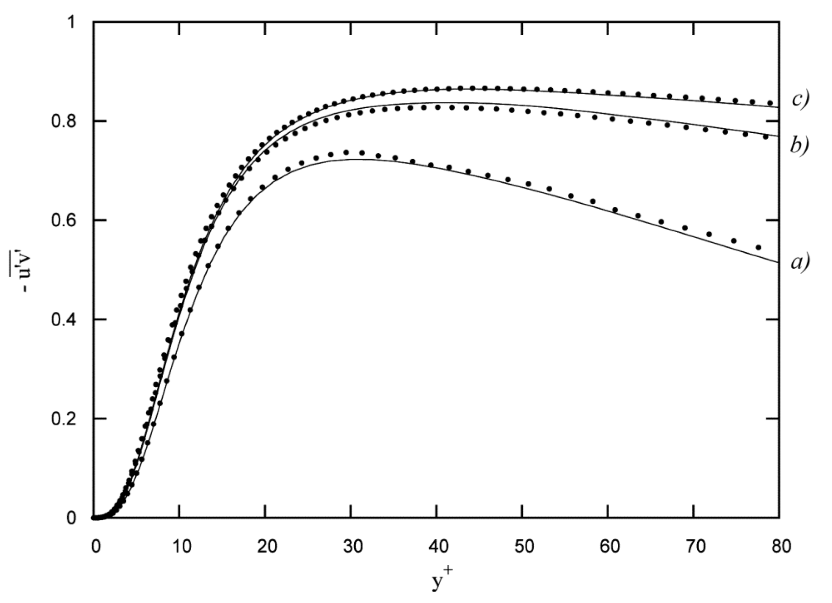
5. Turbulence Statistics
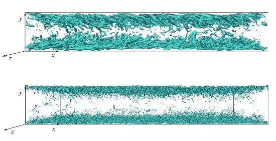
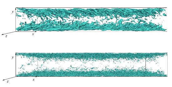
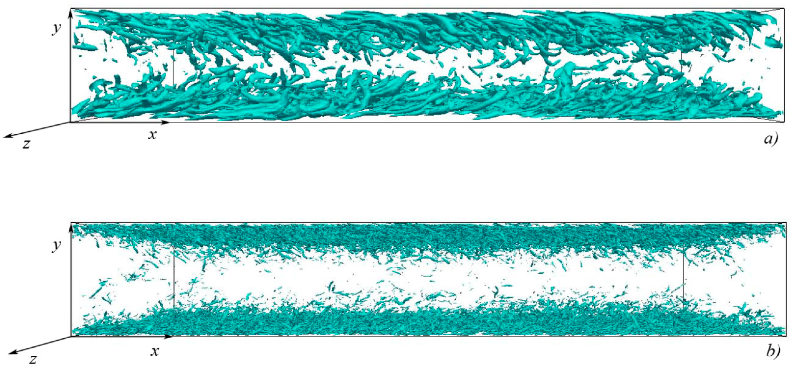
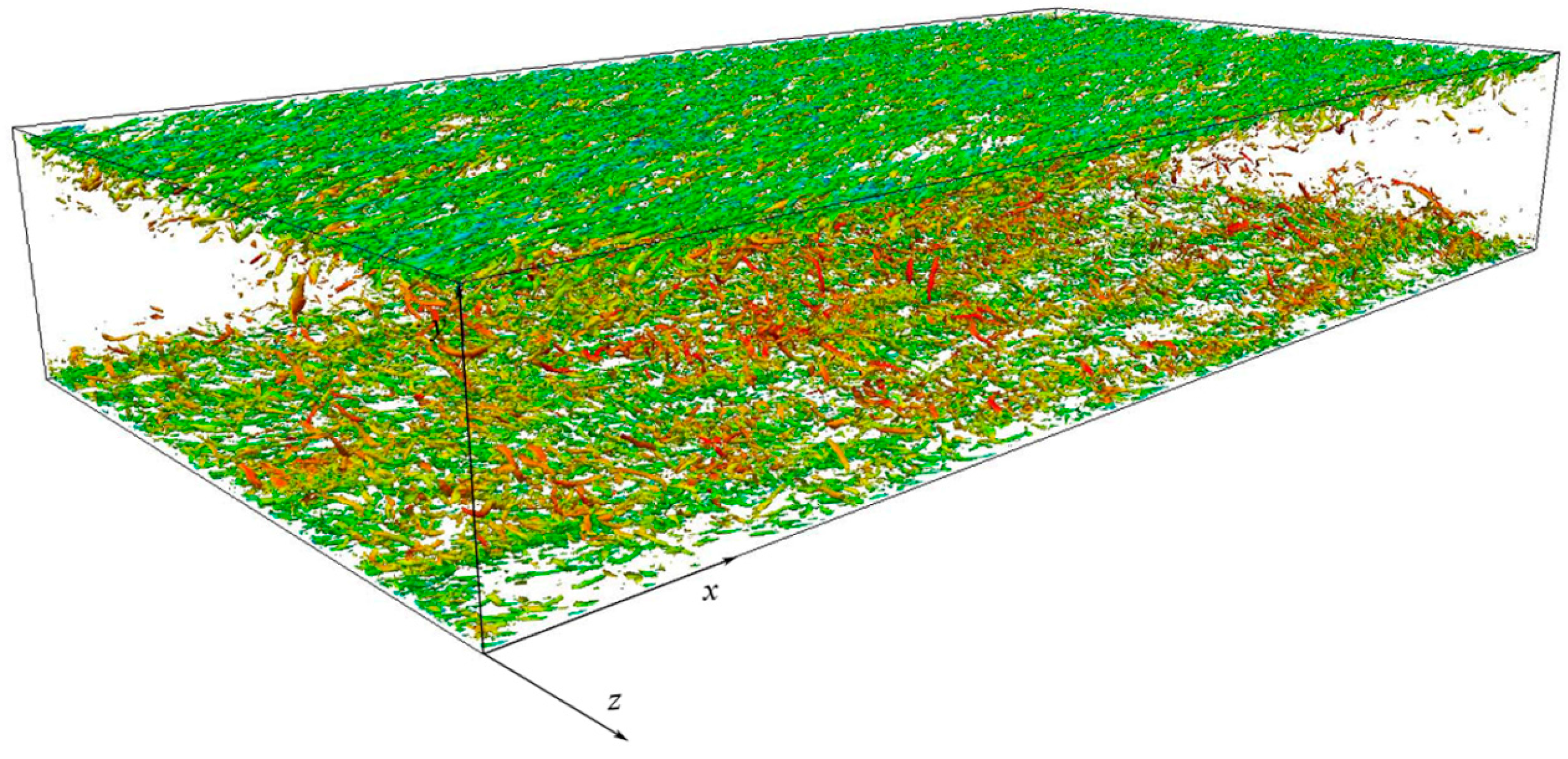
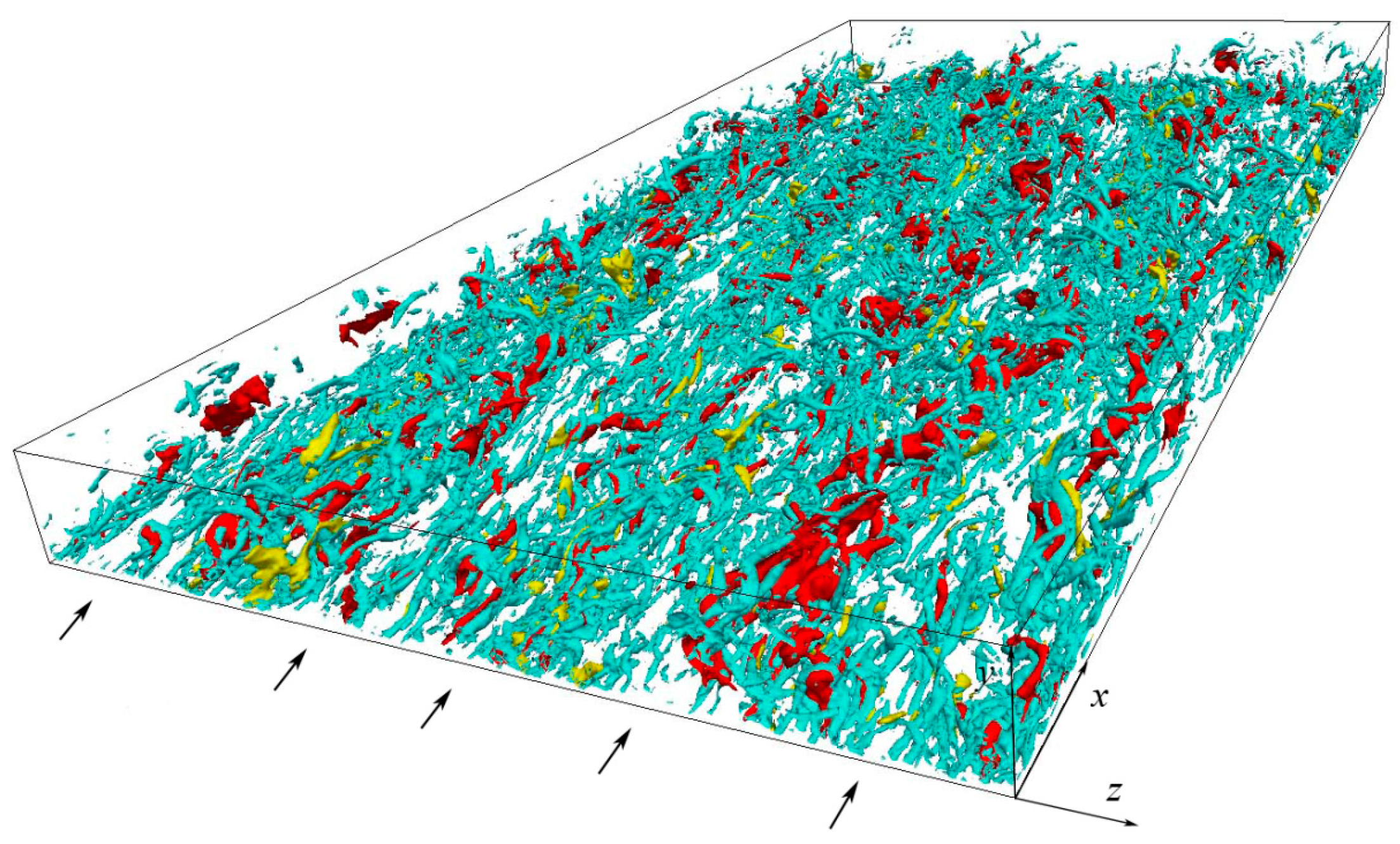
In Table 4 and Figure 2, Figure 3, Figure 4, Figure 5 and Figure 6, results are presented in terms of turbulence statistics. Figure 2 reports the values of the Reynolds shear stress ( u v ¯ ) in wall coordinates, in a comparison with the data.
Figure 3 reports the rms values of the velocity fluctuations ( u r m s , v r m s , w r m s ) in a comparison with those of Moser et al. [6]. In a similar manner, Figure 4 reports the skewness factors of the velocity fluctuations ( S u , S v , S w ), and Figure 5 the flatness factors ( F u , F v , F w ). In Figure 6, the values of the production terms ( P K ), the transport terms ( T K ), the diffusion terms ( D K ), and the dissipation terms ( ε K ) of the turbulent-kinetic-energy transport equation ( K = u i u i ¯ / 2 ), as calculated in the present work, are reported, again in a comparison with Moser et al. [6].
As concerns mean-flow quantities, in Table 4 the values of a number of quantities [ u τ , u b , u c , ( u b / u τ ), ( u c / u τ ), ( u c / u b ), C f b ] as calculated in the present work are reported in a comparison with the experimental data of Dean [44]. As for mean-velocity distribution, the linear distribution ( u + = y + ) is satisfactorily followed in the viscous sublayer ( y + < 5 ), while at larger distances from the wall ( y + > 30 ), the logarithmic distribution ( u + = 1 κ l n y + + C ) is also satisfactorily followed, with κ = 0.4 and C = 5.5 (not shown).
As concerns fluctuating velocity components (Table 4), the peak values of the Reynolds shear stress ( u v ¯ | p e a k ), those of the rms-fluctuating streamwise velocities ( u r m s | p e a k ), and the fluctuating streamwise velocities skewness factors ( S u | p e a k ) [and their positions ( y + | p e a k u v ¯ , y + | p e a k u r m s , y + | p e a k S u )], exhibit a good agreement with the values of Moser et al. [6]. Moreover, it has been found that the peak values of the rms-fluctuating streamwise velocities and their positions satisfactorily follow the expressions devised by Mochizuki and Nieuwstadt [45] as a function of R e τ , as deduced from the analysis of a large number of experimental works (see also Alfonsi [46]):
u r m s | p e a k = 0.0000024 R e τ + 2.70
y + | p e a k u r m s = 0.00020 R e τ + 14.6
The values of the skewness factors of the streamwise fluctuations ( S u , Figure 4) are rather close to zero at the position of rms-fluctuating-streamwise-velocities peak values ( y + | p e a k u r m s ) and, except for these latter positions, are significantly different from the Gaussian values. The values of the flatness factors of the wall-normal fluctuations ( F v , Figure 5) also significantly differ from the Gaussian ones, and assume remarkably-high values approaching the walls, so unveiling the highly-intermittent character of the normal-velocity fluctuations near the walls. In particular (Table 4), approaching the walls, the flatness factor F v assumes values that result in an excellent agreement with the data of Moser et al. [6] (see also at Xu et al. [47] and Alfonsi [48]).
By looking at the budgets of the mean turbulent kinetic-energy ( K , Figure 6), it can be noted that, at y + > 30 , the homogeneous character of the flow is reasonably confirmed, while, moving toward the wall, the turbulent-transport rate becomes relevant. The turbulent-transport term is a consuming term approaching the wall, and a producing term near the wall. Close to the wall, the dissipation rate balances the viscous-diffusion and pressure-diffusion rates, and, at the wall, the dissipation rate is nonzero, while being almost equal to the viscous-diffusion rate.
Overall, the comparison of the results of present work with data obtained by other authors, both numerically and experimentally, is rather satisfactory.

6. Flow Structures

After the application of the λ c i vortex-detection technique (Section 3), the flow field in the channel appears to be highly populated by turbulent structures adjacent to both the upper and the lower wall of the computing domain, with a wide range of inclination angles. The majority of them has no definite shape. Side views of the phenomenon (at R e τ = 200 and R e τ = 600 ) are given in Figure 7 at a generic instant. It can be noticed how the turbulent structures are noticeably smaller in size and more numerous in the case of R e τ = 600 with respect to R e τ = 200 , as expected. In particular, Figure 7 shows that several structures also exist outside the buffer layer, protruding toward the center of the channel. Figure 8 shows a general view of vortical structures at R e τ = 600 on both walls of the computing domain. Here, the external surfaces of the structures are colored with the values of the local streamwise velocity (reddish indicates high values, greenish indicates low values). It can be noted, as expected, how the streamwise velocities increase towards the center of the computing domain, with respect to the more peripheral zones. Figure 9 shows a general view of vortical structures in conjunction with isosurfaces of Q 2 and Q 4 quadrant events (ejection and sweeps) at R e τ = 400 , on the lower wall of the computing domain, at a generic instant. It can be noticed how flow structures and quadrant events are more densely located in streamwise-elongated zones of the domain, the latter being separated from the adjacent by low-speed streaks (arrows, see also Kline et al. [49]).
Through Figure 10, Figure 11, Figure 12 and Figure 13, the process of evolution in time is shown with a single hairpin-like vortical structure. At t + = 450 (Figure 10), the onset is represented by the process of formation of a single, isolated, two-leg, symmetric and stable hairpin. It can be noted how an ejecting surface is pushing the perspective hairpin upwards (actually a Ω-shaped vortex filament) while, mainly on its left side (the flow goes from left to right), a sweeping surface starts to develop. Moreover, Figure 10b shows that the head of the structure is subjected to stretching, while the neck and legs are subjected to compression.
The process continues through instants t + = 451 and t + = 452 (Figure 11 and Figure 12) during which the ejecting surface keeps pushing the head of the structure upwards, and the sweeping surface, adjacent to the right side of the structure, further grows, so that both the right and the left portions of the structure neck become adjacent, externally to the sweeping isosurface, and internally to the ejecting isosurface. The head of the structure (Figure 11b and Figure 12b) continues to be stretched under the action of the ejecting surface, while neck and legs are subjected to compression, due to the action of the sweeping surfaces.
At instant t + = 453 (Figure 13) the ejecting surface starts to extinguish, while the sweeping surface now exerts its characteristic stabilizing action onto the entire external structure of the now fully-formed hairpin vortex (head, neck and legs). From Figure 13b it can be also noted that the head of the vortical structure is subjected to a less intense stretching, due to the gradual process of extinction of the previously upward-pushing underlying ejecting isosurface, while the legs of the structure are subjected to compression when subjected to the action of the overlying sweeping surfaces.
Figure 14, Figure 15, Figure 16 and Figure 17 show the evolution in time of a more complex aggregate of vortical structures in a different portion of the computing domain.
At t + = 220 (Figure 14) two main primary Ω-shaped vortex filaments are visible at the center of the field (arrows). Right below the head of each filament, the internal space of the structure is occupied by an ejecting isosurface, again showing that, in this initial phase, ejections represent the main mechanism according to which the heads of the structures are raised upwards. Correspondingly (Figure 14b), the process of progressive stretching of the vortex head (actually still a double head) also starts.
In Figure 15, the flow field at t + = 221 is shown. The heads of both structures 1 and 2 continue to raise (being subjected to stretching, Figure 15b) due to the upward-pushing action of the ejections. The sweeping surface mainly maintains its position adjacent to the right side of hairpin 1, causing the compression of the contiguous vortical-structure neck (Figure 15b). Note again that the ejecting isosurface below hairpin 1 is almost equally developed in the streamwise, spanwise and normal-to-the-wall directions (a spheric-like surface), so guaranteeing that the pushing action of the ejecting surface against the internal part of the vortical structure is exerted almost uniformly. It can be also noticed that the presence of sweeping isosurfaces adjacent to hairpin 2 is not so evident as in the case of hairpin 1, and this is the reason why vortex 2 will be destroyed much sooner with respect to vortex 1 (not shown). At t + = 222 (Figure 16), the vortical structures continue their development. The heads of hairpins 1 and 2 continue to raise under the residual influence of the ejection events (the underlying ejecting isosurfaces are now reduced) while a well-defined sweeping isosurface assumes its definite position, adjacent to the external side of head, neck and legs of hairpin 1. The action of compression (Figure 16b) exerted by the sweeping vortex-overlying surface, in particular onto the neck of hairpin 1, becomes more intense. At t + = 223 (Figure 17), the process of evolution of the vortical structures continues in a similar manner, with respect to the previous instants. The action of the ejection events is decreasing, while the sweeping isosurface acts towards the maintenance of the stability of hairpin 1. Also, in this case, the result is hairpin 1 becoming a two-leg, symmetric, and stable vortical structure.

7. Concluding Remarks

The Direct Numerical Simulation (DNS) of the turbulent flow of incompressible fluid in a plane channel has been executed at three values of the friction-velocity Reynolds number, using a hybrid CPU/GPU computing architecture, and an analysis has been performed of the characteristics of the vortical structures in the wall region of the turbulent channel flow. Turbulent flow structures have been extracted from the simulated flow fields using the λ c i or swirling strength criterion, as devised by Zhou et al. [24].
The joint analysis of hairpin vortices and ejection/sweep quadrant events has led to the following conclusions:
(i)
the physical condition for the development and subsequent morphological evolution of a stable hairpin-like vortical structure is the occurrence of ejections distributed onto an isosurface almost equally developed along the streamwise, spanwise and normal-to-the-wall directions (a spheric-like isosurface) behind an initially connected Ω-shaped vortex filament, lying near the wall. These ejections actually constitute the physical mechanism according to which the head of the hairpin is raised upward;
(ii)
the physical condition for the development of a complete and persistent hairpin is the subsequent occurrence of sweeps, as distributed on elongated isosurfaces adjacent to the external sides of the neck and legs of the hairpin.
The sweeps actually constitute the physical mechanism according to which:
(ii/a)
the legs of the hairpin are stably kept near the wall;
(ii/b)
the right portion (leg and neck) of the hairpin is characterized by local clockwise particle rotation, the left portion (leg and neck) by counter clockwise local particle rotation.

Author Contributions

All the authors contributed equally to this paper.

Conflicts of Interest

The authors declare no conflict of interest.

Nomenclature

Roman symbols (upper case)
A i j = u i / x j velocity-gradient tensor
C f b = 2 τ w / ρ u b 2 bulk-velocity friction coefficient
D s c discriminant of characteristic equation
D K 
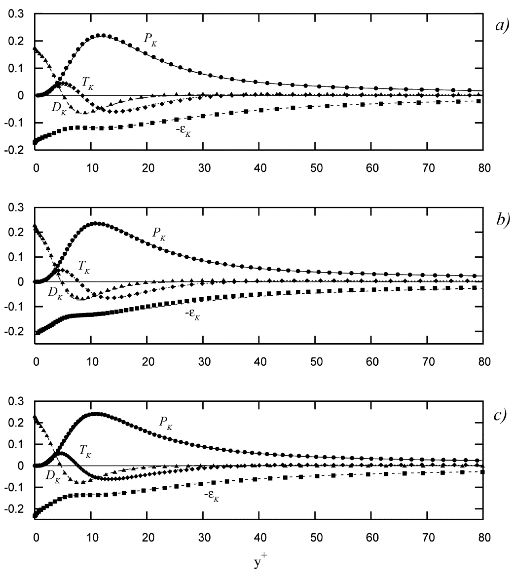
viscous-diffusion term of turbulent kinetic-energy transport equation
F u , F v , F w 
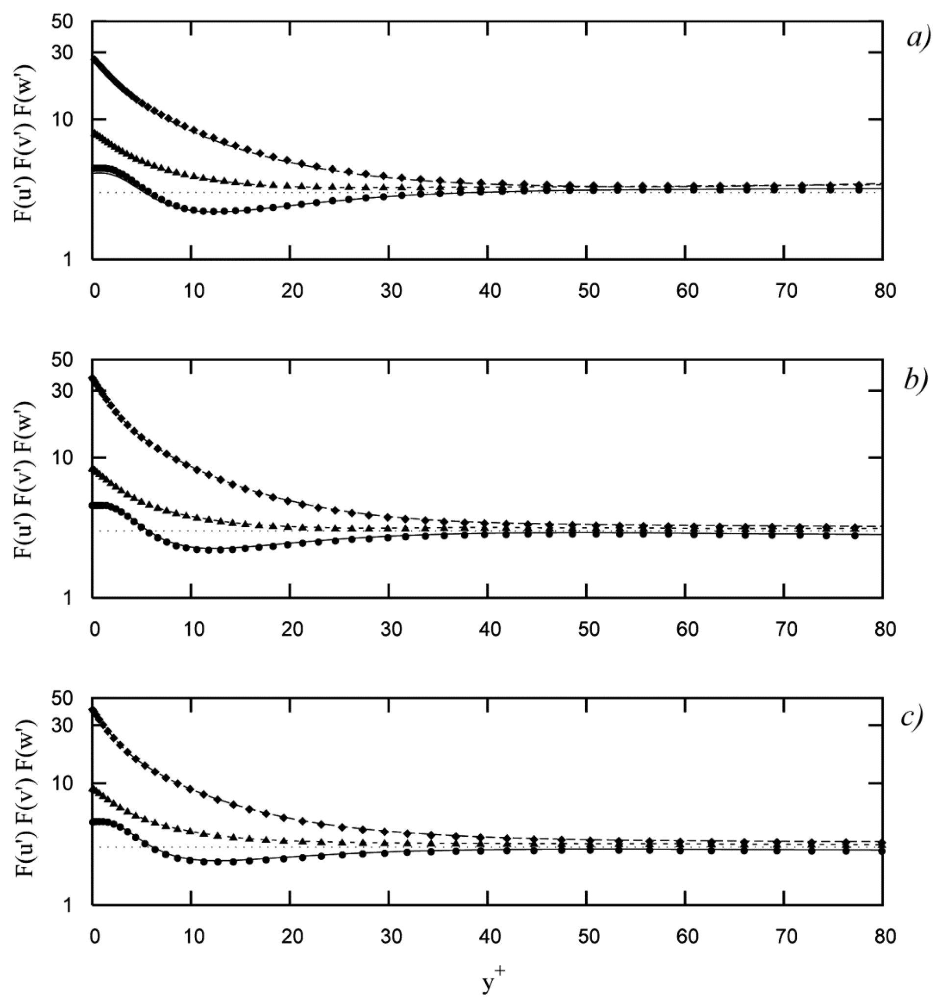
flatness factors of velocity fluctuations
F v | p e a k peak value of F v
K = u i u i ¯ / 2 mean turbulent kinetic energy
L x , L y , L z 
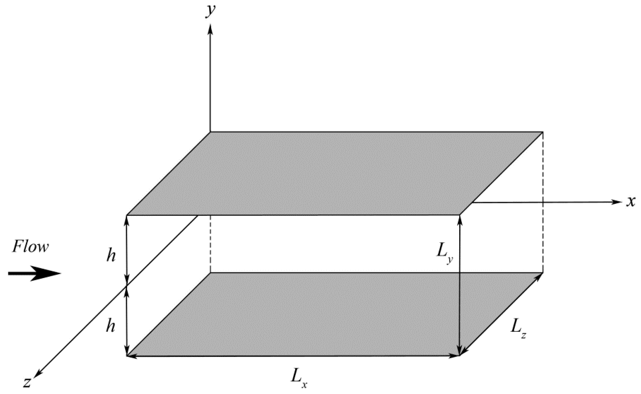
domain dimensions along x,y,z (h units)
L x + , L y + , L z + domain dimensions along x,y,z (wall units)
N x , N y , N z number of grid points along x,y,z
N t o t total number of grid points
P K production term of turbulent kinetic-energy transport equation
P , Q , R scalar invariants of velocity-gradient tensor
P P , Q Q parameters in the grid-stretching law
Q 2 second-quadrant event (ejection)
Q 4 fourth-quadrant event (sweep)
R e τ = u τ h / ν friction-velocity Reynolds number
S u , S v , S w 
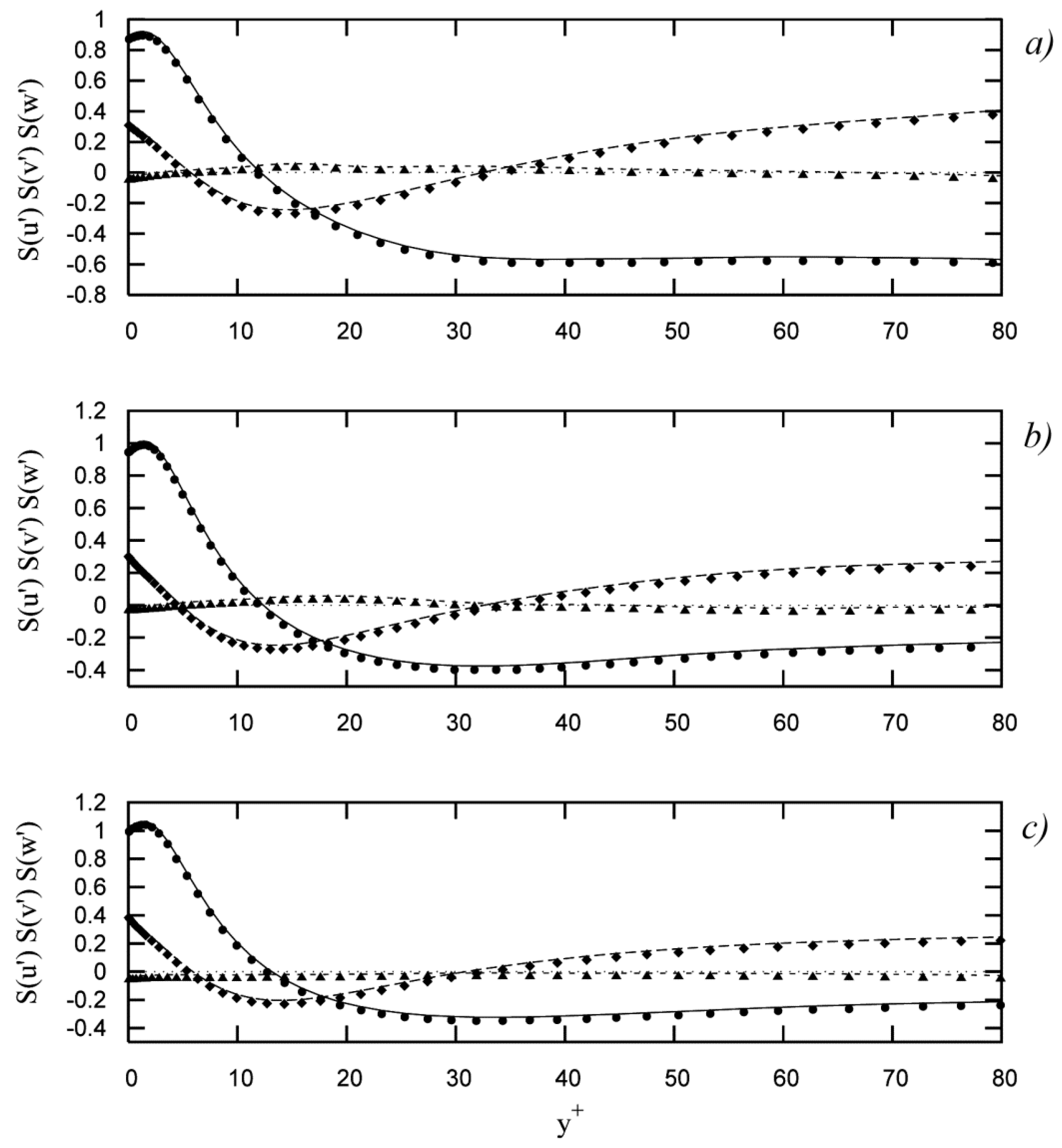
skewness factors of velocity fluctuations
S u | p e a k peak value of S u
T K transport term of turbulent kinetic-energy transport equation
Roman symbols (lower case)
h channel half-height
k wavenumber
p pressure
t time coordinate
t + time coordinate (wall units)
t D B t o t total database calculated time
t D B + | s a v e d actually saved database calculated time (wall units)
u i ( u , v , w ) velocity components along x,y,z
u i ( u , v , w ) fluctuating-velocity components along x,y,z
u r m s , v r m s , w r m s rms velocity fluctuations
u r m s | p e a k peak value of u r m s
u v ¯ Reynolds shear stress
u v ¯ | p e a k peak value of u v ¯
u b bulk velocity
u c centerline velocity
u τ friction velocity
x i ( x , y , z ) Cartesian coordinates
x i + ( x + , y + , z + ) Cartesian coordinates (wall units)
y + | p e a k u r m s y-position of u r m s | p e a k (wall units)
y + | p e a k u v ¯ y-position of u v ¯ | p e a k (wall units)
y + | p e a k S u y-position of S u | p e a k (wall units)
y + | p e a k F v y-position of F v | p e a k (wall units)
Greek symbols (upper case)
Δ t + time resolution of calculations (wall units)
Δ x + , Δ z + space resolution of calculations along x,z (wall units)
Δ y w a l l + space resolution of calculations along y at channel wall (wall units)
Δ y c e n t e r + space resolution of calculations along y at channel center (wall units)
Greek symbols (lower case)
ε average rate of dissipation of turbulent kinetic energy per unit mass
ε K dissipation term of mean turbulent kinetic-energy transport equation
η + Kolmogorov space microscale (wall units)
λ eigenvalue
λ r real eigenvalue
λ c r real part of complex eigenvalue
λ c i imaginary part of complex eigenvalue
( λ c i ) t h threshold value of swirling strength
ν fluid kinematic viscosity
ρ fluid density
τ w mean shear stress at wall
τ η + Kolmogorov time microscale (wall units)
Acronyms
CPUCentral Processing Unit
DNSDirect Numerical Simulation (of turbulence)
GPUGraphic Processing Unit

References

  1. Kim, J.; Moin, P.; Moser, R. Turbulence statistics in fully developed channel flow at low Reynolds number. J. Fluid Mech. 1987, 177, 133–166. [Google Scholar] [CrossRef]
  2. Lyons, S.L.; Hanratty, T.J.; McLaughlin, J.B. Large-scale computer simulation of fully developed turbulent channel flow with heath transfer. Int. J. Num. Meth. Fluids 1991, 13, 999–1028. [Google Scholar] [CrossRef]
  3. Antonia, R.A.; Teitel, M.; Kim, J.; Browne, L.W.B. Low-Reynolds-number effects in a fully developed turbulent channel flow. J. Fluid Mech. 1992, 236, 579–605. [Google Scholar] [CrossRef]
  4. Kasagi, N.; Tomita, Y.; Kuroda, A. Direct numerical simulation of passive scalar field in a turbulent channel flow. ASME J. Heat Transf. 1992, 114, 598–606. [Google Scholar] [CrossRef]
  5. Rutledge, J.; Sleicher, C.A. Direct simulation of turbulent flow and heat transfer in a channel. Part I: Smooth walls. Int. J. Num. Meth. Fluids 1993, 16, 1051–1078. [Google Scholar] [CrossRef]
  6. Moser, R.D.; Kim, J.; Mansour, N.N. Direct numerical simulation of turbulent channel flow up to R e τ = 590 . Phys. Fluids 1999, 11, 943–945. [Google Scholar] [CrossRef]
  7. Abe, H.; Kawamura, H.; Matsuo, Y. Direct numerical simulation of a fully developed turbulent channel flow with respect to the Reynolds number dependence. ASME J. Fluids Eng. 2001, 123, 382–393. [Google Scholar] [CrossRef]
  8. Iwamoto, K.; Suzuki, Y.; Kasagi, N. Reynolds number effect on wall turbulence: Toward effective feedback control. Int. J. Heat Fluid Flow 2002, 23, 678–689. [Google Scholar] [CrossRef]
  9. Del Alamo, J.C.; Jiménez, J. Spectra of the very large anisotropic scales in turbulent channels. Phys. Fluids 2003, 15, L41–L44. [Google Scholar] [CrossRef]
  10. Del Alamo, J.C.; Jiménez, J.; Zandonade, P.; Moser, R.D. Scaling of the energy spectra of turbulent channels. J. Fluid Mech. 2004, 500, 135–144. [Google Scholar] [CrossRef]
  11. Tanahashi, M.; Kang, S.J.; Miyamoto, T.; Shiokawa, S.; Miyauchi, T. Scaling law of the fine-scale eddies in turbulent channel flows up to R e τ = 800 . Int. J. Heat Fluid Flow 2004, 25, 331–340. [Google Scholar] [CrossRef]
  12. Iwamoto, K.; Kasagi, N.; Suzuki, Y. Direct numerical simulation of turbulent channel flow at R e τ = 2320 . Available online: http://www.nmri.go.jp/turbulence/PDF/symposium/FY2004/Iwamoto.pdf (accessed on 17 February 2016).
  13. Hoyas, S.; Jiménez, J. Scaling of the velocity fluctuations in turbulent channels up to R e τ = 2003 . Phys. Fluids 2006, 18, 011702. [Google Scholar] [CrossRef]
  14. Hu, Z.W.; Morfey, C.L.; Sandham, N.D. Wall pressure and shear stress spectra from direct simulations of channel flow. AIAA J. 2006, 44, 1541–1549. [Google Scholar] [CrossRef]
  15. Alfonsi, G.; Primavera, L. Direct numerical simulation of turbulent channel flow with mixed spectral-finite difference technique. J. Flow Visual. Image Proc. 2007, 14, 225–243. [Google Scholar]
  16. Lozano-Durán, A.; Flores, O.; Jiménez, J. The three-dimensional structure of momentum transfer in turbulent channels. J. Fluid Mech. 2012, 694, 100–130. [Google Scholar] [CrossRef]
  17. Lozano-Durán, A.; Jiménez, J. Effect of the computational domain on direct simulations of turbulent channels up to R e τ = 4200 . Phys. Fluids 2014, 26, 011702. [Google Scholar] [CrossRef]
  18. Vreman, A.W.; Kuerten, J.G.M. Comparison of direct numerical simulation databases of turbulent channel flow at R e τ = 180 . Phys. Fluids 2014, 26, 015102. [Google Scholar] [CrossRef]
  19. Vreman, A.W.; Kuerten, J.G.M. Statistics of spatial derivatives of velocity and pressure in turbulent channel flow. Phys. Fluids 2014, 26, 085103. [Google Scholar] [CrossRef]
  20. Bernardini, M.; Pirozzoli, S.; Orlandi, P. Velocity statistics in turbulent channel flow up to R e τ = 4000 . J. Fluid Mech. 2014, 742, 171–191. [Google Scholar] [CrossRef]
  21. Lee, M.; Moser, R.D. Direct numerical simulation of turbulent channel flow up to R e τ = 5200 . J. Fluid Mech. 2015, 774, 395–415. [Google Scholar] [CrossRef]
  22. Kim, J.; Moin, P. Application of a fractional-step method to incompressible Navier-Stokes equations. J. Comput. Phys. 1985, 59, 308–323. [Google Scholar] [CrossRef]
  23. Alfonsi, G.; Passoni, G.; Pancaldo, L.; Zampaglione, D. A spectral-finite difference solution of the Navier-Stokes equations in three dimensions. Int. J. Numer. Meth. Fluids 1998, 28, 129–142. [Google Scholar] [CrossRef]
  24. Alfonsi, G. On direct numerical simulation of turbulent flows. Appl. Mech. Rev. 2011, 64, 020802. [Google Scholar] [CrossRef]
  25. Marusic, I.; McKeon, B.J.; Monkewitz, P.A.; Nagib, H.M.; Smits, A.J.; Sreenivasan, K.R. Wall-bounded turbulent flows at high Reynolds numbers: Recent advances and key issues. Phys. Fluids 2010, 22, 065103. [Google Scholar] [CrossRef]
  26. Smits, A.J.; McKeon, B.J.; Marusic, I. High-Reynolds number wall turbulence. Annu. Rev. Fluid Mech. 2011, 43, 353–375. [Google Scholar] [CrossRef]
  27. Kim, J. Progress in pipe and channel flow turbulence, 1961–2011. J. Turbul. 2012, 13. [Google Scholar] [CrossRef]
  28. Jiménez, J. Cascades in wall-bounded turbulence. Annu. Rev. Fluid Mech. 2012, 44, 27–45. [Google Scholar] [CrossRef]
  29. Alfonsi, G.; Primavera, L. Temporal evolution of vortical structures in the wall region of turbulent channel flow. Flow Turbul. Combust. 2009, 83, 61–79. [Google Scholar] [CrossRef]
  30. Zhou, J.; Adrian, R.J.; Balachandar, S.; Kendall, T.M. Mechanisms for generating coherent packets of hairpin vortices in channel flow. J. Fluid Mech. 1999, 387, 353–396. [Google Scholar] [CrossRef]
  31. Le, H.; Moin, P. An improvement of fractional step methods for the incompressible Navier-Stokes equations. J. Comput. Phys. 1991, 92, 369–379. [Google Scholar] [CrossRef]
  32. Passoni, G.; Alfonsi, G.; Tula, G.; Cardu, U. A wavenumber parallel computational code for the numerical integration of the Navier-Stokes equations. Parall. Comput. 1999, 25, 593–611. [Google Scholar] [CrossRef]
  33. Passoni, G.; Cremonesi, P.; Alfonsi, G. Analysis and implementation of a parallelization strategy on a Navier-Stokes solver for shear flow simulations. Parall. Comput. 2001, 27, 1665–1685. [Google Scholar] [CrossRef]
  34. Passoni, G.; Alfonsi, G.; Galbiati, M. Analysis of hybrid algorithms for the Navier-Stokes equations with respect to hydrodynamic stability theory. Int. J. Numer. Meth. Fluids 2002, 38, 1069–1089. [Google Scholar] [CrossRef]
  35. Wallace, J.M. Twenty years of experimental and direct numerical simulation access to the velocity gradient tensor: What have we learned about turbulence? Phys. Fluids 2009, 21, 021301. [Google Scholar] [CrossRef]
  36. Alfonsi, G. Coherent structures of turbulence: Methods of eduction and results. Appl. Mech. Rev. 2006, 59, 307–323. [Google Scholar] [CrossRef]
  37. Alfonsi, G.; Primavera, L. The structure of turbulent boundary layers in the wall region of plane channel flow. Proc. R. Soc. A 2007, 463, 593–612. [Google Scholar] [CrossRef]
  38. Alfonsi, G.; Primavera, L. On identification of vortical structures in turbulent shear flow. J. Flow Visual. Image Proc. 2008, 15, 201–216. [Google Scholar]
  39. Alfonsi, G. Numerical simulations of wave-induced flow fields around large-diameter surface-piercing vertical circular cylinder. Computation 2015, 3, 386–426. [Google Scholar] [CrossRef]
  40. Alfonsi, G.; Primavera, L. Determination of the threshold value of the quantity chosen for vortex representation in turbulent flow. J. Flow Visual. Image Proc. 2009, 16, 41–49. [Google Scholar]
  41. Bakewell, H.P.; Lumley, J.L. Viscous sublayer and adjacent wall region in turbulent pipe flow. Phys. Fluids 1967, 10, 1880–1889. [Google Scholar] [CrossRef]
  42. Alfonsi, G.; Ciliberti, S.A.; Mancini, M.; Primavera, L. GPGPU implementation of mixed spectral-finite difference computational code for the numerical integration of the three-dimensional time-dependent incompressible Navier-Stokes equations. Comput. Fluids 2014, 102, 237–249. [Google Scholar] [CrossRef]
  43. Ciliberti, S.A. Coherent Structures of Turbulence in Wall-Bounded Turbulent Flows. Ph.D. Thesis, Università della Calabria, Rende, Italy, 2011. [Google Scholar]
  44. Dean, R.B. Reynolds number dependence of skin friction and other bulk flow variables in two-dimensional rectangular duct flow. ASME J. Fluids Eng. 1978, 100, 215–223. [Google Scholar] [CrossRef]
  45. Mochizuki, S.; Nieuwstadt, F.T.M. Reynolds-number-dependence of the maximum of the streamwise velocity fluctuations in wall turbulence. Exp. Fluids 1996, 21, 218–226. [Google Scholar] [CrossRef]
  46. Alfonsi, G. Analysis of streamwise velocity fluctuations in turbulent pipe flow with the use of an ultrasonic Doppler flowmeter. Flow Turbul. Combust. 2001, 67, 137–142. [Google Scholar] [CrossRef]
  47. Xu, C.; Zhang, Z.; den Toonder, J.M.J.; Nieuwstadt, F.T.M. Origin of high kurtosis level in the viscous sublayer. Direct numerical simulation and experiment. Phys. Fluids 1996, 8, 1938–1944. [Google Scholar] [CrossRef]
  48. Alfonsi, G. Evaluation of radial velocity fluctuations in turbulent pipe flow by means of an ultrasonic Doppler velocimeter. J. Flow Visual. Image Proc. 2003, 10, 155–161. [Google Scholar] [CrossRef]
  49. Kline, S.; Reynolds, W.C.; Schraub, F.A.; Rundstadler, P.W. The structure of turbulent boundary layers. J. Fluid Mech. 1967, 30, 741–773. [Google Scholar] [CrossRef]
Figure 1. Computing-domain scheme.
Computation 04 00013 g001
Figure 2. Reynolds shear stress (wall coordinates); u v ¯ : (●●●) present work, (—) data from Moser et al. [6]; (a) present work at R e τ = 200 , data from Moser et al. [6] at R e τ = 180 ; (b) present work at R e τ = 400 , data from Moser et al. [6] at R e τ = 395 ; (c) present work at R e τ = 600 , data from Moser et al. [6] at R e τ = 590 .
Computation 04 00013 g002
Figure 3. Rms values of the velocity fluctuations (wall coordinates); u r m s : (●●●) present work, (—) data from Moser et al. [6]; v r m s : (♦♦♦) present work, (— —) data from Moser et al. [6]; w r m s : (▲▲▲) present work, (– –) data from Moser et al. [6]: (a) present work at R e τ = 200 , data from Moser et al. [6] at R e τ = 180 ; (b) present work at Re τ = 400 , data from Moser et al. [6] at R e τ = 395 ; (c) present work at R e τ = 600 , data from Moser et al. [6] at R e τ = 590 .
Computation 04 00013 g003
Figure 4. Skewness factors of the velocity fluctuations (wall coordinates); S u : (●●●) present work, (—) data from Moser et al. [6]; S v : (♦♦♦) present work, (— —) data from Moser et al. [6]; S w : (▲▲▲) present work, (– –) data from Moser et al. [6]: (a) present work at R e τ = 200 , data from Moser et al. [6] at R e τ = 180 ; (b) present work at R e τ = 400 , data from Moser et al. [6] at R e τ = 395 ; (c) present work at R e τ = 600 , data from Moser et al. [6] at R e τ = 590 .
Computation 04 00013 g004
Figure 5. Flatness factors of the velocity fluctuations (wall coordinates); F u : (●●●) present work, (—) data from Moser et al. [6]; F v : (♦♦♦) present work, (— —) data from Moser et al. [6]; F w : (▲▲▲) present work, (– –) data from Moser et al. [6]: (a) present work at R e τ = 200 , data from Moser et al. [6] at R e τ = 180 ; (b) present work at R e τ = 400 , data from Moser et al. [6] at R e τ = 395 ; (c) present work at R e τ = 600 , data from Moser et al. [6] at R e τ = 590 .
Computation 04 00013 g005
Figure 6. Terms of the turbulent kinetic-energy transport equation; P K : (●●●) present work, (—) data from Moser et al. [6]; T K : (♦♦♦) present work, (····) data from Moser et al. [6]; D K : (▲▲▲) present work, (— —) data from Moser et al. [6]; ε K : (■■■) present work, (– –) data from Moser et al. [6]: (a) present work at R e τ = 200 , data from Moser et al. [6] at R e τ = 180 ; (b) present work at R e τ = 400 , data from Moser et al. [6] at R e τ = 395 ; (c) present work at R e τ = 600 , data from Moser et al. [6] at R e τ = 590 .
Computation 04 00013 g006
Figure 7. Side view of vortical structures in the computing domain: (a) R e τ = 200 ; (b) R e τ = 600 .
Computation 04 00013 g007
Figure 8. General view of vortical structures on both walls of computing domain at R e τ = 600 (vortical structures are colored with values of local streamwise velocity, reddish indicates high values, greenish indicates low values).
Computation 04 00013 g008
Figure 9. General view of vortical structures and Q 2 / Q 4 quadrant events on lower wall of computing domain at R e τ = 400 (vortical structures are shown in cyan, isosurfaces of ejections are shown in red, isosurfaces of sweeps are shown in yellow).
Computation 04 00013 g009
Figure 10. λ c i isosurface representation of vortical structures in conjunction with quadrant events at t + = 450 (isosurfaces of ejections are shown in red, isosurfaces of sweeps are shown in yellow): (a) vortical structures are shown in cyan; (b) vortical structures are colored with the values of λ r (reddish indicates stretching, bluish indicates compression).
Computation 04 00013 g010
Figure 11. λ c i isosurface representation of vortical structures in conjunction with quadrant events at t + = 451 (isosurfaces of ejections are shown in red, isosurfaces of sweeps are shown in yellow): (a) vortical structures are shown in cyan; (b) vortical structures are colored with the values of λ r (reddish indicates stretching, bluish indicates compression).
Computation 04 00013 g011
Figure 12. λ c i isosurface representation of vortical structures in conjunction with quadrant events at t + = 452 (isosurfaces of ejections are shown in red, isosurfaces of sweeps are shown in yellow): (a) vortical structures are shown in cyan; (b) vortical structures are colored with the values of λ r (reddish indicates stretching, bluish indicates compression).
Computation 04 00013 g012
Figure 13. λ c i isosurface representation of vortical structures in conjunction with quadrant events at t + = 453 (isosurfaces of ejections are shown in red, isosurfaces of sweeps are shown in yellow): (a) vortical structures are shown in cyan; (b) vortical structures are colored with the values of λ r (reddish indicates stretching, bluish indicates compression).
Computation 04 00013 g013
Figure 14. λ c i isosurface representation of vortical structures in conjunction with quadrant events at t + = 220 (isosurfaces of ejections are shown in red, isosurfaces of sweeps are shown in yellow): (a) vortical structures are shown in cyan; (b) vortical structures are colored with the values of λ r (reddish indicates stretching, bluish indicates compression).
Computation 04 00013 g014
Figure 15. λ c i isosurface representation of vortical structures in conjunction with quadrant events at t + = 221 (isosurfaces of ejections are shown in red, isosurfaces of sweeps are shown in yellow): (a) vortical structures are shown in cyan; (b) vortical structures are colored with the values of λ r (reddish indicates stretching, bluish indicates compression).
Computation 04 00013 g015
Figure 16. λ c i isosurface representation of vortical structures in conjunction with quadrant events at t + = 222 (isosurfaces of ejections are shown in red, isosurfaces of sweeps are shown in yellow): (a) vortical structures are shown in cyan; (b) vortical structures are colored with the values of λ r (reddish indicates stretching, bluish indicates compression).
Computation 04 00013 g016
Figure 17. λ c i isosurface representation of vortical structures in conjunction with quadrant events at t + = 223 (isosurfaces of ejections are shown in red, isosurfaces of sweeps are shown in yellow): (a) vortical structures are shown in cyan; (b) vortical structures are colored with the values of λ r (reddish indicates stretching, bluish indicates compression).
Computation 04 00013 g017
Table 1. Outline of turbulent-channel-flow DNSs.
Author(s)YearNumerical Technique
Kim et al. [1]1987Spectral
Lyons et al. [2]1991Spectral
Antonia et al. [3]1992Spectral
Kasagi et al. [4]1992Spectral
Rutledge and Sleicher [5]1993Spectral
Moser et al. [6]1999Spectral
Abe et al. [7]2001Finite Difference
Iwamoto et al. [8]2002Spectral
Del Alamo and Jiménez [9]2003Spectral
Del Alamo et al. [10]2004Spectral
Tanahashi et al. [11]2004Spectral-Finite Difference
Iwamoto et al. [12]2005Spectral
Hoyas and Jiménez [13]2006Spectral-Finite Difference
Hu et al. [14]2006Spectral
Alfonsi and Primavera [15]2007Spectral-Finite Difference
Lozano-Durán et al. [16]2012Spectral
Lozano-Durán and Jiménez [17]2014Spectral
Vreman and Kuerten [18]2014Spectral
Vreman and Kuerten [19]2014Spectral
Bernardini et al. [20]2014Finite Difference
Lee and Moser [21]2015Spectral
Table 2. Characteristic parameters of the numerical simulations.
Quantities R e τ = 200 R e τ = 400 R e τ = 600
L x 4 π h 4 π h 4 π h
L y 2 h 2 h 2 h
L z 2 π h 2 π h 2 π h
L x + 251350267540
L y + 4008001200
L z + 125625133770
N x 256343512
N y 181321451
N z 256343512
N t o t 11.9 × 10 6 37.8 × 10 6 118.2 × 10 6
Δ x + 9.8214.6514.73
Δ y w a l l + 0.250.280.30
Δ y c e n t e r + 3.874.364.66
Δ z + 4.917.337.36
η + 1.892.192.42
Δ x + / η + 5.206.696.09
Δ y w a l l + / η + 0.130.130.12
Δ y c e n t e r + / η + 2.051.991.93
Δ z + / η + 2.63.353.04
Δ t + 0.020.040.06
Δ t 1 × 10 4 h / u τ 1 × 10 4 h / u τ 1 × 10 4 h / u τ
t D B t o t 50· h / u τ 50· h / u τ 50· h / u τ
t D B + | s a v e d 500· Δ t + 500· Δ t + 500· Δ t +
τ η + 3.564.795.87
Δ t + / τ η + 0.0060.0080.010
Table 3. Runtime of the calculations with different computing-platform configurations (seconds per Δ t ).
CPU/GPU Cores R e τ = 200 R e τ = 400 R e τ = 600
1 CPU/240 GPU Cores0.371.71-
3 CPU/720 GPU Cores--3.32
Table 4. Characteristic computed quantities of the numerical simulations.
Quantities R e τ = 200 R e τ = 400 R e τ = 600
u τ (nominal)200400600
u τ (present work)200.23399.94600.55
u b (nominal, after Dean [44])3390.717254.3511,343.22
u b (present work)3197.676966.9511,106.17
u c (nominal, after Dean [44])3918.718310.3512,927.22
u c (present work)3706.267978.8012,701.63
u b / u τ (nominal, after Dean [44])16.9518.1418.91
u b / u τ (present work)16.9717.4218.49
u c / u τ (nominal, after Dean [44])19.5920.7821.55
u c / u τ (present work)18.5119.9521.15
u c / u b (nominal, after Dean [44])1.161.151.14
u c / u b (present work)1.161.141.14
C f b (nominal, after Dean [44]) 8.04 × 10 3 6.65 × 10 3 5.95 × 10 3
C f b (present work) 7.86 × 10 3 6.86 × 10 3 6.58 × 10 3
u v ¯ | p e a k (present work)0.7390.8280.866
u v ¯ | p e a k (from Moser et al. [6])0.7230.8370.864
y + | p e a k u v ¯ (present work)30.23840.17043.938
y + | p e a k u v ¯ (from Moser et al. [6])30.01941.88244.698
u r m s | p e a k (present work)2.6802.7202.751
u r m s | p e a k (from Moser et al. [6])2.6602.7402.770
y + | p e a k u r m s (present work)14.90914.19913.444
y + | p e a k u r m s (from Moser et al. [6])15.28114.20913.268
S u | p e a k (present work)1.0031.0961.141
S u | p e a k (from Moser et al. [6])0.9221.0131.066
y + | p e a k S u (present work)1.3151.4231.504
y + | p e a k S u (from Moser et al. [6])1.3391.4461.591
F v | p e a k (present work)26.679 at y + = 0.249 19.424 at y + = 0.280 20.882 at y + = 0.298
F v | (from Moser et al. [6])26.712 at y + = 0.249 34.757 at y + = 0.280 37.653 at y + = 0.298

