Pattern Formation in a Model Oxygen-Plankton System

1
Department of Mathematics, Arts and Science Faculty, Amasya University, Amasya 05189, Turkey
2
Department of Mathematics, University of Leicester, University Road, Leicester LE1 7RH, UK
*
Author to whom correspondence should be addressed.
Computation 2018, 6(4), 59; https://0-doi-org.brum.beds.ac.uk/10.3390/computation6040059
Submission received: 22 August 2018
/
Revised: 4 November 2018
/
Accepted: 5 November 2018
/
Published: 14 November 2018
(This article belongs to the Special Issue Pattern Formation in Population Dynamics)
Abstract
:Decreasing level of dissolved oxygen has recently been reported as a growing ecological problem in seas and oceans around the world. Concentration of oxygen is an important indicator of the marine ecosystem’s health as lack of oxygen (anoxia) can lead to mass mortality of marine fauna. The oxygen decrease is thought to be a result of global warming as warmer water can contain less oxygen. Actual reasons for the observed oxygen decay remain controversial though. Recently, it has been shown that it may as well result from a disruption of phytoplankton photosynthesis. In this paper, we further explore this idea by considering the model of coupled plankton-oxygen dynamics in two spatial dimensions. By means of extensive numerical simulations performed for different initial conditions and in a broad range of parameter values, we show that the system’s dynamics normally lead to the formation of a rich variety of patterns. We reveal how these patterns evolve when the system approaches the tipping point, i.e., the boundary of the safe parameter range beyond which the depletion of oxygen is the only possibility. In particular, we show that close to the tipping point the spatial distribution of the dissolved oxygen tends to become more regular; arguably, this can be considered as an early warning of the approaching catastrophe.
1. Introduction
Oxygen is an important indicator of the marine ecosystem’s health. Its depletion may lead to severe ecological problems resulting in mass mortality of marine fauna. An understanding of the dynamics of the dissolved oxygen is therefore important in order to forecast emerging anoxic events and the corresponding ecological disasters. For this reason, the dynamics of oxygen in marine ecosystems has been a focus of both empirical and theoretical research for a few decades [1,2,3,4,5]. In particular, Marchettini et al. [4] suggested a ‘realistic’ multi-component model of biochemical processes of a lagoon system that explicitly includes oxygen. Using a simpler ‘conceptual’ model, Allegretto et al. [1] addressed the possibility of periodic fluctuations in the oxygen concentration considering an Italian coastal lagoon as a paradigmatic real-world marine ecosystem. An oxygen-algae model was introduced in Misra et al. [5] to study the oxygen depletion under the effect of some controlling external factors. In another work by the same group, the effect of the time delay due to detritus re-mineralization on oxygen depletion was studied [6]. Hull et al. [2] investigated dissolved oxygen concentration in another multi-component system paying particular attention to the role of bacteria and the effect of the environmental forcing (through wind, solar radiation and temperature) on lagoon dynamics. In yet another study, the seasonal and daily dynamics of the dissolved oxygen in Mediterranean coastal lagoons was investigated [3]. Caruso et al. [7] considered a stochastic model linking the plankton dynamics to the climatic changes and the variations in O isotope.
Most of the theoretical studies, however, considered the oxygen dynamics using the approximation of the “well-mixed layer”, hence almost completely disregarding the effect of spatial structure and, correspondingly, using non-spatial or spatially-implicit models. Meanwhile, it was observed in several empirical studies that the spatial distribution of dissolved oxygen is strongly heterogeneous often resulting in a prominent patchy structure [8,9]. The effect of the spatial heterogeneity on the oxygen dynamics remains poorly investigated. In our recent work [10,11,12], we considered a novel model of coupled plankton-oxygen dynamics and showed that it is capable of producing transient, irregular, self-organized spatial patterns. It was shown that the pattern formation can affect the limits of the system’s stability with respect to environmental forcing such as the global warming [10]. Moreover, it was also shown that the properties of the spatiotemporal pattern evolve when the system is approaching its stability limits, so that the change in the pattern can be regarded as an early warning signal of the approaching tipping point [10].
The above studies, albeit providing an insight into the effect of space on the oxygen dynamics in a marine ecosystem, only considered pattern formation in the plankton-oxygen system with one spatial dimension. Since the properties of the environment were assumed to be uniform (the model parameters being constant, i.e., not depending on space), arguably the results can be interpreted as a transect along the ocean surface. Those studies therefore left open the question what the dynamics can be in a more realistic 2D system. The goal of this paper is to address this issue. We consider a spatially explicit model of the coupled plankton-oxygen dynamics in two spatial dimensions. Mathematically, the model is given by a system of partial differential equations of the reaction-diffusion type. We show that it exhibits a rich spatiotemporal dynamics resulting in the formation of a variety of patterns. The environment is assumed to be uniform, hence the emerging patterns are self-organized.
2. Mathematical Model
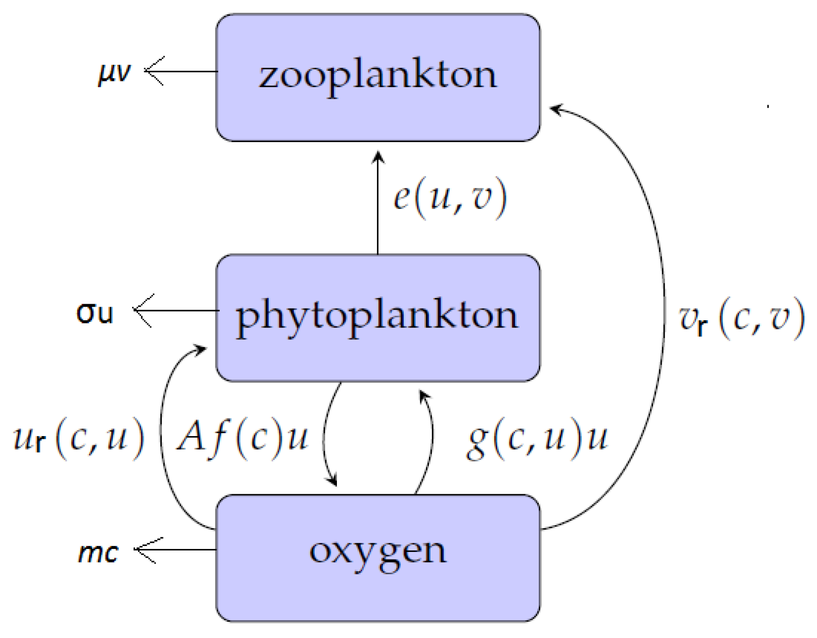
The structure of the model is shown schematically in Figure 1. Flows of matter through the system are indicated by arrows, and the quantification of these flows are given on each arrow respectively. This block-chain model therefore describes the increase in oxygen concentration as a result of photosynthetic activity by phytoplankton. The produced oxygen is consumed in metabolic activities involving respiration for both phytoplankton and zooplankton. Furthermore, phytoplankton is grazed upon by zooplankton. Therefore, the role of zooplankton is twofold: to control phytoplankton density by predation and to consume oxygen through breathing.
We begin with the nonspatial system (for the moment still using the approximation of a well-mixed upper layer) which is described by the following equations [11,12]:
where c is the concentration of the dissolved oxygen, and u and v are the densities of phytoplankton and zooplankton, respectively. The term describes the rate of oxygen production per unit phytoplankton mass where describes the rate of increase in the concentration of the dissolved oxygen due to its transport from phytoplankton cells to the surrounding water and parameter A quantifies the rate of oxygen production inside the cell; A is known to depend on environmental factors such as the availability of sunlight, the availability of CO and the water temperature. The terms and describe, respectively, the rates of the oxygen consumption by the phytoplankton (as required for its metabolism) and zooplankton (as needed for its breathing). The last term in Equation (1) accounts for the losses of oxygen due to its natural depletion (e.g., due to biochemical reactions in the water) with rate m. Function is the per capita phytoplankton growth rate. We consider it to be a function of the oxygen concentration as, apparently, a certain minimum amount of oxygen is needed for the phytoplankton metabolism, and there is biological evidence for that [14]. Function describes the grazing of zooplankton on phytoplankton, i.e., predation. The consumed phytoplankton biomass is transformed into the zooplankton biomass with efficiency ; see the first term in the right-hand side of Equation (3). Since the well-being of zooplankton obviously depends on the oxygen concentration (so that, ultimately, it dies if there is not enough oxygen to breathe), we assume that . The terms and describe the natural mortality of phytoplankton and zooplankton with rates and , respectively.
Using some available data along with relevant biological argument, all functional responses in Equations (1)–(3) can be specified; the details of how such a model is derived are described in detail in a previous publication [12]. Having then introduced dimensionless variables [10,12], we arrive at the following system:
where B and are, respectively, the phytoplankton linear growth rate and the efficiency of the mass turnover in the large oxygen limit (i.e., when oxygen is not a limiting factor), is the competition rate (e.g., due to the self-shading when the plankton density is large), and h, , , , are half-saturation constants. All coefficients are dimensionless. Note that Equations (5) and (6), if considered separately from Equation (4) (hence neglecting oxygen dynamics altogether and keeping the oxygen concentration constant at some hypothetical steady value), coincide with the classical Rosenzweig–McArthur predator-prey model. However, we mention here that a formal reduction of the System (4)–(6) to the two-component phyto-zooplankton model is not possible as cannot give a steady state value of c in case of changing variables u and v.
System (4)–(6) has a few steady states [12]: the extinction state , the coexistence state , and two boundary ‘zooplankton-free’ states and . Whilst the extinction state exists for any parameter value, the nontrivial steady states only exist in a certain parameter range; see [10,12] for details.
Equations (4)–(6) do not contain space. However, in case the water layer is not well mixed, the plankton density and the oxygen concentration become functions of space. In order to make the model spatially explicit, we need to include the transport processes that are responsible for carrying around the system’s components (i.e., oxygen and plankton). Arguably, in the marine environment, the most common and the most powerful of these processes is the turbulent mixing. Having taken its effect in the form of the turbulent diffusion [15], System (4)–(6) turns into the following:
(in dimensionless units) where the turbulent diffusion coefficient is equal to one due to our choice of dimensionless spatial coordinates [12].
Plankton system is affected by several environmental factors. These factors can be physical, i.e., light, temperature, salinity, turbulence etc., or biological such as predation and availability of nutrients [16,17,18,19]. Keeping in mind the possibility to link the change in the dynamics to the effect of the global warming (that can affect the rate of oxygen production) [10,12], we consider the properties of the emerging spatiotemporal patterns subject to the value of the net oxygen production rate A, which we therefore regard as a controlling parameter. In what follows, pattern formation is studied by means of extensive numerical simulations for a different choice of the initial conditions and for a sequence of values of A approaching (and eventually over-passing) the critical value when the sustainable dynamics becomes impossible.
3. Simulation Results: Pattern Formation
Equations (7)–(9) were solved numerically by the finite-differences method in a rectangular domain with and . At the domain boundary, the no-flux Neumann boundary conditions were imposed. Simple explicit scheme was used. It was checked that the choice of the spatial and temporal mesh steps is sufficiently small to avoid any essential numerical artifacts. For simulations, we chose parameter values as , , , , , , , , , and , and vary A over a certain range. Our choice of parameters is based on the previous studies of the corresponding plankton-oxygen model with one spatial dimension [10,12] where it was shown that the above parameter set ensures (up to some restrictions on possible values of A) the sustainable functioning of the system.
Simulations are performed for a few different types of initial conditions. Our first choice of the initial conditions describes spatially homogeneous distributions for both oxygen and phytoplankton at their steady states whilst the zooplankton density is a linear function of space with a very small gradient:
where the values used in simulations are and . We mention here that, based on the properties of some other well-known and similar models (e.g., see [20,21]), the details of the initial species distribution can affect the system’s dynamics at small time but they are unlikely to affect the dynamics at large time, after the transients associated with the initial conditions disappear.
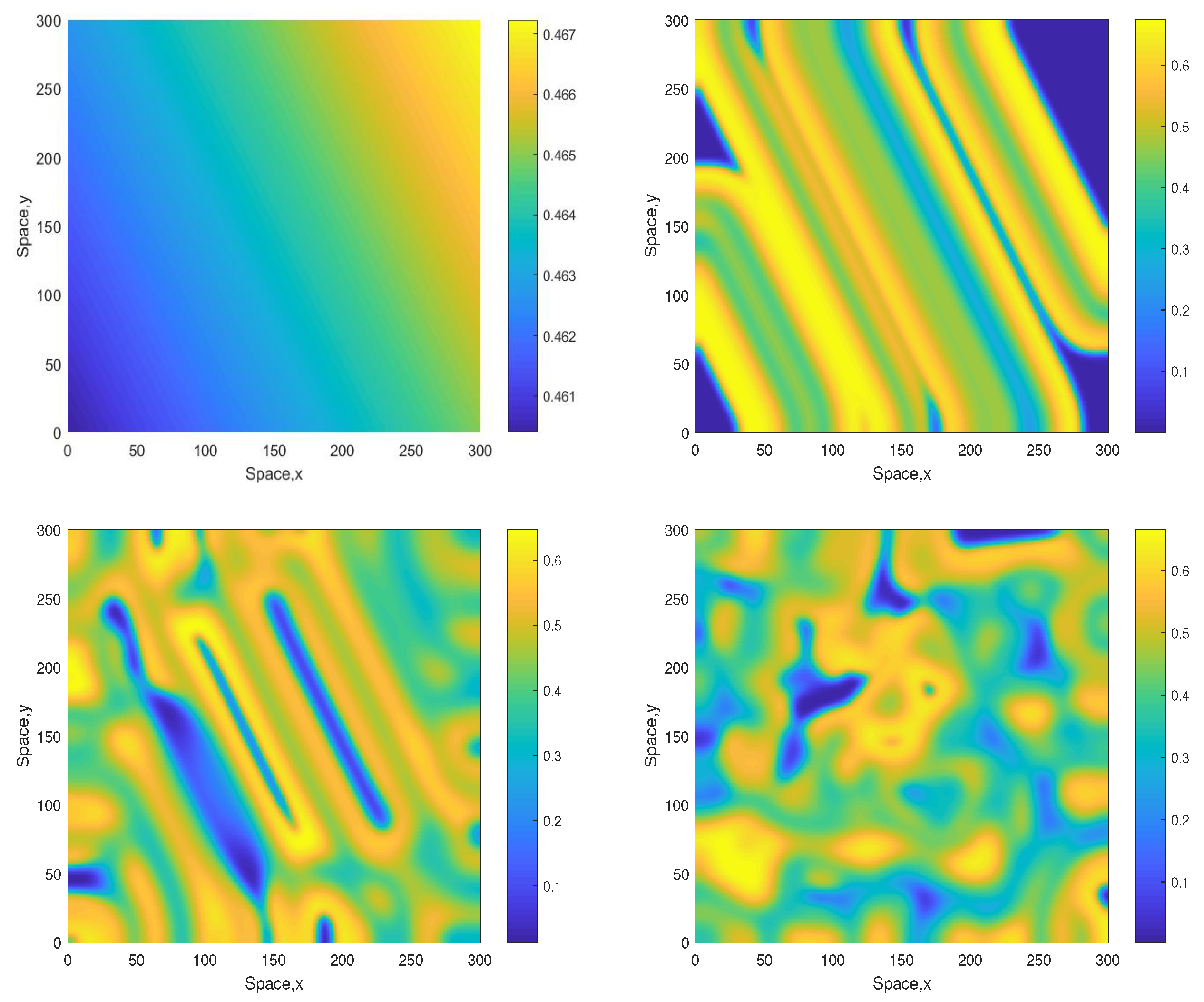
Some snapshots of the system dynamics for the initial conditions given by Equations (10)–(12) are shown in Figure 2 and Figure 3. The distributions of oxygen, phyto- and zooplankton exhibit qualitatively similar behavior, hence only the oxygen concentration is shown. Figure 2 (obtained for ) shows that the evolution of the initial conditions first leads to the formation of stripes. Eventually the stripes are destroyed by the perturbation induced by the boundary resulting, in the large-time limit, in an irregular patchy structure.
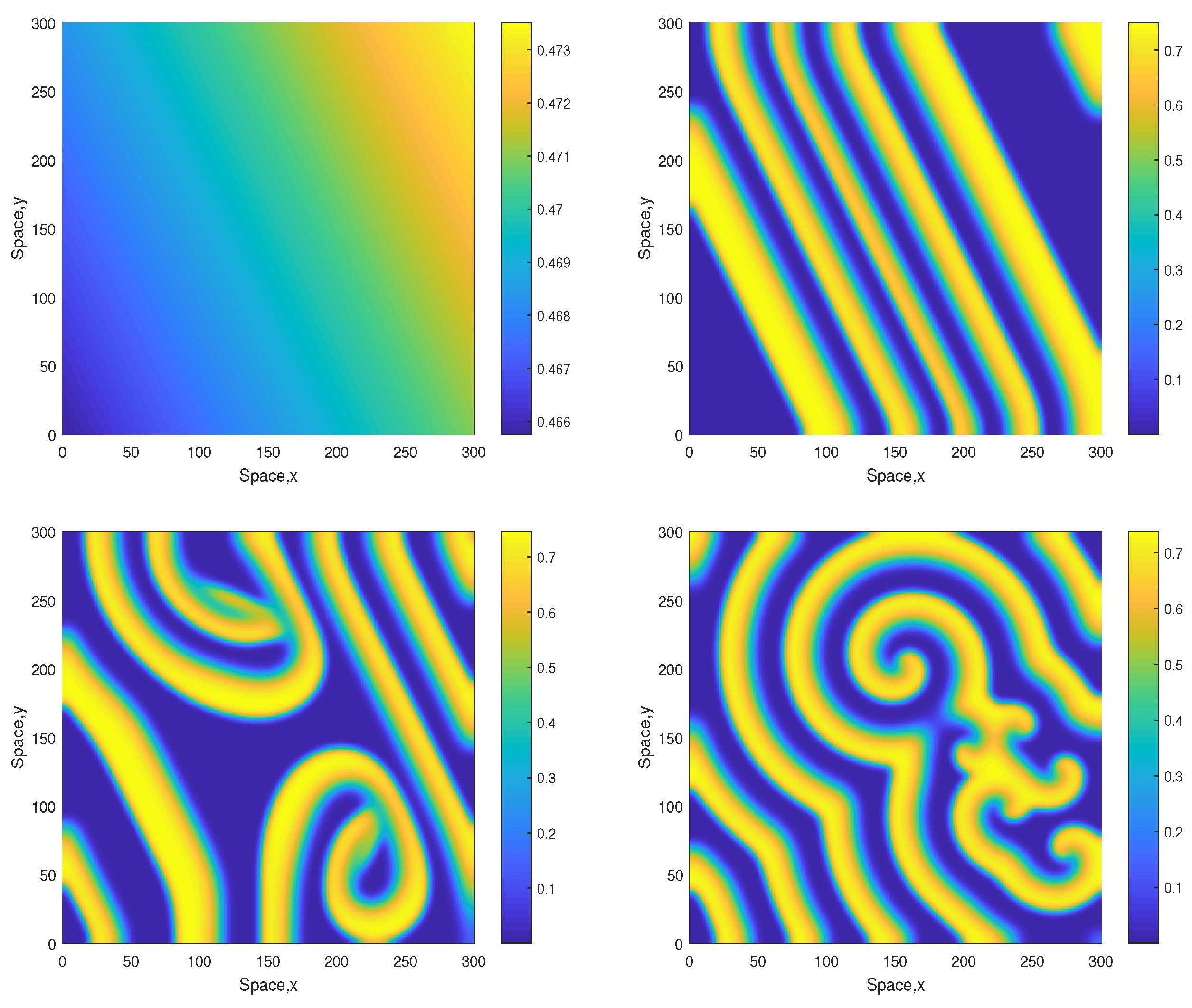
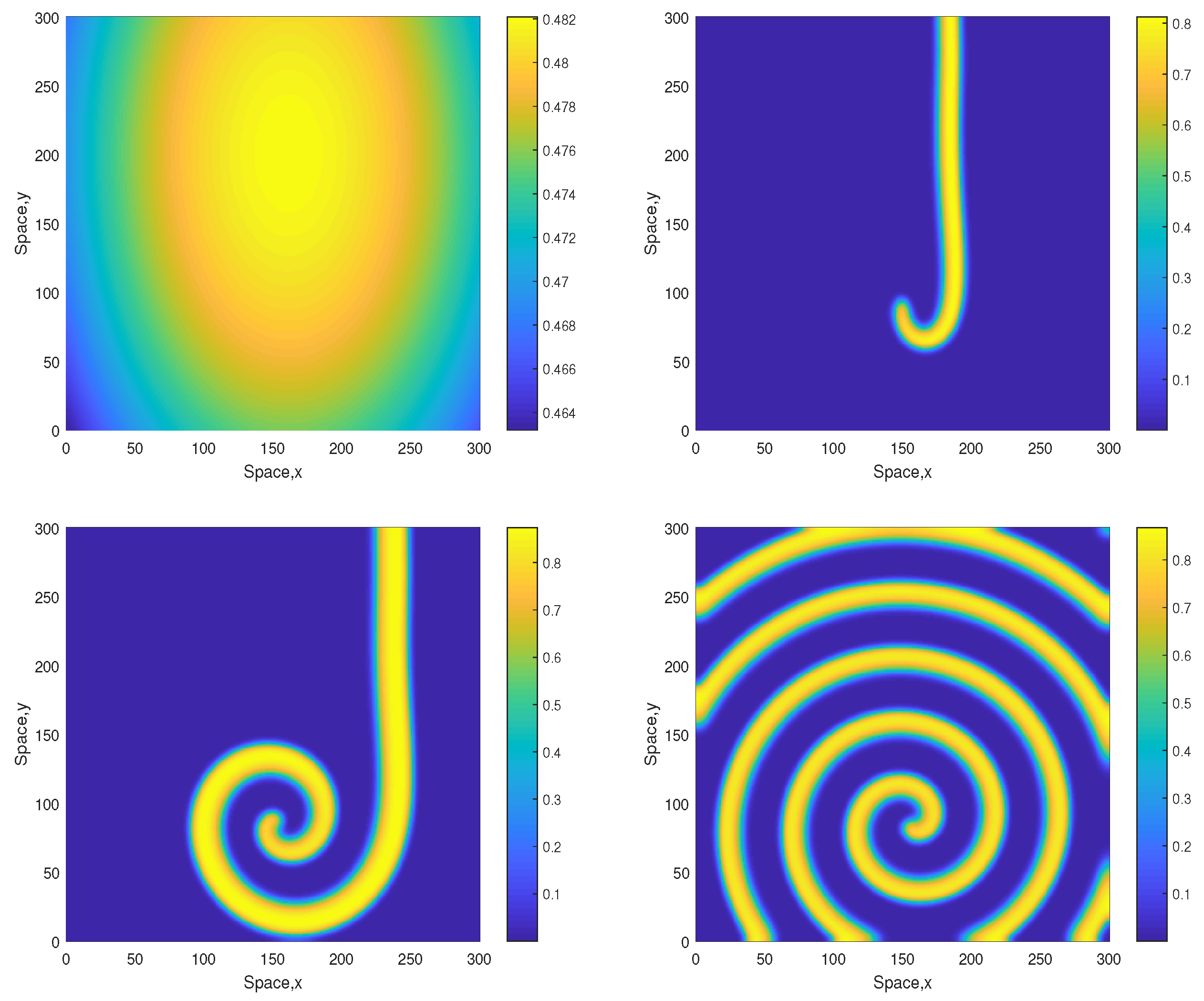
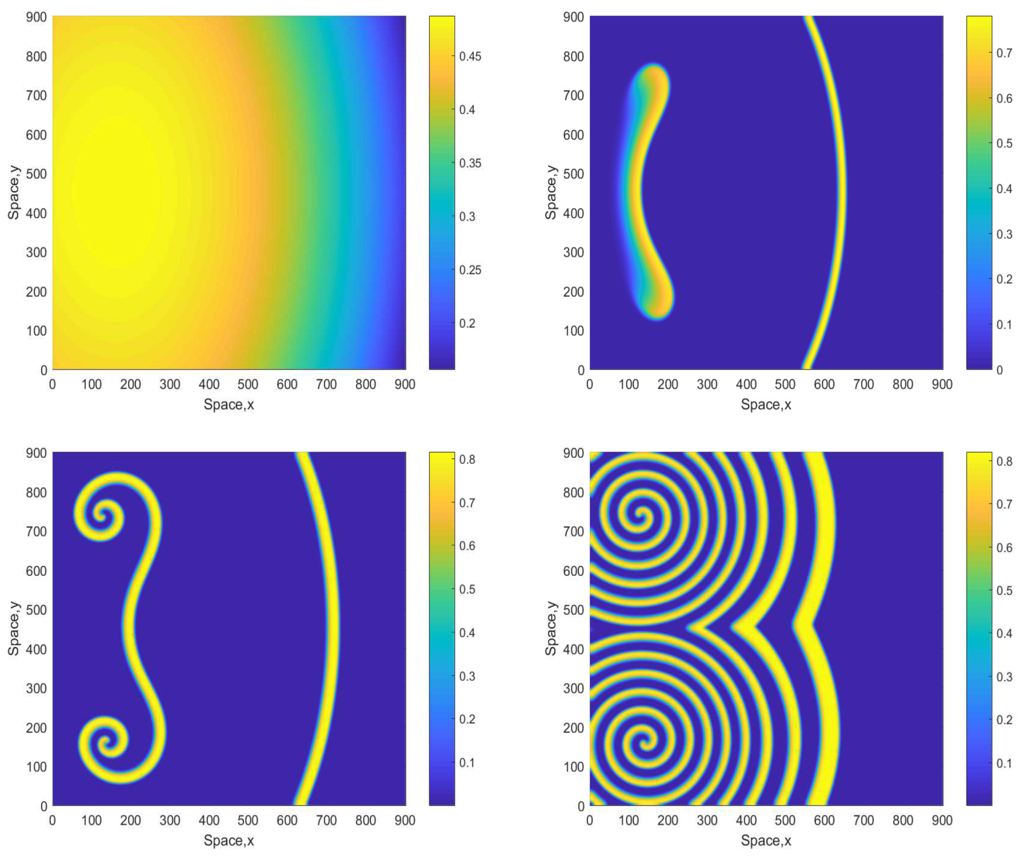
The dynamics become different for a larger value of A. Figure 3 shows snapshots of the oxygen concentration arising from the same initial conditions Equations (10)–(12) but for . In this case, the stripes that emerge at the early stage of dynamics are not being destroyed but evolve to spirals. The spiral pattern appears to be sustainable (which was checked in simulations running up to ) and is not evolving to the patchy structure. We mention here that for this value of A the nonspatial system is unsustainable regardless of the initial conditions (resulting in the oxygen depletion and plankton extinction) [12].
We now consider a different initial condition where only the oxygen concentration is uniform but both the phyto- and zooplankton densities are described by slowly changing functions:
where , and . For these initial conditions, the formation of irregular patchy structure in the large-time limit is shown in Figure 4 (obtained for ). Since in this case the initial conditions are lacking planar symmetry, no stripes are seen at the intermediate time.
However, for a larger value of A the patterns become different showing the same tendency as above, i.e., they become more regular and exhibit a clear spiral structure. A typical example is shown in Figure 5 obtained for . Similar dynamics are observed for some larger values of A, e.g., see Figure 6 obtained for and the same initial conditions given by Equations (13)–(15). The spiral pattern appears to be stable and sustainable as was checked in simulations running up to . Formation of the spirals at large time is preceded by the transient snake-like pattern (cf. the top-right panel in Figure 5 and Figure 6). We want to emphasize that, for values , the corresponding 1D system is not sustainable and the evolution of initial distributions promptly leads to the oxygen depletion and the plankton extinction [12]. (Here we also recall that the corresponding nonspatial system becomes unsustainable already for , see [12].) Therefore, the higher persistence of the system observed in the 2D case should be attributed solely to the effect of the pattern formation.
Now we are going to check whether the results obtained above are sensitive to the size of the domain and to a further modification of the initial distributions. We therefore perform simulations in a larger domain for the following initial conditions:
where , and have the same values as in (13)–(15).
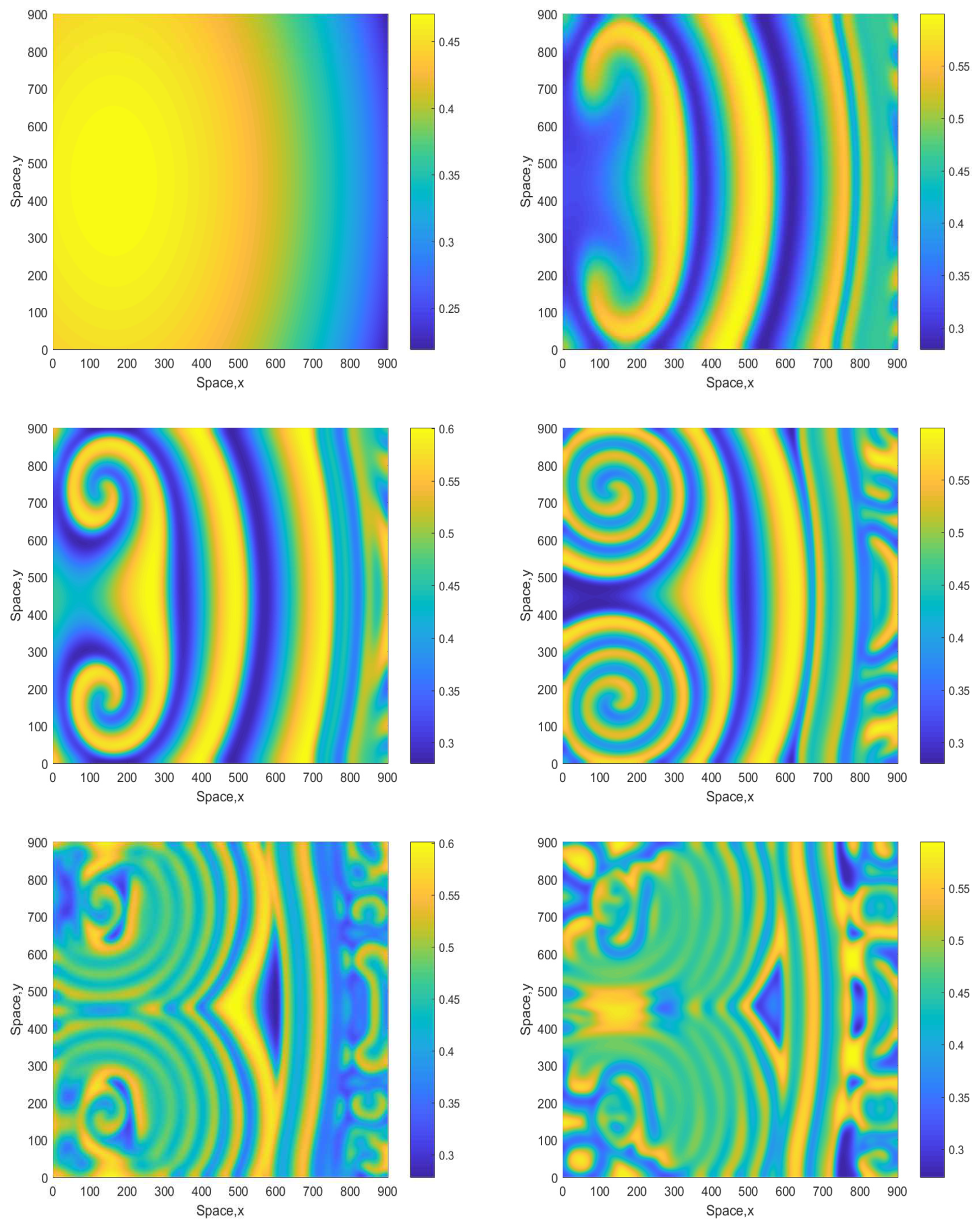
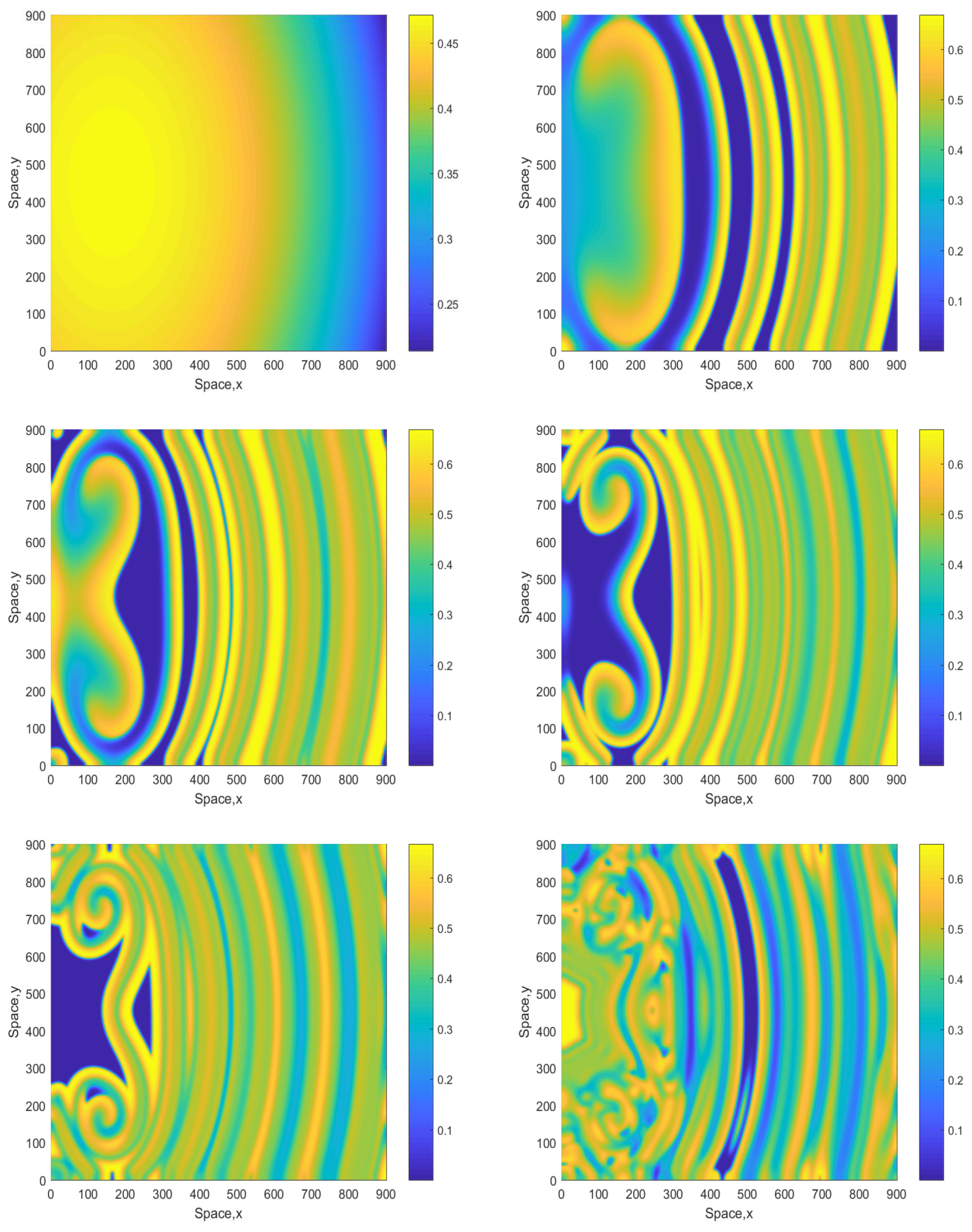
Figure 7 shows snapshots of the oxygen concentration obtained for and the initial conditions given by Equations (16)–(18). We observe that, in the large time run, the system eventually evolves to an irregular patchy distribution similar to the ones shown in the bottom-right panel in Figure 2 and Figure 4. There are, however, some differences: in the case shown in Figure 7 (middle row), the irregular patchy pattern is preceded by the formation of a double spiral or a “mushroom-like” structure. For a somewhat larger value of A, the dynamics exhibits similar features (see Figure 8 obtained for ) except for the relatively minor difference that the spirals are of a different shape and that for the intermediate time the spatial distribution is becoming more prominently heterogeneous, cf. the dark-blue areas in the middle and bottom rows of Figure 8 and the range of values on the color bar.
An increase in A results in a change in the emerging pattern similar to what was observed in the smaller domain (cf. Figure 2 and Figure 3), i.e., the evolution of the initial conditions leads to the formation of a clear spiral pattern, see Figure 9 obtained for and the initial conditions given by Equations (13)–(15). The pattern is stable and sustainable and does not evolve into an irregular or patchy distribution; this was checked in simulations running up to 15,000.
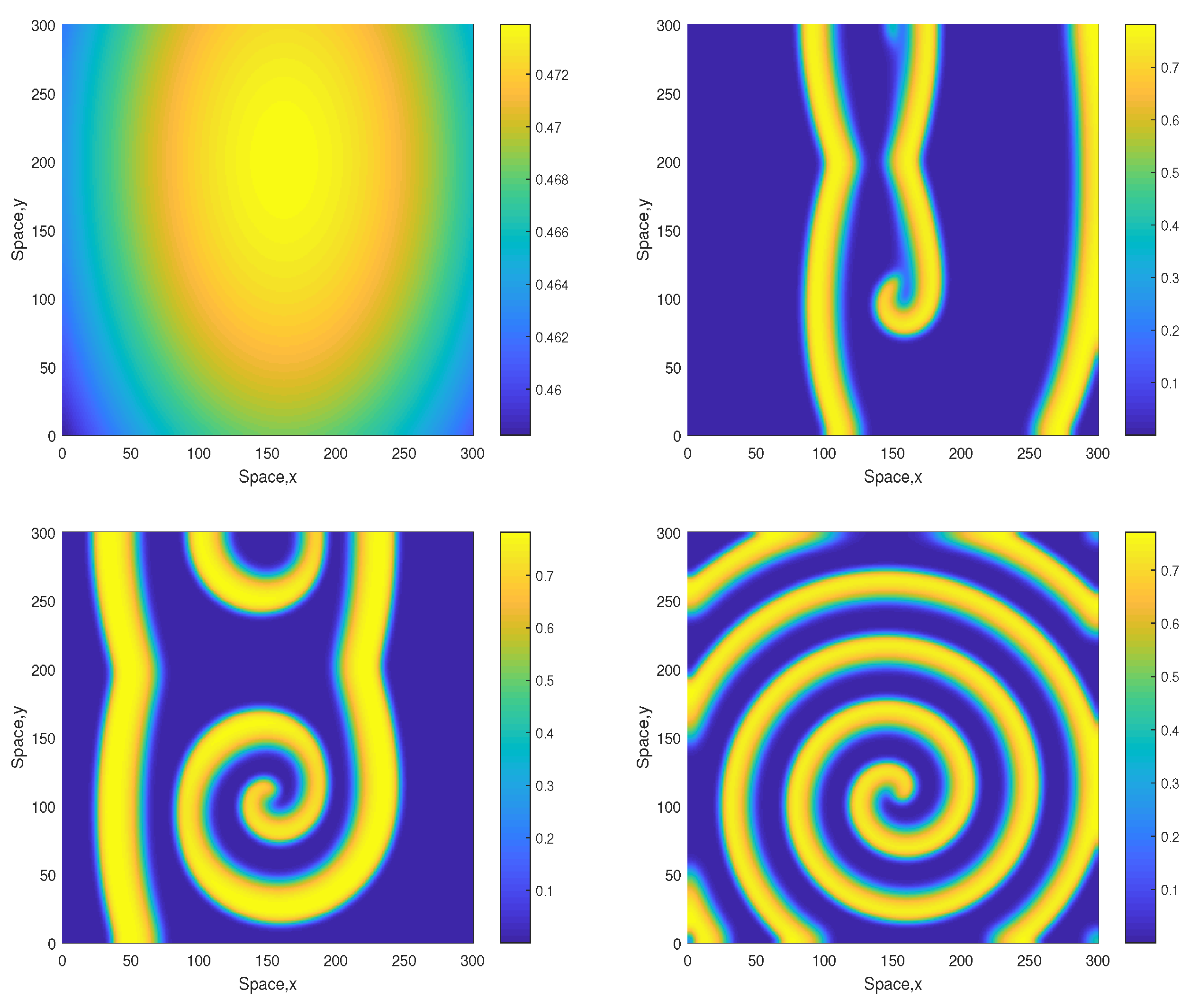
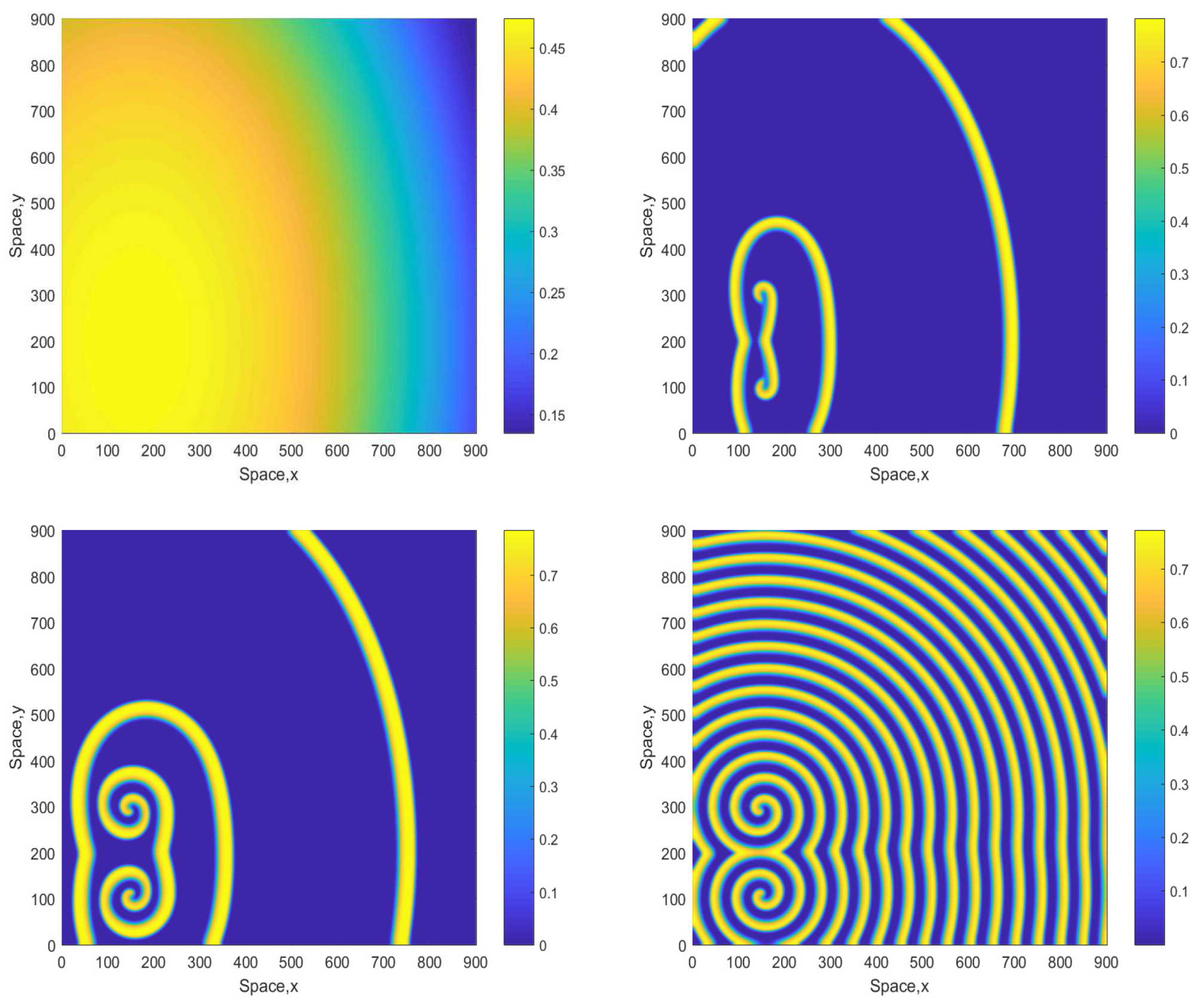
A further increase in A to somewhat larger values (up to about ) does not change the dynamics in a significant way but can make the spirals or mushroom-like patterns be seen more clearly at already smaller time. Figure 10 shows snapshots of the oxygen concentration obtained for . The evolution of the initial conditions first leads to a zigzag, mushroom-like structure (already at ) from which a clear double spiral eventually develops. The double spiral is stable and sustainable and is not further evolving to a distribution with different properties (e.g., patchy) as was checked in long-run simulations.
Once again, we notice that the persistent spatial patterns shown in Figure 9 and Figure 10 exist in the parameter range where the system becomes unsustainable in the corresponding 1D case (i.e., for ). We therefore consistently observe that the dynamics of the 2D system is sustainable in a broader parameter range. However, a much larger increase in A (approximately up to 3.5 or larger) will make the 2D system non-viable too, resulting in plankton extinction and oxygen depletion.
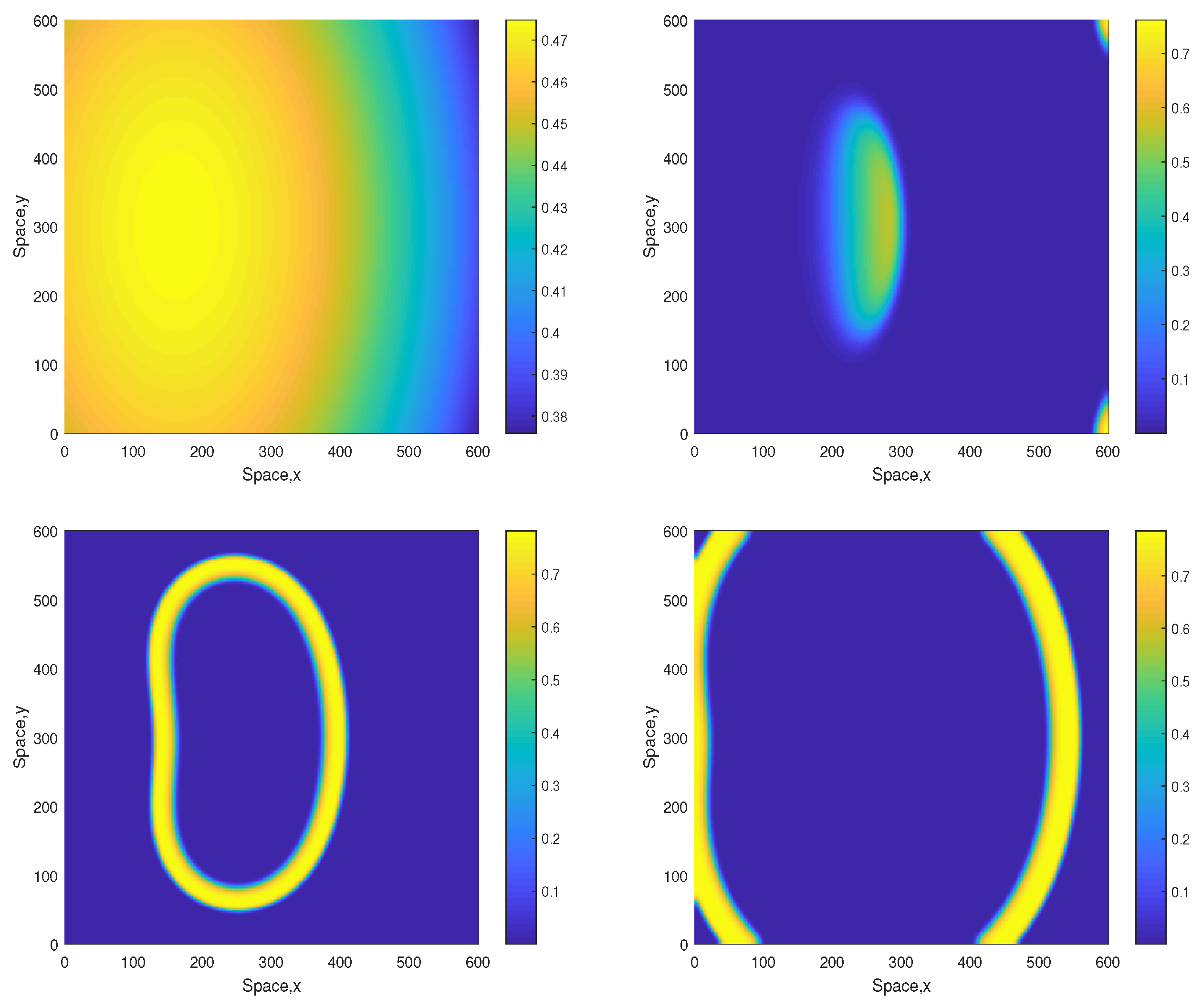
We also notice that in the parameter range where the dynamics is only sustainable in a higher-dimensional system (e.g., 2D vs. 1D), the dynamics becomes more sensitive to the details of the initial conditions. For a given parameter set, whilst one choice of the initial distributions would evolve to a sustainable spiral pattern, another choice might eventually lead to extinction. One example is shown in Figure 11. The evolution of the initial distributions leads to the formation of a ring-like elliptic shape. The shape then grows in size hence ‘propagating’ through the space towards the domain boundaries. Outside and inside the ring, the oxygen concentration and the plankton densities are close to zero. Eventually the ring collides with the boundary and disappears, thus resulting in the system collapse (extinction and depletion).
4. Discussion and Concluding Remarks
Dynamics of the dissolved oxygen in the ocean has been attracting considerable attention over the last decade [8,9,22,23,24]. The existing observations point out at a gradual decrease of the average oxygen level across the globe, with the areas of extreme conditions (a severe lack of oxygen resulting in anoxia and mass mortality of the marine fauna) being fast growing in size. Although there is a consensus that the oxygen decrease is a result of global climate change, in particular global warming, the specific reasons and mechanisms of the decrease remain controversial. The decrease was previously linked to purely physical mechanisms such as the decrease of oxygen solvability in warmer waters [23,24]. More recently, however, it was shown that global warming can significantly affect the amount of dissolved oxygen also through a biological mechanism as it can disrupt the oxygen production by phytoplankton potentially leading to global ocean anoxia [10,12,25]. Moreover, since it is estimated that about 70% of the atmospheric oxygen is produced in the ocean, such a global disruption of oxygen production would eventually lead to a significant decrease of the oxygen concentration in the air and could hence lead to mass mortality of animals and humans.
In our previous work, the above issue was addressed theoretically using a novel mathematical model of the coupled plankton-oxygen dynamics and extensive computer simulations [11,12]. However, the specific focus was on the dynamics of non-spatial (“well-mixed”) system and the system with one spatial dimension. For the nonspatial system, it was shown that the sustainable dynamics is only possible when the oxygen production rate (i.e., A) is in an intermediate range, i.e., not too high and not too low [10,12]. Interestingly, it was shown that the corresponding 1D spatial system exhibits similar properties but the parameter range of sustainable dynamics is somewhat broader. Therefore, the question arises as to whether the sustainability range may be even broader in a more realistic 2D system (i.e., system with two spatial dimensions) or perhaps the oxygen depletion catastrophe would not happen at all. Indeed, there are many examples in theoretical ecology where the 2D system is sustainable whilst the corresponding 1D or nonspatial systems are not; e.g., see Chapter 12 in [20].
In this paper, we have considered the above question using the 2D spatially-explicit model of the plankton-oxygen dynamics; see Equations (7)–(9). Our main focus is on the pattern formation as it is well known from other population dynamics models that pattern formation can enhance system’s sustainability [20]. Since our ultimate goal is to put our results into the context of global warming (cf. [10,12]), we use A as the controlling parameter as there is significant biological evidence that the rate of net oxygen production depends on the water temperature [26,27,28,29]. Using extensive numerical simulations, we have shown that the model exhibits rich spatiotemporal dynamics. In the parameter range where the nonspatial system either possesses a stable limit cycle or becomes non-sustainable when the cycle is destroyed in a non-local bifurcation (see [10] for details), the evolution of the initial conditions leads to the formation of spatiotemporal patterns. In particular, we have observed (for somewhat different initial conditions) irregular spatiotemporal patterns, simple spirals, double spirals or “mushroom-like” structures, and “snake-like” structures. Here we recall that the spatial distribution of the dissolved oxygen typically shows a patchy structure [8,9], although the quality of the available data (e.g., the spatial resolution) does not make it possible to look into the details of that structure. Whilst quantitative comparison between theory and data lies beyond the scope of this paper, we conclude that our results are in qualitative agreement with at least some of the field data. We also mention here that spiral-like and mushroom-like spatial plankton patterns are frequently observed in the ocean [30,31]. Mushroom structures are usually linked to particular hydrodynamical conditions (e.g., the meeting of two masses of water, one cold and the other warm, cf. [30]); the results of our study apparently suggest an alternative explanation where the formation of such structures mostly results from biological interactions.
Interestingly, the type of the pattern depends on A. Whilst a value of A taken in the middle of the sustainable range results in a nearly-uniform oxygen and plankton distribution, for larger values of A normally lead to spatially irregular, strongly heterogeneous, large-amplitude patterns. Along with a further increase in A, patterns tend to become more regular. For a sufficiently large value of A, the depletion of oxygen and the plankton extinction (which can be preceded by long living spiral patterns) is the only issue, similar to what was observed in the corresponding 1D and nonspatial models. The value of A for which the extinction is observed appears to be slightly larger than it is in the 1D case.
We also notice that for larger values of A—i.e., the values that are close to the sustainable parameter range—the spiral or double-spiral patterns appear to be typical. This seems to suggest that the emergence of spirals in the spatial distributions of the oxygen concentration can be regarded as an early warning signal of the approaching tipping point.
Our study leaves a few open questions. In this paper we considered the two spatial dimensions with no spatial structure, which arguably corresponds to the horizontal coordinates. This seems to be a natural extension of the 1D case. An interesting alternative could be a 2D model describing the vertical distribution of oxygen and plankton, i.e., where one spatial coordinate would correspond to the depth. Such a model should include an explicit dependence on the vertical coordinate in order to account for the ocean stratification. One can expect that such a system could have rather different properties.
Note that in this paper our goal is to reveal some generic scenarios of pattern formation as it helps to understand the limits of the system’s sustainability and also to identify possible early warning signals of the approaching tipping point. For this purpose, dimensionless variables and parameters are sufficient. However, in order to make the study more quantitative and to eventually compare our predictions to field or laboratory data and, ultimately, to increase the model’s predictive power, the results should be presented using the original, dimensional physical/biological units. Technically, it is easy to do using the definition of the dimensionless variables—as soon as all the original parameters are known. The latter, however, is a challenging task and requires much more than routine work as the value of most of the parameters is known with a low precision, sometimes only up to an order of magnitude. Making a careful and sensible analysis of the available empirical data to translate our results to the real, dimensional units lies beyond the scope of this paper and but will become a focus of future work.
Another open issue is the description of the turbulent transport. Although the turbulent diffusion framework is a widely used approach, it has its limitations, especially in a multiscale, fully developed turbulent flow. One alternative framework is based on the theory of chaotic flows [32]. Several studies on the population dynamics in marine ecosystems [33,34] used this framework and showed that its predictions can be different from those obtained using the turbulent diffusion approach. Extending our model of the coupled plankton-oxygen dynamics to better describe the properties of the turbulent mixing is a challenge for future work.
Author Contributions
S.P. designed the research. Y.S. wrote the numerical code and performed simulations. S.P. and Y.S. wrote the manuscript.
Funding
This research received no external funding.
Conflicts of Interest
The authors declare no conflicts of interest.
References
- Allegretto, W.; Mocenni, C.; Vicino, A. Periodic solutions in modelling lagoon ecological interactions. J. Math. Biol. 2005, 51, 367–388. [Google Scholar] [CrossRef] [PubMed]
- Hull, V.; Mocenni, C.; Falcucci, M.; Marchettini, N. A trophodynamic model for the lagoon of Fogliano (Italy) with ecological dependent modifying parameters. Ecol. Model. 2000, 134, 153–167. [Google Scholar] [CrossRef]
- Hull, V.; Parrella, L.; Falcucci, M. Modelling dissolved oxygen dynamics in coastal lagoons. Ecol. Model. 2008, 211, 468–480. [Google Scholar] [CrossRef]
- Marchettini, N.; Mocenni, C.; Vicino, A. Integrating slow and fast dynamics in a shallow water coastal lagoon. Ann. Di Chim. 1999, 89, 505–514. [Google Scholar]
- Misra, A. Modeling the depletion of dissolved oxygen in a lake due to submerged macrophytes. Nonlinear Anal. Model. Control 2010, 15, 185–198. [Google Scholar]
- Misra, A.K.; Chandra, P.V.; Raghavendra, V. Modeling the depletion of dissolved oxygen in a lake due to algal bloom: Effect of time delay. Adv. Water Resour. 2011, 34, 1232–1238. [Google Scholar] [CrossRef]
- Caruso, A.; Gargano, M.E.; Valenti, D.; Fiasconaro, A.; Spagnolo, B. Cyclic fluctuations, climatic changes and role of noise in Planktonic Foraminifera in the Mediterranean Sea. Fluct. Noise Lett. 2005, 5, L349–L355. [Google Scholar] [CrossRef]
- Ito, T.; Minobe, S.; Long, M.C.; Deutsch, C. Upper ocean O2 trends: 1958–2015. Geophys. Res. Lett. 2017, 44, 4214–4223. [Google Scholar] [CrossRef]
- Richardson, K.; Bendtsen, J. Photosynthetic oxygen production in a warmer ocean: The Sargasso Sea as a case study. Phil. Trans. R. Soc. A 2017, 375. [Google Scholar] [CrossRef] [PubMed]
- Petrovskii, S.; Sekerci, Y.; Venturino, E. Regime shifts and ecological catastrophes in a model of plankton-oxygen dynamics under the climate change. J. Theor. Biol. 2017, 424, 91–109. [Google Scholar] [CrossRef] [PubMed]
- Sekerci, Y.; Petrovskii, S. Mathematical modelling of spatiotemporal dynamics of oxygen in a plankton system. Math. Model. Nat. Phenom. 2015, 10, 96–114. [Google Scholar] [CrossRef]
- Sekerci, Y.; Petrovskii, S. Mathematical modelling of plankton–oxygen dynamics under the climate change. Bull. Math. Biol. 2015, 77, 2325–2353. [Google Scholar] [CrossRef] [PubMed]
- Conte, F.; Cubbage, J. Phytoplankton and recreational ponds. West. Reg. Aquacult. Center 2001, 5, 1–6. [Google Scholar]
- Franke, U.; Hutter, K.; Jöhnk, K. A physical-biological coupled model for algal dynamics in lakes. Bull. Math. Biol. 1999, 61, 239–272. [Google Scholar] [CrossRef] [PubMed]
- Okubo, A. Diffusion and ecological problems: Mathematical models. In Biomathematics; Springer: Berlin, Germany, 1980; Volume 10. [Google Scholar]
- Abbott, M.R. Phytoplankton patchiness: Ecological implications and observation methods. Patch Dyn. 1993, 96, 37–49. [Google Scholar]
- Denman, K.L. Covariability of chlorophyll and temperature in the sea. In Deep Sea Research and Oceanographic Abstracts; Elsevier: Amsterdam, The Netherlands, 1976; Volume 23, pp. 539–550. [Google Scholar]
- Fasham, M. The statistical and mathematical analysis of plankton patchiness. Oceanogr. Mar. Biol. Annu. Rev. 1978, 16, 43–79. [Google Scholar]
- Platt, T. Local phytoplankton abundance and turbulence. Deep Sea Res. Oceanogr. Abstr. 1972, 19, 183–187. [Google Scholar] [CrossRef]
- Malchow, H.; Petrovskii, S.V.; Venturino, E. Spatiotemporal Patterns in Ecology and Epidemiology: Theory, Models, and Simulation; Chapman & Hall/CRC Press: London, UK, 2008. [Google Scholar]
- Medvinsky, A.B.; Petrovskii, S.V.; Tikhonova, I.A.; Malchow, H.; Li, B.-L. Spatiotemporal complexity of plankton and fish dynamics. SIAM Rev. 2002, 44, 311–370. [Google Scholar] [CrossRef]
- Battaglia, G.; Joos, F. Hazards of decreasing marine oxygen: The near-term and millennial-scale benefits of meeting the Paris climate targets. Earth Syst. Dyn. Discuss. 2017. [Google Scholar] [CrossRef]
- Breitburg, D.; Levin, L.A.; Oschlies, A.; Grégoire, M.; Chavez, F.P.; Conley, D.J.; Garçon, V.; Gilbert, D.; Gutiérrez, D.; Isensee, K.; et al. Declining oxygen in the global ocean and coastal waters. Science 2018, 359, eaam7240. [Google Scholar] [CrossRef] [PubMed]
- Shaffer, G.; Olsen, S.M.; Pedersen, J.O.P. Long-term ocean oxygen depletion in response to carbon dioxide emissions from fossil fuels. Nat. Geosci. 2009, 2, 105–109. [Google Scholar] [CrossRef]
- Sekerci, Y.; Petrovskii, S.V. Global warming can lead to depletion of oxygen by disrupting phytoplankton photosynthesis: A mathematical modelling approach. Geosciences 2018, 8, 201. [Google Scholar] [CrossRef]
- Hancke, K.; Glud, R.N. Temperature effects on respiration and photosynthesis in three diatom-dominated benthic communities. Aquat. Microb. Ecol. 2004, 37, 265–281. [Google Scholar] [CrossRef] [Green Version]
- López-Sandoval, D.C.; Rodriguez-Ramos, T.; Cermeño, P.; Sobrino, C.; Marañón, E. Photosynthesis and respiration in marine phytoplankton: Relationship with cell size, taxonomic affiliation, and growth phase. J. Exp. Mar. Biol. Ecol. 2014, 457, 151–159. [Google Scholar] [CrossRef]
- McKinnon, A.D.; Duggan, S.; Logan, M.; Lonborg, C. Plankton respiration, production, and trophic state in tropical coastal and shelf waters adjacent to Northern Australia. Front. Mar. Sci. 2017, 4, 346. [Google Scholar] [CrossRef]
- Robinson, C. Plankton gross production and respiration in the shallow water hydrothermal systems of Milos, Aegean Sea. J. Plankt. Res. 2000, 22, 887–906. [Google Scholar] [CrossRef] [Green Version]
- Bardey, P.; Garnesson, P.; Moussu, G.; Wald, L. Joint analysis of temperature and ocean colour satellite images for mesoscale activities in the Gulf of Biscay. Int. J. Remote Sens. 1999, 20, 1329–1341. [Google Scholar] [CrossRef]
- Wyatt, T. The biology of Oikopleura dioica and Fritillaria borealis in the southern bight. Mar. Biol. 1973, 22, 137–158. [Google Scholar] [CrossRef]
- Neufeld, Z.; Tel, T. Advection in chaotically time-dependent open flows. Phys. Rev. E 1998, 57, 2832–2842. [Google Scholar] [CrossRef] [Green Version]
- Bracco, A.; Provenzale, A.; Scheuring, I. Mesoscale vortices and the paradox of the plankton. Proc. R. Soc. Ser. B 2000, 267, 1795–1800. [Google Scholar] [CrossRef] [PubMed] [Green Version]
- Károlyi, G.; Péntek, A.; Scheuring, I.; Tél, T.; Toroczkai, Z. Chaotic flow: The physics of species coexistence. Proc. Natl. Acad. Sci. USA 2000, 97, 13661–13665. [Google Scholar] [CrossRef] [PubMed] [Green Version]
Figure 1.
The structure of the conceptual model describing the interactions between oxygen (c), phytoplankton (u) and zooplankton (v). Arrows show the flows of matter through the system, and the parameterizations of the rates are as labelled. Phytoplankton produces oxygen through photosynthesis during the day-time then consumes it during the night [13]. Zooplankton feeds on phytoplankton and consumes oxygen through breathing; see further details in the text.

Figure 2.
Snapshots of the oxygen spatial distribution obtained for and shown for for , , and (left to right, top to bottom), other parameters are given in the text. The initial conditions are given by Equations (10)–(12) where , and .
Figure 2.
Snapshots of the oxygen spatial distribution obtained for and shown for for , , and (left to right, top to bottom), other parameters are given in the text. The initial conditions are given by Equations (10)–(12) where , and .

Figure 3.
Spatial distribution of the oxygen concentration obtained for and shown for , , and (left to right, top to bottom). Other parameters are the same as above. The initial conditions are given by Equations (10)–(15) with , and .
Figure 3.
Spatial distribution of the oxygen concentration obtained for and shown for , , and (left to right, top to bottom). Other parameters are the same as above. The initial conditions are given by Equations (10)–(15) with , and .

Figure 4.
Spatial distribution of the oxygen concentration obtained for and shown for , , and (left to right, top to bottom). Other parameters are the same as above. The initial conditions are given by Equations (13)–(15) with , and .
Figure 4.
Spatial distribution of the oxygen concentration obtained for and shown for , , and (left to right, top to bottom). Other parameters are the same as above. The initial conditions are given by Equations (13)–(15) with , and .

Figure 5.
Spatial distribution of the oxygen concentration obtained for and shown for , , and (left to right, top to bottom). Other parameters are the same as above. The initial conditions are given by Equations (13)–(15) with , and .
Figure 5.
Spatial distribution of the oxygen concentration obtained for and shown for , , and (left to right, top to bottom). Other parameters are the same as above. The initial conditions are given by Equations (13)–(15) with , and .

Figure 6.
Spatial distribution of the oxygen concentration obtained for and shown for , , and (left to right, top to bottom). Other parameters are the same as above. The initial conditions are given by Equations (13)–(15) with , and .
Figure 6.
Spatial distribution of the oxygen concentration obtained for and shown for , , and (left to right, top to bottom). Other parameters are the same as above. The initial conditions are given by Equations (13)–(15) with , and .

Figure 7.
Spatial distribution of the oxygen concentration obtained for in a larger domain and shown for , , , , and (left to right, top to bottom). Other parameters are the same as above. The initial conditions are given by Equations (16)–(18) with , and .
Figure 7.
Spatial distribution of the oxygen concentration obtained for in a larger domain and shown for , , , , and (left to right, top to bottom). Other parameters are the same as above. The initial conditions are given by Equations (16)–(18) with , and .

Figure 8.
Spatial distribution of the oxygen concentration obtained for and shown for , , , , and (left to right, top to bottom). Other parameters and the initial conditions are the same as in Figure 7.
Figure 8.
Spatial distribution of the oxygen concentration obtained for and shown for , , , , and (left to right, top to bottom). Other parameters and the initial conditions are the same as in Figure 7.

Figure 9.
Spatial distribution of the oxygen concentration obtained for and shown for , , and (left to right, top to bottom). The other parameters are the same as above. The initial conditions are given by Equations (13)–(15) with , .
Figure 9.
Spatial distribution of the oxygen concentration obtained for and shown for , , and (left to right, top to bottom). The other parameters are the same as above. The initial conditions are given by Equations (13)–(15) with , .

Figure 10.
Spatial distribution of the oxygen concentration obtained for and shown for , , and (left to right, top to bottom). Other parameters are the same as above. The initial conditions are given by Equations (16)–(18) with , and .
Figure 10.
Spatial distribution of the oxygen concentration obtained for and shown for , , and (left to right, top to bottom). Other parameters are the same as above. The initial conditions are given by Equations (16)–(18) with , and .

Figure 11.
Spatial distribution of the oxygen concentration in computational domain obtained for and shown for , , and (left to right, top to bottom). Note that all parameters are the same as in Figure 5, but the initial conditions are slightly different, i.e., , and . Contrary to the case shown in Figure 5, now the evolution of the initial conditions results in oxygen depletion and species extinction.

© 2018 by the authors. Licensee MDPI, Basel, Switzerland. This article is an open access article distributed under the terms and conditions of the Creative Commons Attribution (CC BY) license (http://creativecommons.org/licenses/by/4.0/).
Share and Cite
MDPI and ACS Style
Sekerci, Y.; Petrovskii, S. Pattern Formation in a Model Oxygen-Plankton System. Computation 2018, 6, 59. https://0-doi-org.brum.beds.ac.uk/10.3390/computation6040059
AMA Style
Sekerci Y, Petrovskii S. Pattern Formation in a Model Oxygen-Plankton System. Computation. 2018; 6(4):59. https://0-doi-org.brum.beds.ac.uk/10.3390/computation6040059
Chicago/Turabian StyleSekerci, Yadigar, and Sergei Petrovskii. 2018. "Pattern Formation in a Model Oxygen-Plankton System" Computation 6, no. 4: 59. https://0-doi-org.brum.beds.ac.uk/10.3390/computation6040059
Note that from the first issue of 2016, this journal uses article numbers instead of page numbers. See further details here.