Article

Mode Pressure Coefficient Maps as an Alternative to Mean Pressure Coefficient Maps for Non-Gaussian Processes: Hyperbolic Paraboloid Roofs as Cases of Study

Department of Engineering and Geology, G. D’Annunzio University, viale Pindaro 42, 65127 Pescara, Italy
Submission received: 9 November 2018 / Revised: 29 November 2018 / Accepted: 10 December 2018 / Published: 12 December 2018
(This article belongs to the Special Issue Computational Methods in Wind Engineering)

Abstract

:
Wind tunnel experiments are necessary for geometries that are not investigated by codes or that are not generally and parametrically investigated by literature. One example is the hyperbolic parabolic shape mostly used for cable net roofs, for which codes do not provide pressure coefficients and literature only gives mean, maxima, and minima pressure coefficient maps. However, most of pressure series acquired in wind tunnels on the roof are not Gaussian processes and, for this reason, the mean values are not precisely representative of the process. The paper investigates the ratio between mean and mode of pressure coefficient series acquired in wind tunnels on buildings covered with hyperbolic paraboloid roofs with square plans. Mode pressure coefficient maps are given as an addition to traditional pressure coefficient maps.

1. Introduction

Wind tunnel tests are necessary for structure sensitivity to wind action regarding shapes not discussed in technical codes or literature. This is the case of the structures with hyperbolic paraboloid shapes mostly used for roofs made of cable nets and concrete shells, widely used, for example, in sport arenas, meeting rooms, or music halls [1,2,3,4]. The shortcoming relates the generalization and parametrization of aerodynamic coefficients to the widest number of geometries derived from the hyperbolic paraboloid.
Codes of practice, such as those found in the literature [5,6,7,8,9,10,11,12,13,14], for example, do not give values of pressure coefficients for buildings covered with hyperbolic paraboloid roofs.
The literature discusses a great number of examples of wind tunnel test campaigns [11,15,16,17,18,19,20,21,22,23,24,25,26,27,28,29,30,31,32]. However, all references regard particular cases that are not generalizable for different geometries.
There are some exceptions [26,27] that have followed a parametric approach in order to give generalizable values. In addition, the authors of [33,34] have synthetized experimental results in order to give simplified pressure coefficient maps.
The simplified pressure coefficient maps are used by designers to calculate the structure and evaluate the cost–benefit convenience in advance.
All publications and codes give mean or maxima and minima pressure coefficient maps. The maxima and minima pressure coefficients are usually considered to estimate the local extreme values of wind action, whereas the mean values are used to investigate the global wind action distribution on the surface.
However, some information about the processes that have been used to generate the maps should be given too.
In fact, if the processes are non-Gaussian, the mean value is not precise enough to represent them. The non-Gaussianity generally depends on very big flow fluctuation because of, for example, flow separation near edges or vortex shedding caused by a complex geometry [27,35]. Recently, the authors of [35,36] illustrated the peak factor distributions on a hyperbolic paraboloid roof and showed that many processes acquired by pressure taps, particularly near the roof borders and corners, are non-Gaussian processes. For these reasons, the mean values of the pressure coefficient series are representative as much as the mode, for example.
In cases where the difference between mean and mode values is significant, if the mean is lower than the mode (i.e., which is the most frequent value), the use of mean pressure coefficients can affect structure reliability. In particular, this variation can affect the structural reliability for flexible structures and in general for cables structures. In fact, analyses of instability on tensile structures, in particular on suspended bridges under flutter (i.e., [37,38,39]), have shown that smaller variations of wind action can also give global instability, contrary to the case of concrete bridges, which are more sensitive to seismic action [40]. In addition, the cable net tensile structures’ sensitivity to wind action is well-known from many studies [1,2,23,41,42,43,44,45,46,47,48,49,50,51,52].
This paper investigates this aspect on four geometries of buildings covered with hyperbolic paraboloid roofs with square plans. This shape was chosen because it is frequently used for tensile structures that are very sensitive to wind action. For this reason, the paper proposes to optimize the structural design of these structures using mode instead of mean values from wind tunnel experiments. In total, two different heights and hyperbolic paraboloid surface curvatures are considered. The paper aims to show the differences between pressure coefficient maps obtained by mean and mode values in order to propose also taking into account this value for non-Gaussian processes. The paper does not aim to propose a prediction method of pressure coefficient distribution on the roof and, consequently, peak factors of pressure coefficients are not investigated in this phase. The differences between mean and mode values are shown in terms of wind loads on the roof too.
Section 2 discusses the geometrical sample and the experimental data set given by [40], used to investigate the mean and mode pressure coefficient ratio, while Section 3 discusses the main results of the research. It is important to note that in this study, the author used the same experimental data set discussed in the work of [27], made available by authors. Finally, some maps contain asymmetries because experimental results are affected by inaccuracies in the experimental set-up given by models.

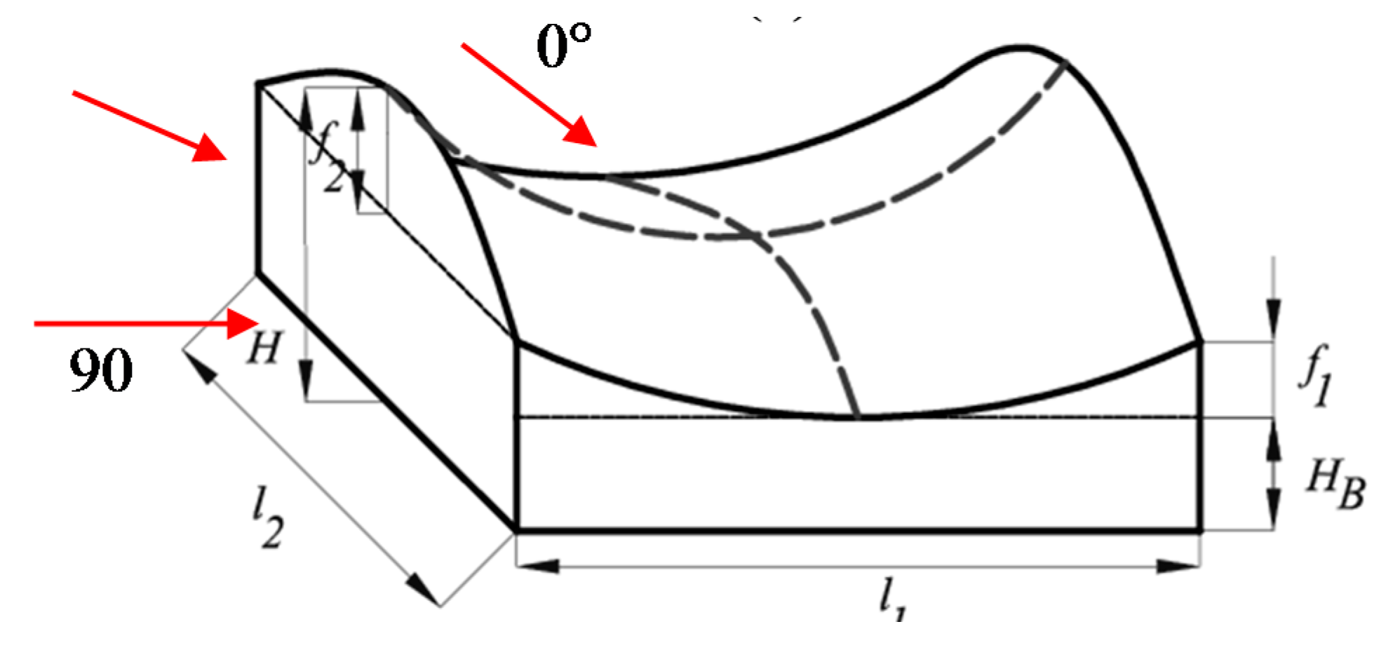
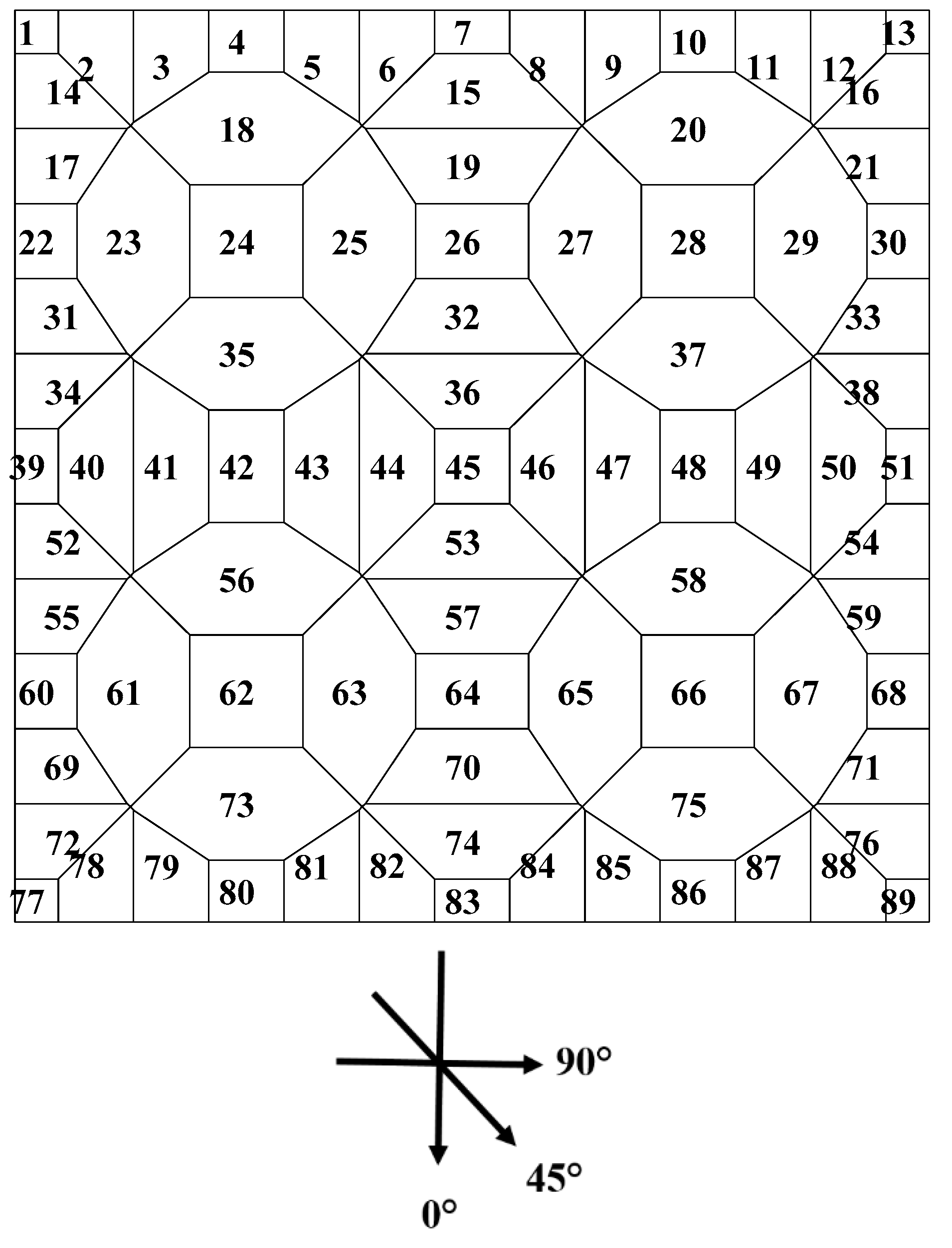
2. Geometrical Sample and Experimental Setup

Wind tunnel tests were carried out by [27] and [34] on 12 plan shapes, 2 different heights, and 2 different curvatures of buildings covered with hyperbolic paraboloid roofs.
This paper is focused on four of these samples and, in particular, on buildings that have a square plan, two different curvatures, and two different heights, described in [27,34,46], respectively.
Figure 1 shows the geometrical parameters listed in Table 1 for the geometries investigated. Parameters l1, f1, l2, and f2 are the upward and downward parabolas’ sags and spans, respectively. For the square plan, l1 is equal to l2; H is the sum of f1 + f2 and in this research, it was equal to 1/10 l1 (for model 1 and 2) and 1/6 l1 (for model 3 and 4 of l1 [27]); and HB is the distance between the ground and the lower point of the roof.
Aerodynamic tests were carried out in the open circuit CRIACIV (Interuniversity Research Center on Building Aerodynamics and Wind Engineering, city, country) wind tunnel with a developed boundary layer. The CRIACIV test chamber sizes are 2.4 × 1.6 m. The pressure series were acquired at a frequency equal to approximately 252 Hz for about 30 s [27,35]. The scaled models were made in wood and 1.5 mm Teflon diameter tubes instrumented the pressure taps. The pressure tap distribution on the square plan roofs is illustrated in Figure 2, which shows the Thiessen polygon shape for each pressure tap. In total, 89 pressure taps were located on the roof and 16 wind angles were acquired. The mean wind speed profile measured before placement of the model and its logarithmic approximation were estimated with z0 = 0.247 cm, model scale. This value was calculated by fitting the experimental points in the range of heights of interest, that is, from the ground level to the highest point of the roof. In a geometric scale of 1:100, this corresponds to a roughness length of 0.247 m, which is slightly lower than that of exposure category III of EN-1991 (z0 = 0.3 m), described as “area with regular cover of vegetation or buildings or with isolated obstacles with separations of maximum 20 obstacle heights (such as villages, suburban terrain, permanent forest)”.
The turbulence intensity profile at the roof level, ranges between 11% and 12%. The tests were performed at a mean wind speed of 16.7 m/s at a height of 10 cm, which, in a 1:100 scale, would be the standard reference height. Assuming that the prototype mean wind speed at 10 m of height is U = 27 m/s (design value for most of the Italian territory), then there is a velocity scale λv = 0.62, which corresponds to a time scale λt = 0.0162. Therefore, the 30 s model scale acquisition time corresponds to a full scale time of approximately 1800 s, well located within the interval of 600 s to 3600 s. The Reynolds number at model scale is about 9.4 × 10⁵, and 1.7 × 10⁸ at real scale. Turbulence intensity is about 10%. It is known that the Reynolds scale effect can affect results. However, it is expected that no Reynolds effects take place, because of the sharpness of the roof edges [33]. The longitudinal integral length scale at the roof height is about 30 cm at model scale, which would bring a full scale value lower than actual ones. This mismatch, common in most wind tunnel tests, is assumed to have minimal consequences on the results.
For the sake of brevity, the paper discusses only 0°, 45°, and 90° wind angles. More details about wind velocity, turbulence in wind tunnel, and wind tunnel setup were given in the work of [27].
The pressure coefficient c p was estimated according to Equation (1).
c p ( P , t ) = p ( P , t ) p 0 1 2 ρ V m 2
where p ( P , t ) is the measured pressure at point P of the roof surface, p 0 is the static pressure in the bare tunnel, and ½ r V2 m is the dynamic pressure measured by pressure taps.
Figure 3 shows an example of pressure coefficient time history (i.e., model 1, pressure tap #50, wind angle 0°); its maximum, minimum, mean, and mode values are overlapped on the time history. Figure 3 shows that the difference between mean and mode values is relevant for the pressure tap acquisition, taken as an example. However, the following results show that this trend is generalizable.
The pressure tap distribution chosen by the researchers closely affected the results. In fact, the processes acquired near the borders of the roof were statistically very different from others located in the middle of the roof [35].

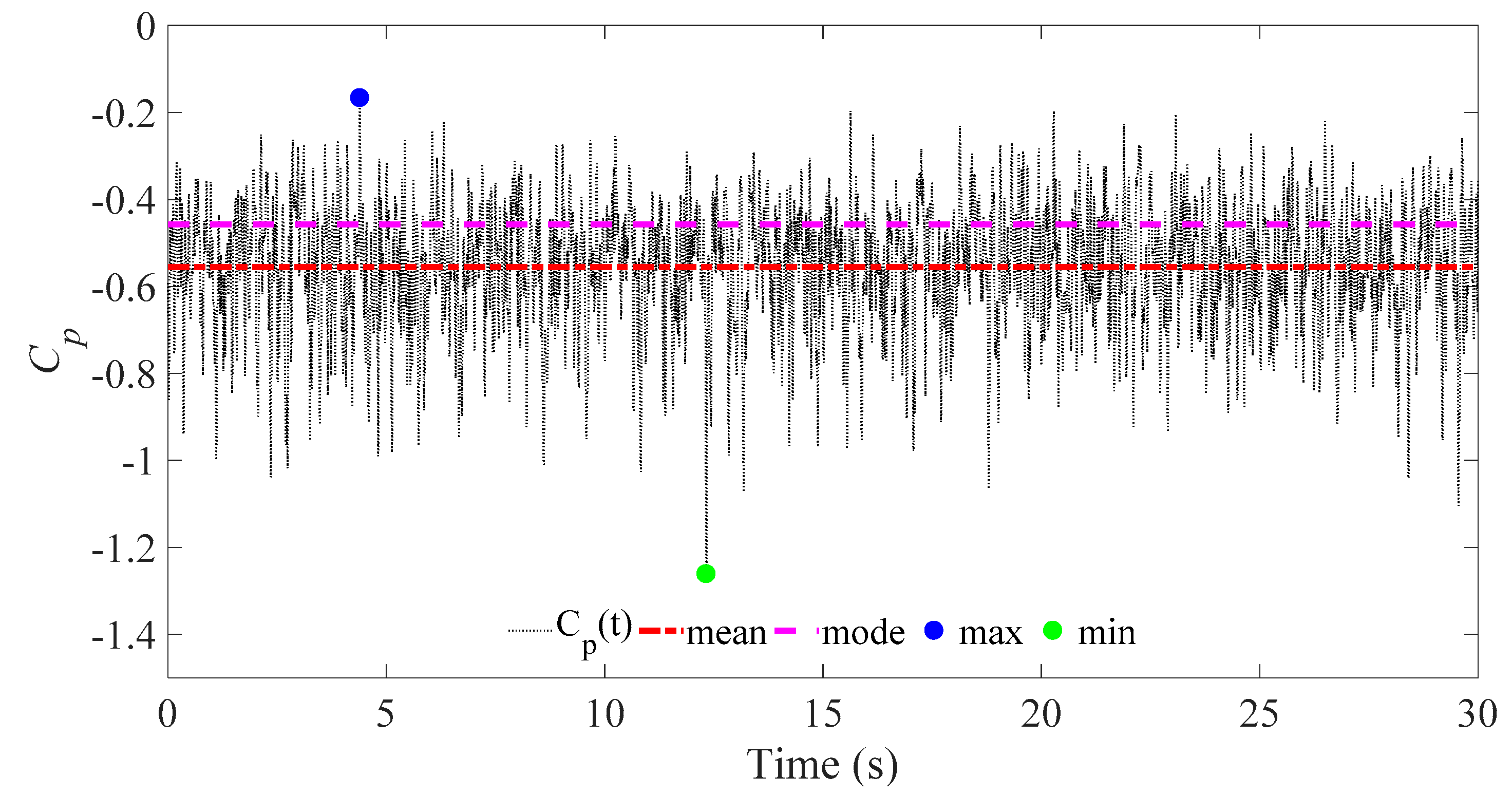
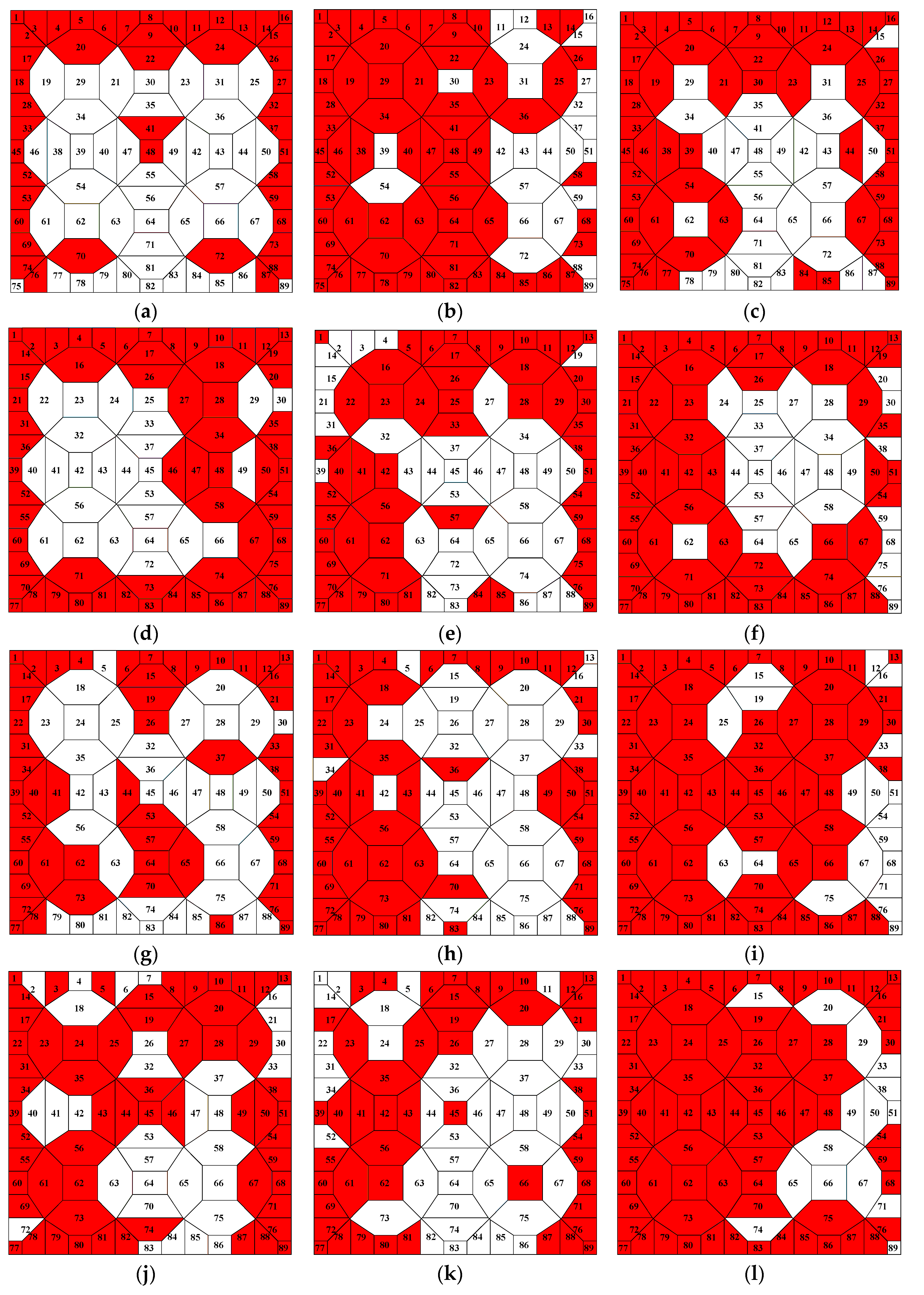
3. Experimental Data

Pressure coefficient time histories (i.e., in the following processes) were evaluated from pressure series acquired in wind tunnels. The statistical analyses of the pressure coefficient processes showed that some processes were Gaussian and others were non-Gaussian. The difference is crucial. As it is known, Gaussian processes are represented by mean and standard deviation, while for non-Gaussian processes, the mean value does not represent the process. Figure 4 shows the pdf (i.e., probability density function) of two examples of Gaussian (i.e., Figure 4a) and non-Gaussian (i.e., Figure 4b) processes. The two processes are estimated from series acquired on the same roof (i.e., model 1).
Figure 4a shows that mode is equal to the mean value, while on the contrary, Figure 4b shows that mode and mean are very different, with a ratio equal to 1.21. This trend suggests that the mean pressure coefficient maps may not adequately represent all processes on the roof. Similarly, the maxima and minima value maps are not representative because the extreme values are not simultaneous for all pressure taps.
It would desirable to put the pressure taps near borders because the vortex shedding caused by the 103 corners and the borders closely affected the pressure coefficient values
In order to investigate the Gaussian and non-Gaussian process distributions on the geometrical sample considered, Figure 5 represents the pressure taps that have non-Gaussian processes in red. This Gaussian characteristic was investigated both using the one-sided Kolmogorov–Smirnov test on the cdf (i.e., cumulative density function) of the processes compared with the normal cdf distribution, and following the work of [53]. According to the authors of [53], if the trend is Gaussian, the skewness γ3 and the excess kurtosis γ4 (i.e., kurtosis-3) should be less than or equal to 0.5.
Figure 5 shows the Gaussian (i.e., in white) and non-Gaussian (i.e., in red) processes for 0°, 45°, and 90° wind angles and for models 1 to 4.
Table 2 gives the percentage of Gaussian processes for all geometries and wind angles discussed in this paper.
For the geometry investigated (i.e., buildings covered with hyperbolic paraboloid roofs), the results show that the Gaussian process is closely affected by the building height, the curvature, and the wind angles.
On comparing different curvatures (i.e., model 1 and 2 with model 3 and 4), the results showed that for α = 0° (i.e., Figure 5a,d,g,j), the values were more affected by height and wind angles than by curvature. In fact, the number of Gaussian processes were similar between model 1 and 3 (i.e., the same height, but different curvature) and between model 2 and 4. The difference increased for α = 45° (i.e., Figure 5b,e,h,k) and α = 90° (Figure 5c,f,i,l). The number of Gaussian processes decreased when the height increased and when the radius of the curvature decreased (i.e., from model 1 and 2 surface to model 3 and 4 surface).
Globally, the wind angles closely affected the number of Gaussian processes. α = 90° had the smallest number of Gaussian processes (Figure 5c,f,i,l) and all values were smaller than 50%.
Considering the results shown in Figure 5, the mean pressure coefficient maps do not seem to be representative of most of the processes acquired. In Figure 5, white means Gaussian process and red means non-Gaussian process.
On this basis, the ratio between the mean value and the mode value, μ c p v c p , was calculated in order to measure the difference between them.
Figure 6 shows the μ c p v c p for each pressure tap and all the geometries and wind angles considered. In Figure 6, yellow means μ c p v c p > 1 ; purple means μ c p v c p < 1 ; and finally, white means μ c p v c p = 1 . Table 3 synthetizes the results. In particular, Table 3 gives the mean of μ c p v c p for all models (i.e., 1 to 4) and wind angles (i.e., α = 0°, 45°, and 90°), the percentage of μ c p v c p < 1 and μ c p v c p > 1 , and the mean of μ c p v c p for both (in brackets).
For α = 0° (Figure 6a,d,g,j), model 1 has 30.3% of processes for which the mean pressure coefficients underestimate the mode on average by 2%–3%. The percentage increases from model 2 to 4, with the maximum values equal to 56.2% for model 4.
For α = 45° (Figure 6b,e,h,k), model 1 has 41.6% of processes for which the mean pressure coefficients are lower than the mode on average by 2%–3%. The percentage increases in model 2, with maximum values equal to 46.1%. However, the percentage of processes with μ c p v c p < 1 is quite constant for all models, except for model 3, which has the smallest percentage, equal to about 28%.
For α = 90°, (Figure 6c,f,i,l), the percentage of μ c p v c p < 1 varies from 28.1% (i.e., model 2) to 38.2% (i.e., model 3 and 4). However, the mean of μ c p v c p , for μ c p v c p < 1 , increases from 2% to 3% for α = 0° and 45° from 5% to 8% for α = 90°.
The percentage of μ c p v c p > 1 is between 43.8% (i.e., model 4, α = 0°) and 71.9% (i.e., model 3, α = 45°).
The mean of μ c p v c p , for μ c p v c p > 1 , ranges from 1.03 (i.e., model 4, α = 0°) to 1.10 (i.e., model 1, α = 90°).
Regarding wind action estimation, if designers previously used mean pressure coefficients maps to design structures, the most dangerous situation was μ c p v c p < 1 , because the most frequent values of pressure coefficients did not correspond to the mean values used for its design. This means that the roof may be loaded differently. In order to take into account this aspect, using both the mean and mode pressure coefficient maps is suggested. These last maps, for Gaussian processes, correspond to mean pressure coefficient maps, while for non-Gaussian processes, the designer can choose the biggest value between mean and mode. This approach increases the reliability of the calculations.
Figure 7, Figure 8, Figure 9 and Figure 10 show a comparison between the mean pressure coefficient maps given by the authors of [27] (i.e., Figure 7a,c,e; Figure 8a,c,e; Figure 9a,c,e; and Figure 10a,c,e) and the mode pressure coefficient maps (i.e., Figure 7b,d,f; Figure 8b,d,f; Figure 9b,d,f; and Figure 10b,d,f).
Figure 7, Figure 8, Figure 9 and Figure 10 show that the trend is the same and that values vary slightly but, in many cases, significantly in term (i.e., 0–5%). However, as was previously discussed, this difference cannot be neglected for wind action on big surfaces varying up to 5% of wind loads.
It is reasonable to think that the wind load increase of 5% is negligible. This is true for many kinds of structures for which the dead and permanent loads are better than wind action (i.e., concrete, steel trusses, etc.). This cannot be true for flexible cables structures. It is important to specify that this value was obtained for this particular experiment’s campaign and shape. However, the paper aims to suggest an approach that is not taken into account, and the purpose is to suggest using both maps. The reason is that these structures are generally designed using equivalent static wind loads. When the shape is powered by codes, the static loads are generally estimated by equations that take into account mean values for the serviceability limit state, or maxima and minima for the ultimate limit state. Anyway, commonly, the Gaussianity is not discussed and so the representative role of the mean is not discussed either. In addition, the hyperbolic paraboloid net has two orders of cables—the first is upward and is load bearing for gravitational loads, while the second is downward and is load bearing for suction loads. If the sags of these two orders of cables are not equal (as is in the case of study investigated), the cables areas are different. This means that cables work differently under wind or under gravitational loads. Finally, in order to have a measure of this, take a practical example. Pressure taps are generally representative of roof areas. Each pressure tap, depending on the geometrical scale, corresponds to a specific zone in which the pressure coefficient is considered constant (i.e., experimental approximation due to the scaled model). In the case of study considered, each pressure tap represents at least 1/89 of the roof surface. If the geometrical scale of prototype is 1/100, it represents at least 72 m2 of the roof (about 8.5 m × 8.5 m). Considering a pressure in suction equal to 0.45 kN/m2 (0.5 × 1.25 × 272), and considering pressure coefficients equal to 1.5, cables are loaded by wind with forces equal to about 49 kN. Finally, considering that the dead and permanent loads are about 0.2 kN/m2, in the pressure tap area, there is a gravitational force equal to at least 14 kN (i.e., 0.9 kN for each node). The gravitational force is about 1/3 of the wind action. In this case, it corresponds to a uniformly distributed load on cables with a spacing equal to 2 m equal to (49 kN − 14 kN)/2 m = 17.5 kN/m or (49 kN × 1.05 − 14 kN)/2 m = 18.7 kN/m [27]. The difference is bigger than 7%. The cables traction load supports structures that are generally made of steel. It is important to consider that for steel structures, safety coefficients for material (i.e., material factors) given by Eurocode for the ultimate limit state are between 1 and 1.33. In particular, the safety coefficient for yielding of a metal face, shear failure of a profiled face, and support reaction capacity of a profiled face is equal to 1.1 (i.e., 10%). This value is dangerously close to 7%.

4. Conclusions

Experimental wind tunnel tests on roofs usually give pressure coefficient maps of mean, maxima, and minima values of the pressure series acquired. However, the measured processes are not all Gaussian along the entire roof, and most of these are considerably non-Gaussian. For these, the mean values are not as significant as the mode. This paper compares the mode and mean values of pressure coefficient time histories acquired in a wind tunnel on hyperbolic paraboloid roofs with square plans. In total, four different geometries were investigated, varying the building height and the hyperbolic paraboloid surface curvature. Three wind angles were taken into account, namely, 0°, 45°, and 90°. Mode pressure coefficients are given for all geometries and wind angles investigated.
The results showed that less than 50% of the processes were Gaussian and that the difference between the mean and mode values is up to 5%. Moreover, for 50% of the non-Gaussian processes, the mean is lower than the mode value. Regarding the investigated geometry (i.e., hyperbolic paraboloid roofs), the percentage of non-Gaussian processes was closely affected by height and mostly by wind angles.
Using both mean and mode pressure coefficient maps is suggested. These last maps, for Gaussian processes, correspond to mean pressure coefficient maps, while for non-Gaussian processes, the designer can choose the biggest value between mean and mode. This approach increases the reliability of the calculations.

Funding

This research received no external funding.

Conflicts of Interest

The author declares no conflict of interest.

References

  1. Lewis, W.J. Tension Structures: Form and Behavior; Thomas Telford: London, UK, 2003. [Google Scholar]
  2. Majowiecki, M. Tensostrutture: Progetto e Verifica; Edizioni Crea: Massa, Italy, 1994. [Google Scholar]
  3. Rizzo, F.; Zazzini, P. Improving the acoustical properties of an elliptical plan space with a cable net membrane roof. J. Acoust. Aust. 2016, 44, 449–456. [Google Scholar] [CrossRef]
  4. Rizzo, F.; Zazzini, P. Shape dependence of acoustic performances in buildings with a Hyperbolic Paraboloid cable net membrane roof. J. Acoust. Aust. 2017, 45, 421–443. [Google Scholar] [CrossRef]
  5. AIJ (Architectural Institute of Japan). Recommendations for Loads on Buildings; AIJ: Tokyo, Japan, 2004; Chapter 6: Wind Loads. [Google Scholar]
  6. ASCE (American Society of Civil Engineering). Wind Tunnel Studies of Buildings and Structures; Manuals of Practice (MOP); Isyumov, N., Ed.; ASCE: Reston, VA, USA, 1999; Volume 67. [Google Scholar]
  7. ASCE (American Society of Civil Engineering). Minimum Design Loads for Buildings and Other Structures; ASCE: Reston, VA, USA, 2010; Volume 7. [Google Scholar]
  8. AS/NZS (Standards Australia/Standards New Zealand). Structural Design Actions; Part 2: Wind Actions; AS/NZS 1170.2:2002; AS/NZS: Sydney, Australia, 2011. [Google Scholar]
  9. CEN (Comité Européen de Normalization). Eurocode 1: Actions on Structures—Part 1–4: General actions—Wind Actions; EN-1991-1-4; CEN: European Union, 2005. [Google Scholar]
  10. CNR (National Research Council of Italy). Guide for the Assessment of Wind Actions and Effects on Structures; CNR-DT 207/2008; CNR: Rome, Italy, 2008. [Google Scholar]
  11. Krishna, P.; Kumar, K.; Bhandari, N.M. Wind Loads on Buildings and Structures; Indian Standard IS:875, Part 3, Proposed Draft & Commentary; Wiley: New York, NY, USA, 2012. [Google Scholar]
  12. ISO (International Standards Organization). Wind Action on Structures—D.3 Wind Tunnel Testing Procedures; 4354:2012(E); ISO: Geneva, Switzerland, 2012. [Google Scholar]
  13. NRC/CNRC (National Research Council/Conseil National de Recherches Canada). Commentary to the National Building Code of Canada, Commentary I: Wind Load and Effects; NRC/CNRC: Ottawa, ON, Canada, 2010. [Google Scholar]
  14. SIA (Swiss Society of Engineers and Architects). Action on Structures—Appendix C: Force and Pressure Factors for Wind; SIA 261:2003; SIA: Zurich, Switzerland, 2003. [Google Scholar]
  15. Biagini, P.; Borri, C.; Facchini, L. Wind response of large roofs of stadiums and arena. J. Wind Eng. Ind. Aerodyn. 2007, 95, 9–11. [Google Scholar] [CrossRef]
  16. Dong, X.; Ye, J.H. Development and verification of a flow model of conical vortices on saddle roofs. J. Eng. Mech. 2015, 141, 04014127. [Google Scholar] [CrossRef]
  17. Elashkar, I.; Novak, M. Wind tunnel studies of cable roofs. J. Wind Eng. Ind. Aerodyn. 1983, 13, 407–419. [Google Scholar] [CrossRef]
  18. Kawai, H.; Yoshie, R. Wind-induced response of a large cantilevered roof. J. Wind Eng. Ind. Aerodyn. 1999, 83, 263–275. [Google Scholar] [CrossRef]
  19. Kawakita, S.; Bienkiewicz, B.; Cermak, J.E. Aeroelastic Model Study of Suspended Cable Roof; Fluid Mechanics and Wind Engineering Program, Department of Civil Engineering, Colorado State University: Fort Collins, CO, USA, 1992. [Google Scholar]
  20. Killen, G.P.; Letchford, C.W. A parametric study of wind loads on grandstand roofs. Eng. Struct. 2001, 23, 725–735. [Google Scholar] [CrossRef]
  21. Kimoto, E.; Kawamura, S. Aerodynamic criteria of hanging roofs for structural Design. In Proceedings of the IASS Symposium on Membrane Structures and Space Frames, Osaka, Japan, 15–19 September 1986. [Google Scholar]
  22. Irwin, H.P.A.H.; Wardlaw, R.L.A. Wind tunnel investigation of a retractable fabric roof for the Montreal Olympic stadium. In Proceedings of the 5th International Conference on Wind Engineering, Fort Collins, CO, USA, 8–14 July 1979; pp. 925–938. [Google Scholar]
  23. Letchford, C.W.; Killen, G.P. Equivalent static wind loads for cantilevered grandstand roofs. Eng. Struct. 2002, 24, 207–217. [Google Scholar] [CrossRef]
  24. Vitale, A.; Letchford, C.W. Full-scale wind loads on a porous canopy roof. In Proceedings of the Australasian Structural Engineering Conference, Auckland, New Zealand, 30 September–2 October 1998. [Google Scholar]
  25. Letchford, C.W.; Denoon, R.O.; Johnson, G.; Mallam, A. Dynamic characteristics of cantilever grandstand roofs. Eng. Struct. 2002, 24, 1085–1090. [Google Scholar] [CrossRef]
  26. Rizzo, F.; Sepe, V.; Vasta, V. Correlation structure of wind-tunnel pressure fields for a hyperbolic paraboloid roof. In Proceedings of the Italian Association of Theoretical and Applied Mechanics (AIMETA 2017), Salerno, Italy, 4–7 September 2017; Gechi Edizioni: Salerno, Italy, 2017; ISBN 978-889-42484-7-0. [Google Scholar]
  27. Rizzo, F. Wind tunnel tests on hyperbolic paraboloid roofs with elliptical plane shapes. Eng. Struct. 2012, 45, 536–558. [Google Scholar] [CrossRef]
  28. Rizzo, F.; D’Asdia, P.; Lazzari, M.; Procino, L. Wind action evaluation on tension roofs of hyperbolic paraboloid shape. Eng. Struct. 2011, 33, 445–461. [Google Scholar] [CrossRef] [Green Version]
  29. Rizzo, F.; D’Asdia, P.; Procino, L.; Lazzari, M.; Olivato, G. Aerodynamic behavior of hyperbolic parabolic shaped roofs: Wind tunnel test, POD and CFD analysis. In Proceedings of the 12th International Conference on Civil, Structural and Environmental Engineering Computing (CC 2009), Madeira, Portugal, 1–4 September 2009. [Google Scholar]
  30. Rizzo, F.; D’Asdia, P.; Lazzari, M.; Olivato, G. Aerodynamic behavior of hyperbolic paraboloid shaped roofs: POD and CFD analysis. In Proceedings of the 5th European & African Conference on Wind Engineering (EACWE 5 2009), Florence, Italy, 19–23 July 2009. [Google Scholar]
  31. Rizzo, F.; D’Asdia, P.; Lazzari, M. Aerodynamic behavior of hyperbolic paraboloid shaped roofs: Wind tunnel tests. In Proceedings of the 5th European & African Conference on Wind Engineering (EACWE 5 2009), Florence, Italy, 19–23 July 2009. [Google Scholar]
  32. Sykes, D.M. Wind loading tests on models of two tension structures for EXPO’92, Seville. J. Wind Eng. Ind. Aerodyn. 1994, 52, 371–383. [Google Scholar] [CrossRef]
  33. Sun, X.; Wu, Y.; Yang, Q.; Shen, S. Wind tunnel tests on the aeroelastic behaviors of tension structures. In Proceedings of the VI International Colloquium on Bluff Bodies Aerodynamics & Applications, BBAA VI, Milan, Italy, 20–24 July 2008. [Google Scholar]
  34. Rizzo, F.; Ricciardelli, F. Design pressure coefficients for circular and elliptical plan structures with hyperbolic paraboloid roof. J. Eng. Struct. 2017, 139, 153–169. [Google Scholar] [CrossRef]
  35. Rizzo, F.; D’Asdia, P.; Ricciardelli, F.; Bartoli, G. Characterization of pressure coefficients on hyperbolic paraboloid roofs. J. Wind Eng. Ind. Aerodyn. 2012, 102, 61–71. [Google Scholar] [CrossRef]
  36. Rizzo, F.; Barbato, M.; Sepe, V. Peak factor statistics of wind effects for hyperbolic paraboloid roofs. Eng. Struct. 2018, 173, 313–330. [Google Scholar] [CrossRef]
  37. Liu, M.; Chen, X.; Yang, Q. Characteristics of dynamic pressures on a saddle type roof in various boundary layer flows. J. Wind Eng. Ind. Aerodyn. 2016, 150, 1–14. [Google Scholar] [CrossRef]
  38. Brito, R.; Caracoglia, L. Extraction of flutter derivatives from small scale wind tunnel experiments. In Proceedings of the 11th Americas Conference on Wind Engineering, American Association for Wind Engineering (AAWE), San Juan, Puerto Rico, 22–26 June 2009. [Google Scholar]
  39. Rizzo, F.; Caracoglia, L.; Montelpare, S. Predicting the flutter speed of a pedestrian suspension bridge through examination of laboratory experimental errors. Eng. Struct. 2018, 172, 589–613. [Google Scholar] [CrossRef]
  40. Rizzo, F.; Caracoglia, L. Examining wind tunnel errors in Scanlan derivatives and flutter speed of a closed-box. J. Wind Struct. 2018, 26, 231–251. [Google Scholar]
  41. Avossa, A.M.; Di Giacinto, D.; Malangone, P.; Rizzo, F. Seismic Retrofit of a Multi-Span Prestressed Concrete Girder Bridge with Friction Pendulum Devices. Shock Vib. 2018. [Google Scholar] [CrossRef]
  42. Daw, D.J.; Davenport, A.G. Aerodynamic damping and stiffness of a semi-circular roof in turbulent wind. J. Wind Eng. Ind. Aerodyn. 1989, 32, 83–92. [Google Scholar] [CrossRef]
  43. Forster, B. Cable and membrane roofs, a historical survey. Struct. Eng. Rev. 1994, 6, 3–5. [Google Scholar]
  44. Kassem, M.; Novak, M. Wind-Induced response of hemispherical air-supported Structures. J. Wind Eng. Ind. Aerodyn. 1992, 41, 177–178. [Google Scholar] [CrossRef]
  45. Knudson, W.C. Recent advances in the field of long span tension structures. Eng. Struct. 1991, 13, 174–193. [Google Scholar] [CrossRef]
  46. Pun, P.K.F.; Letchford, C.W. Analysis of a tension membrane HYPAR roof subjected to fluctuating wind loads. In Proceedings of the 3rd Asia-Pacific Symposium on Wind Engineering, Hong Kong, 13–15 December 1993; pp. 741–746. [Google Scholar]
  47. Rizzo, F.; Sepe, V. Static loads to simulate dynamic effects of wind on hyperbolic paraboloid roofs with square plan. J. Wind Eng. Ind. Aerodyn. 2015, 137, 46–57. [Google Scholar] [CrossRef]
  48. Shen, S.; Yang, Q. Wind-induced response analysis and wind-resistant design of hyperbolic paraboloid cable net structures. Int. J. Space Struct. 1999, 14, 57–65. [Google Scholar] [CrossRef]
  49. Vassilopoulou, I.; Gantes, C.J. Nonlinear dynamic behavior of saddle form cable nets under uniform harmonic load. Eng. Struct. 2011, 33, 2762–2771. [Google Scholar] [CrossRef]
  50. Vassilopoulou, I.; Gantes, C.J. Vibration modes and natural frequencies of saddle form cable nets. Comput. Struct. 2012, 88, 105–119. [Google Scholar] [CrossRef]
  51. Vassilopoulou, I.; Petrini, F.; Gantes, C.J. Nonlinear dynamic behavior of cable nets subjected to wind loading. Structures 2017, 10, 170–183. [Google Scholar] [CrossRef]
  52. Yang, Q.; Liu, R. On Aerodynamic Stability of Membrane Structures. Int. J. Space Struct. 2005, 20, 181–188. [Google Scholar] [CrossRef]
  53. Suresh Kumar, K.; Stathopoulos, T. Wind loads on low building roofs: A stochastic perspective. J. Struct. Eng. 2000, 126, 944–956. [Google Scholar] [CrossRef]
Figure 1. Geometrical parameters.
Computation 06 00064 g001
Figure 2. Thiessen polygons distribution.
Computation 06 00064 g002
Figure 3. Examples of pressure coefficients time history: model 1, pressure tap #50, wind angle 0°.
Computation 06 00064 g003
Figure 4. Gaussian process, model 1, #19 = 0° pdf (probability density function) (a); non-Gaussian process #2 = 0° (b).
Computation 06 00064 g004
Figure 5. Gaussian process distribution on the roofs, model 1 α = 0° (a), α = 45° (b), and α = 90° (c); model 2 α = 0° (d), α = 45° (e), and α = 90° (f); model 3 α = 0° (g), α = 45° (h), and α = 90° (i); model 4 α = 0° (j), α = 45° (k), and α = 90° (l).
Computation 06 00064 g005
Figure 6. Ratio μ c p v c p distribution on the roofs, model 1 α = 0° (a), α = 45° (b), and α = 90° (c); model 2 α = 0° (d), α = 45° (e), and α = 90° (f); model 3 α = 0° (g), α = 45° (h), and α = 90° (i); model 4 α = 0° (j), α = 45° (k), and α = 90° (l).
Computation 06 00064 g006
Figure 7. Model 1, mean pressure coefficient maps for α = 0° (a), α = 45° (c), and α = 90° (e); maps using mode of pressure coefficients for α = 0° (b), α = 45° (d), and α = 90° (f).
Computation 06 00064 g007
Figure 8. Model 2, mean pressure coefficient maps for α = 0° (a), α = 45° (c), and α = 90° (e); maps using mode of pressure coefficients for α = 0° (b), α = 45° (d), and α = 90° (f).
Computation 06 00064 g008
Figure 9. Model 3, mean pressure coefficient maps for α = 0° (a), α = 45° (c), and α = 90° (e); maps using mode of pressure coefficients for α = 0° (b), α = 45° (d), and α = 90° (f).
Computation 06 00064 g009
Figure 10. Model 4, mean pressure coefficient maps for α = 0° (a), α = 45° (c), and α = 90° (e); maps using mode of pressure coefficients for α = 0° (b), α = 45° (d), and α = 90° (f).
Computation 06 00064 g010
Table 1. Wind tunnel model sizes.
Modell1 [cm]l2 [cm]f1 [cm]f2 [cm]H [cm]HB [cm]
180.0080.002.675.338.0013.33
280.0080.002.675.338.0026.66
380.0080.004.448.8913.3313.33
480.0080.004.448.8913.3326.66
Table 2. Percentage of Gaussian processes.
Modelα = 0°α = 45°α = 90°
144.927.032.6
229.240.428.1
341.641.621.3
434.846.116.9
Table 3. Mean value of μ c p v c p and percentage of cases where μ c p v c p < 1 and μ c p v c p > 1 .
Modelα = 0°α = 45°α = 90°
Mean of ( μ c p v c p ) ratio
11.031.011.05
21.031.011.05
31.021.021.01
41.001.011.02
Percentage of cases where
( μ c p v c p ) < 1 (%)
Value in parenthesis is the mean value of the ratio restricted to cases where ratio <1
130.341.632.6
(0.98)(0.97)(0.94)
236.046.128.1
(0.99)(0.98)(0.95)
334.828.138.2
(0.98)(0.97)(0.87)
456.241.638.2
(0.97)(0.98)(0.92)
Percentage of cases where
( μ c p v c p ) > 1 (%)
Value in parenthesis is the mean value of the ratio restricted to cases where ratio >1
169.758.467.4
(1.05)(1.04)(1.10)
264.053.971.9
(1.05)(1.03)(1.09)
365.271.961.8
(1.04)(1.04)(1.10)
443.858.461.8
(1.03)(1.03)(1.08)

