Advanced Markov-Based Machine Learning Framework for Making Adaptive Trading System


1
STMicroelectronics ADG—Central R&D, 95121 Catania, Italy
2
IPLAB—Department of Mathematics and Computer Science, University of Catania, 95121 Catania, Italy
3
GIURIMATICA Lab, Department of Applied Mathematics and LawTech; 97100 Ragusa, Italy
*
Author to whom correspondence should be addressed.
Computation 2019, 7(1), 4; https://0-doi-org.brum.beds.ac.uk/10.3390/computation7010004
Submission received: 14 November 2018
/
Revised: 19 December 2018
/
Accepted: 28 December 2018
/
Published: 3 January 2019
(This article belongs to the Section Computational Engineering)
Abstract
:Stock market prediction and trading has attracted the effort of many researchers in several scientific areas because it is a challenging task due to the high complexity of the market. More investors put their effort to the development of a systematic approach, i.e., the so called “Trading System (TS)” for stocks pricing and trend prediction. The introduction of the Trading On-Line (TOL) has significantly improved the overall number of daily transactions on the stock market with the consequent increasing of the market complexity and liquidity. One of the most main consequence of the TOL is the “automatic trading”, i.e., an ad-hoc algorithmic robot able to automatically analyze a lot of financial data with target to open/close several trading operations in such reduced time for increasing the profitability of the trading system. When the number of such automatic operations increase significantly, the trading approach is known as High Frequency Trading (HFT). In this context, recently, the usage of machine learning has improved the robustness of the trading systems including HFT sector. The authors propose an innovative approach based on usage of ad-hoc machine learning approach, starting from historical data analysis, is able to perform careful stock price prediction. The stock price prediction accuracy is further improved by using adaptive correction based on the hypothesis that stock price formation is regulated by Markov stochastic propriety. The validation results applied to such shares and financial instruments confirms the robustness and effectiveness of the proposed automatic trading algorithm.
1. Introduction
Stock price prediction is one of the main challenging tasks of the financial area. In literature, there are several algorithms showing approaches for stock price prediction. Initially, the research investigation focused its effort on methods based on traditional statistical algorithms, as well as on the usage of soft computing techniques [1]. The recalled classical approaches show their limitation related to inflexibility in dynamic variability and complexity. The major issue of stock price forecast is related to high unpredictability, especially for long term prediction. Perhaps a valuable impact on stock price variability is correlated to economic news or—for some stocks—to national and international government policy. Countless research studies showed that a good and robust financial market model for stock price forecast needs the development of algorithms able to process a lot of mathematical and econometric variables; especially in the short term prediction of stock price. Nonetheless, there is a huge amount of studies of various disciplines that have attempted to address the task of stock price prediction, presenting a large variety of approaches, even though it seems, from general comparative results, that soft computing and more recent machine learning approaches exceed classical algorithms in terms of performance. In the next sections, we describe some of the developed algorithms for stock price prediction starting from classical ones based on regressive models, until the recent ones based on Machine learning modelling.
1.1. Stock Price Prediction Methods Prior Art: Classical Pipelines
One of the first work about stock prediction is in Reference [2] where the authors presented a buying and selling timing prediction system for stocks by using modular neural networks. Wang et al. in Reference [3] presents a prediction system for stock market by utilizing a non-linear an Autoregressive Integrated Moving Average (ARIMA) model. The authors reached effective results in stock market prediction by using an Autocorrelation Function (ACF) to verify if a time series is stationary or non-stationary in order to remove non-stationary behavior. The authors implement an ARIMA-based recurrent network for stock market prediction. The experimental results confirmed that the proposed approach seems quite good even though the prediction accuracy can be improved by filtering stock price series in order to involve noise in it. In Reference [1], the authors propose a Genetic Algorithms (GA) approach in order to predict a stock price index. They basically focus on feature discretization in order to reduce the complexity in feature space. The approach consists of the combination of a generic algorithm and together with an Artificial Neural Networks (ANN) hybrid system in order to optimize the connection weights between layers and the thresholds for feature discretization. Despite presenting some limitations, the approach seems very promising. One limitation is that the performance of the model varies according to the number of the elements in the hidden layers. Additionally, the weights and the thresholds must be determined accurately to avoid the ANN overfitting problem. Another approach, based on neural networks, uses ANN [4]. The authors exploit ANN in order to select the most significant factors that affect the daily direction of S&P 500 index. The results are promising even if it is difficult to determine the optimal network parameters and select significant features. All the described methods suffer from a limited ability to financial timeseries generalization of the used mathematical models. Significant improvements in addressing the aforementioned issue occurred with the adoption of modern Machine Learning techniques, as described in the next section.
1.2. Stock Price Prediction Methods Prior Art: Recent Machine and Deep Learning Pipelines
In Reference [5], the authors try to implement a Long Short-Term Memory (LSTM) model to predict stock value movement. Specifically, Nelson et al. implement a LSTM classification model in order to determine if the price of a particular stock will be higher or not than the current price in 15 min in the future. The results show that the model based on LSTM is more accurate than other machine learning models. A very interesting approach is described in Reference [6]: Zhang et al. used, successfully, the Elman Recurrent Neural Network for predicting the open price of such stocks. Specifically, the author described the Particle Swarm Optimization (PSO) algorithm for learning optimization of the Elman Recurrent Neural Network. The experimental results confirmed that the proposed approaches seems very promising, even though the prediction benchmark seems comparable to classical BP Neural Network algorithms [6]. Another survey about usage of Machine Learning for stock market prediction is reported in Reference [7]. The authors provide a detailed benchmark about usage of Support Vector Machine (SVM), Random Forest, K-Nearest Neighbor (KNN), Naive Bayes, and Softmax in stock prediction. The experimental results confirmed that Random Forest algorithm performs the best for large datasets, and Naïve Bayesian Classifier is the best for small datasets. The results also reveal that reduction in the number of technical indicators reduces the accuracies of each algorithm. Anyway, from careful analysis of the recalled prior-art, the authors identified a common baseline of almost of the Machine Learning algorithms: All methods perform a stock price prediction by using historical data, and in some cases, data coming from sentiment analysis [8].
1.3. The Proposed Stock Price Prediction Systems: Brief Overview of Underlying Algorithm
The work herein described, goes in the direction drawn by the Machine Learning methods above detailed: We propose the usage of Long Short-Term Memory (LSTM) architecture [9] for performing an adaptive profitable trading system for stock markets. The adoption of LSTM is correlated to a specific study we have performed about financial time series dynamics. Starting from that statistic analysis, we introduce some specific hypothesis on price formation dynamic. Basically, we assume that the stock price formation is influenced by previous price timeserie, i.e., price forecast of such stocks is affected by the previous trend of the same stock. In this regard, the LSTM have gained a lot of credit because of their peculiarity, which allows time series forecasting starting from the previous values of the series. The LSTMs are perfectly suited to this task as they are able to learn from past collected information included in the stock price dynamic making a prediction based on that data. In this context, the authors proposed a LSTM based algorithms for the prediction of stock close price in a daily timeframe. Moreover, taking into account the above statistic hypothesis, the authors have developed a further improvement of the LSTM stock price and trend prediction based on specific assumption that share price formation satisfies the Markov statistical hypothesis. In order to show the robustness of the proposed approach, we have tested the algorithm analyzing high volatile shares such as bank stocks considering, perhaps, the current unstable macro-economic dynamics. We collected about 18 years of historic bank stocks daily close price time series from October 2000 to October 2018, downloaded from Yahoo-finance website, details follow.
The aim of this paper is to forecast “close price” of such stocks across a given timeframe in order to elaborate ad-hoc trading algorithm based on that prediction. The remainder of the paper is structured as follows. In Section 2 we introduce the forecasting problem and an overview of our strategy and a brief introduction about Long Short-Term Memory neural networks and their structure. We present, in Section 3 and Section 4, our proposed method and an introduction about referred Markov propriety. In Section 5, we show some experimental results about advantages and applications of our method. In Section 6, we present a short discussion about future work.
2. The Overall Framework
2.1. Stock Price Forecasting Problem
Stock price forecasting can be defined as the prediction of current share price by using historical data of same stock as well as correlated ones such market indexes, similar stocks, etc. Many regression models are designed for explanatory purposes to understand the correlation between relevant economic factors. Classical Regression models are often used for quantitative shares dynamic forecasting. The desired target is to accurately predict the “future”. A reliable forecasting algorithm will be able to identify risk factors, market indexes, and estimated rate of win/loss trades in investment decisions, as well as the impact of critical events such as default rates and so on [10,11]. Specifically, the forecast of financial time series allows to understand stock market trend as it plays a key role on making investment decisions. Moreover, the forecast financial times-series allows for the identification of specific patterns useful to predict the best performing corporate shares or market indexes. Those evaluations make time series analysis and forecasting an important area of research. In this work, we propose a forecasting algorithm for stock price and trend prediction as well as a correlated trading system based on those predictions. As recalled previously, a robust prediction system should be able to forecast the current market trend so that we have implemented two pipelines of LSTMs: One for global trend prediction and other for stock close price forecast.
2.2. Mathematical Background of LSTM
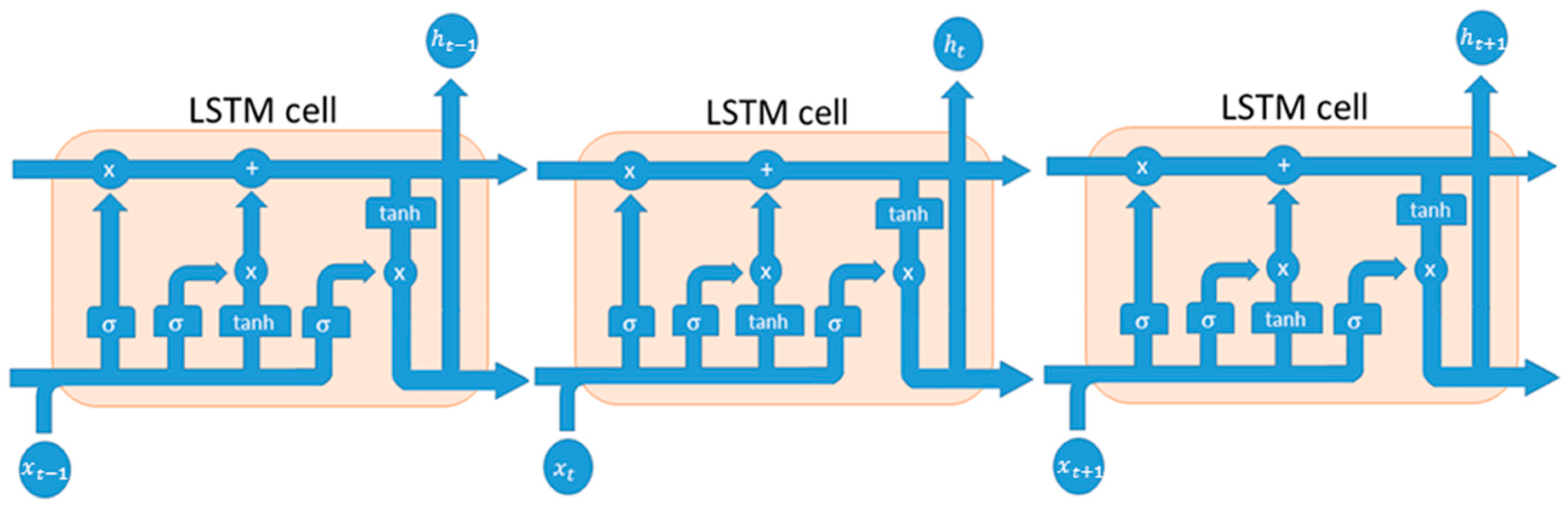
The LSTM is a particular type of Recurrent Neural Network (RNN) with effective performance in regression problem such as forecasting time series. LSTM mode description is carefully detailed in Reference [9]. LSTMs represent a considerable improvement of the classic RNN model because they are able to evaluate the hidden nonlinear correlations between and within input data that has led to increasing the performance of the time-series prediction algorithm. A classical LSTM main unit is composed of a cell and an input/output/forget gate. The cell is able to store (recall) values over arbitrary time intervals, while the above gates are able to manage the input/output data flow of the cell. The diagram of a typical structure of a LSTM cell as well as related equation model is reported in Figure 1.
More details is shown in Figure 2 I where a prototype of LSTM cell is shown.
Basically, the input of LSTM is a vector that represents the old memory and it passes through the forget layer that decides what information it can throw away from the cell state. According to this, the “forget gate layer” verifies the value of each number present in cell , where ‘1’ represents information to keep, while ‘0’ represents information to forget (1).
Then, we decide what new information we’re going to store in the cell state using Equations (2) and (3) in order to merge the new and the old memory, where is the value that can be added to the cell states and identifies the activation values of the input gates.
The next step updates the old cell state into the new cell state, called , as reported by Equation (4).
Finally, we generate the LSTM output by merging the previous output, the input and the bias vector according to the following Equations (5) and (6).
where:
- represent the LSTM weights
- are the bias
- is the cell state
- is the sigmoid function
Several research papers [12] confirmed that LSTM networks are well-suited for classifying, analyzing and—as in this case—making time series forecasting as their mathematical model was developed to deal with the exploding and vanishing gradient problems usually raised in the classical RNNs architecture. For instance, one of the most recent work about LSTM-CNN based system for classification is in Reference [13]. The authors present an interesting approach to improve classification task, in particular, their method consists in reducing the execution time by 30%–42%. Thus, they prove the effectiveness of LSTM neural network and their important contribution for specific tasks. Now, after LSTM model introduction, we are ready to describe the proposed forecasting algorithm and related trading system. Afterwards, we report several scenarios in which the proposed approach shows high predictability and profitability.
3. The LSTMs Forecasting Framework: Description
Our prediction framework is composed by two LSTM networks: One for trend prediction and another one for stock close price time-series regression. The first implemented LSTM network is used for stock trend forecast: it is basically composed of an input layer in which we fed one stock close price value at once; an hidden layer of 400 neurons and finally a fully connected output layer (one neuron). The second LSTMs layer shows the same structure, but some configuration parameters and training updates are different because it will be used for stock close price prediction. To validate the method, we decided to select historical data (Daily timeframe) about bank stocks (e.g., Unicredit [UCG.MI], Monte dei Paschi di Siena [MPS.MI], Intesa San Paolo [ISP.MI], and Credito Valtellinese [CVAL.MI], etc.), as well as a corporate share i.e., Enel [ENEL.MI], all listed in the Milano Stock Exchange Market. All daily data have been downloaded from Yahoo Finance website [14]. The historical data have been collected from October 2000 to October 2018 and each entry is referred to daily timeframe. Specifically, we collected for each share: Daily Open/Close/High/Low prices even though we validate our system only for Close prediction. All collected financial values have been arranged as part of training set and part as validation set. All values were normalized in the range (−1, 1), with classical MinMaxScaler algorithm. In Figure 3 we show an instance of the stock included in the arranged dataset (Unicredit) in which the blue-colored part of the share timeserie represents the data we collected as training set, while the remaining ones (red-colored) is used as a test and validation set of the proposed approach. In more detail, in order to perform a valid and robust training session, we considered about 12 years of the 18 collected that denotes about 2900 input data (highlighted by green rectangle), as per previous description. The remaining six years (about 1600 data) are used as the validation set of the proposed pipeline.
In Figure 4, the authors report an overall representation of the proposed pipeline (the part devoted to the stock trend and price prediction) in order to show the processing flow we have designed to reach the desired targets: An efficient stock price and trend prediction algorithm.
The proposed stock trend and price prediction pipeline is then composed by the following components: A data pre-processing block followed by the two pipeline LSTM framework (in which one pipeline for Trend prediction and another one for stock price prediction). The first block (data pre-processing) is able to normalize input stock price timeserie data, as well as to split input data between training and validation, as above described. The so processed data are fed into LSTM framework in which it will be properly processed in order to provide an estimation of the mid-long term trend (LSTM Trend direction prediction), as well as of the stock prices (LSTM Prediction from real data). About this latest block, the proposed stock close price prediction system is based on the usage of LSTM together with mathematical price correction approach based on the usage of the so-called Markov statistical model. We introduce now a brief overview of the Markov model theory needed to understand the proposed enhanced of the LSTM prediction system. As reported in Reference [15], the Markov Model based approaches for financial time-series forecasting shows promising results. In Reference [15], for instance, the authors described a predicting method based on usage of Hidden Markov Model in order to improve the accuracy and a comparison of the existing techniques based on Machine and Deep learning. As is well known, a stochastic process can be defined as “Markov Process” if the underlying dynamic satisfies the Markov propriety, i.e., the probability of an event—in a well defined sequence—depends only on the state attained in the previous event. Formerly, in the discrete-time domain, if we consider a random variable X with Markov propriety with a related probabilistic sequence , we have:
The financial research area confirmed the fundamental role of probability theory and stochastic analysis in the share price formation. As reported in Reference [15], in the context of stochastic analysis the Markov theory (Markov Chain, Hidden Markov Mode, Markov propriety, etc.) shows very promising results in addressing financial time series forecasting problem. More in detail, a very effective Markov based approach for addressing financial data processing issues is the assumption that price formation satisfies Markov propriety. Specifically applied in the proposed approach, the authors perform a further processing of that assumption: We assume that if the price value at specific time yt+1 depends of previous stock price value only yt, the related prediction error et+1 keeps same statistics, i.e., it satisfies Markov propriety so that the current stock price prediction error et+1 is correlated to previous ones et only. We have applied this assumption to our prediction model based on LSTMs, as described in what follows. Formerly, we consider stock close price prediction made by the second LSTM pipeline, as pointed out in Figure 4.
In Equation (9), we have indicated as the stock close price at previous time t – 1, while represents the second LSTM prediction functional model, and then, represents the forecasted stock close price. In our theory framework, we define Y as the random variable describing the stock price formation under the implicit hypothesis that stock price formation satisfies Markov propriety, i.e., under the following mathematical correlation:
According to Equation (10), we have similarly supposed that the error prediction dynamic satisfies the same Markov propriety. Formerly, if we consider E as the random variable describing the prediction error evolution, the same correlation reported in Equation (9) is satisfied:
Equation (11) means, in few words, that under the adopted hypothesis (stock price prediction error dynamic satisfies the Markov propriety) we have the great advantage to use the previous prediction error et to correct the current stock price forecasting process. Therefore, according to this clear consequence, we proceed correcting the stock close price prediction performed by our LSTM system as per Equation (9) with a part of previous stock close price prediction error, as reported below:
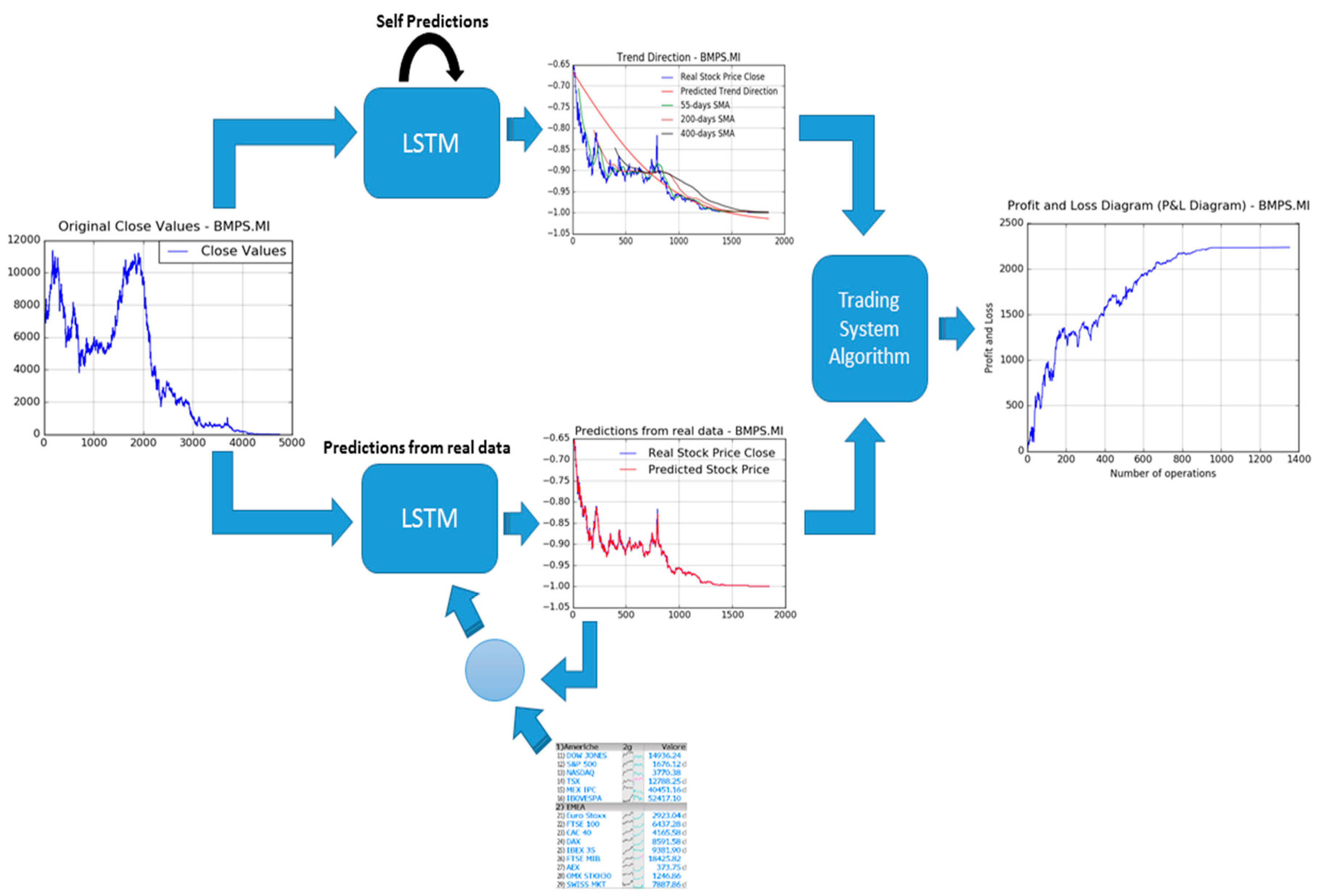
where, with the parameter p, we have defined a learning adaptive factor heuristically determined (we have configured p = 0.5 for this work), while we have defined as the real stock close price, and with , the predicted ones by second LSTM pipeline (see Equation (9)). Consequently, after an appropriate training session, this part of the proposed pipeline, will be used as stock close price forward predictor. Specifically, during market evolution we select a stock and then use collected actual stock close price value at time t for forecasting the same share close price at time t + 1. By means of the made assumption, that price formation satisfies Markov propriety, the so obtained prediction (made by the second LSTM) will be furtherly corrected by means of the previous prediction error, as per Equation (12). Meanwhile, the first LSTM pipeline performs mid-long term trend forecast. Considering that we collect stock market prices at real time (according to adopted timeframe) we have decide to improve LSTM predictability to update the second LSTM pipeline with already collected real stock close prices. In this way, we improve the prediction accuracy of the second LSTM pipeline because we update the internal representation of the stock timeserie (acquired during the training session) with real-time data being collected. Afterwards, considering that we have predicted the mid-long stock trend as well as the next stock close price, we are ready to decide what type of financial operation to be performed. For this reason, the so predicted stock prices (from second LSTM) as well as the predicted trend information (first LSTM) will be fed into the Trading System Algorithm block to make a decision about the trade to be done (LONG vs SHORT vs Null Operation) as well as to estimate related trade parameters such as Take Profit (pre-defined amount of profit for the related trade), Stop Loss (max accepted loss for the analyzed trade), and so on. In Figure 5, an overall scheme of the whole proposed financial pipeline is reported.
The pipeline described in Figure 5 is a clear graphical representation of the algorithm described till now, i.e., the two LSTM pipelines for mid-long term trend prediction (Self Predictions LSTM as the deep neural network performs mid-long term trend prediction by recurrent learning of stock price timeserie without update with real data being collected) and stock close price predictions (Predictions from real data as this second LSTM—as said above—will perform a real-time update of each internal representation by using real stock prices data being collected during market session) and the new block named “Trading System Algorithm” block, which will be better described in the next section.
4. The Trading System Algorithm Block
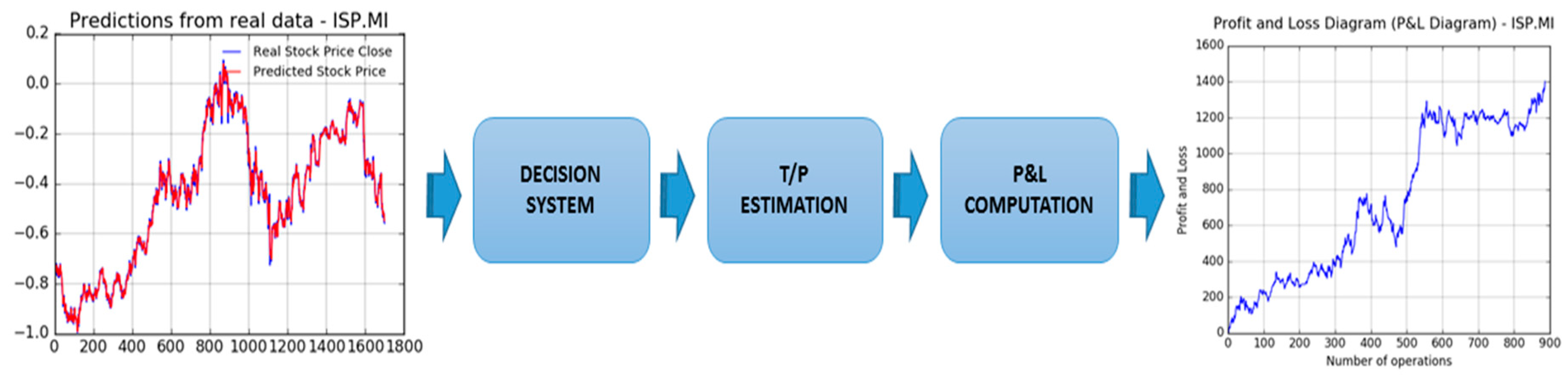
In this section, we describe the latest block of the proposed pipeline reported in Figure 5. In the following Figure 6, the functional pipeline embedded in the trading system block is shown.
The first target of this block is the analysis of the mid-long term trend prediction made by the first LSTM. This analysis based on mathematical check of the LSTM output (simple derivative analysis based on the first LSTM output curve in order to understand if this curve shows growing or decreasing dynamic) will be able to provide the type of operation to be performed: LONG (buy the stock as we suppose the price will grow in the future) or SHORT (i.e., short selling as we sell the stock because we suppose the price will decrease in the future). Now, to confirm the decided LONG or SHORT operation, we proceed evaluating if the value of the predicted stock close price (by second LSTM pipeline plus Markov correction) is greater (or not) than the actual stock open price being collected from real markets. This comparison is crucial to confirm, or not, the defined operation, as previously described. Basically, we performed a LONG operation if and only if the first LSTM suggests LONG mid-long trend and the predicted stock close price is greater than the actual collected open price otherwise, the system performs a SHORT trade. The reason of the above algorithm is very simple to understand: We have a confirmation of a LONG operation if predicted stock close price is greater than the stock open price, which basically means that we suppose the stock dynamic currently pricing as per open price will grow in the future, as the predicted close price is greater than the open ones. Same reasoning but in the opposite sense, for SHORT operation. If there is a mismatch between the LSTM estimated mid-long term trend and close to open price comparison, the proposed trading system does not perform any operation (Null Operation). This decision will be done by the “Decision System” block of the pipeline reported in Figure 6. Finally, in case of market operation (LONG or SHORT), the proposed pipeline computes the Take Profit (T/P), i.e., the amount of money you intend to gain in the opened trade. This estimation will be made in the “T/P Estimation” block. We estimate the T/P by specifying the amount of gain at which values of the system will close the trade. In order to estimate the Take Profit of the performed trade, we set the following variables:
- CRV (Investment Amount): Total amount of invested money for buying or short selling the analyzed stocks.
- Ns (stock numbers): Number of shares. It is obtained by means of the following formula in which we have indicated, with yopen, the actual stock open price (13):
- Cs (trade commissions): applied commissions requested by the broker or bank engaged for executing/managing requested trades. It is often defined as a percentage of the CRV. In our experiments we supposed a classical value of 0.19% to be applied to CRV both during the opening and the closing of the requested trade.
After above steps, we compute the related take profit (TP) of the requested trade at time (t), by using the following equation set (14):
where is heuristic parameter to manage the level of profit, we defined as 0.5 in our experiments. Clearly, in (15) we report the net profit of the trade according to the broker applied commissions. After above evaluation, if all described constraints are satisfied, the proposed algorithm decides to open the trade and then to perform monitoring of the current stock price dynamic. The “P/L Computation” block is in charge to perform a time-by-time real-time Profit and Loss monitoring of the opened trade proceeding with an operation closure if the estimated take profit (TP) is reached. In case the TP is not reached, the proposed trading system performs an automatic closing of the opened trade ad the last available stock close price taking into account the related stock exchange market (in our experiment we have referred to Milan Stock Exchange Market, which close at 17.15 p.m. CET time). The above trading algorithm may be applied to any stocks or markets as well as to any timeframe. Our experiments, reported in the following section, have been conducted by selecting some stocks exchanged in the Milan Stock Exchange Market with Daily timeframe.
5. Experimental Results
In our experiments, to implement the described LSTMs framework we used Keras framework [16]. Keras is a high-level neural networks software framework running on top of Google’s Tensorflow API framework [17]. Moreover, we decided to use Python library for implementing LSTM model. The experiments were executed on a PC Intel i5 quad-core with 16 Gb of RAM and 1 Tb of storage. Several experiments were carried out in order to predict the trend direction of each stock. In the following figures we report several benchmark visual comparisons of the proposed system. In each figure, we report the stock timeserie, in the analyzed period, with such analytic financial indicators (better described in the following paragraphs), as well as with first LSTM mid-long term trend prediction.
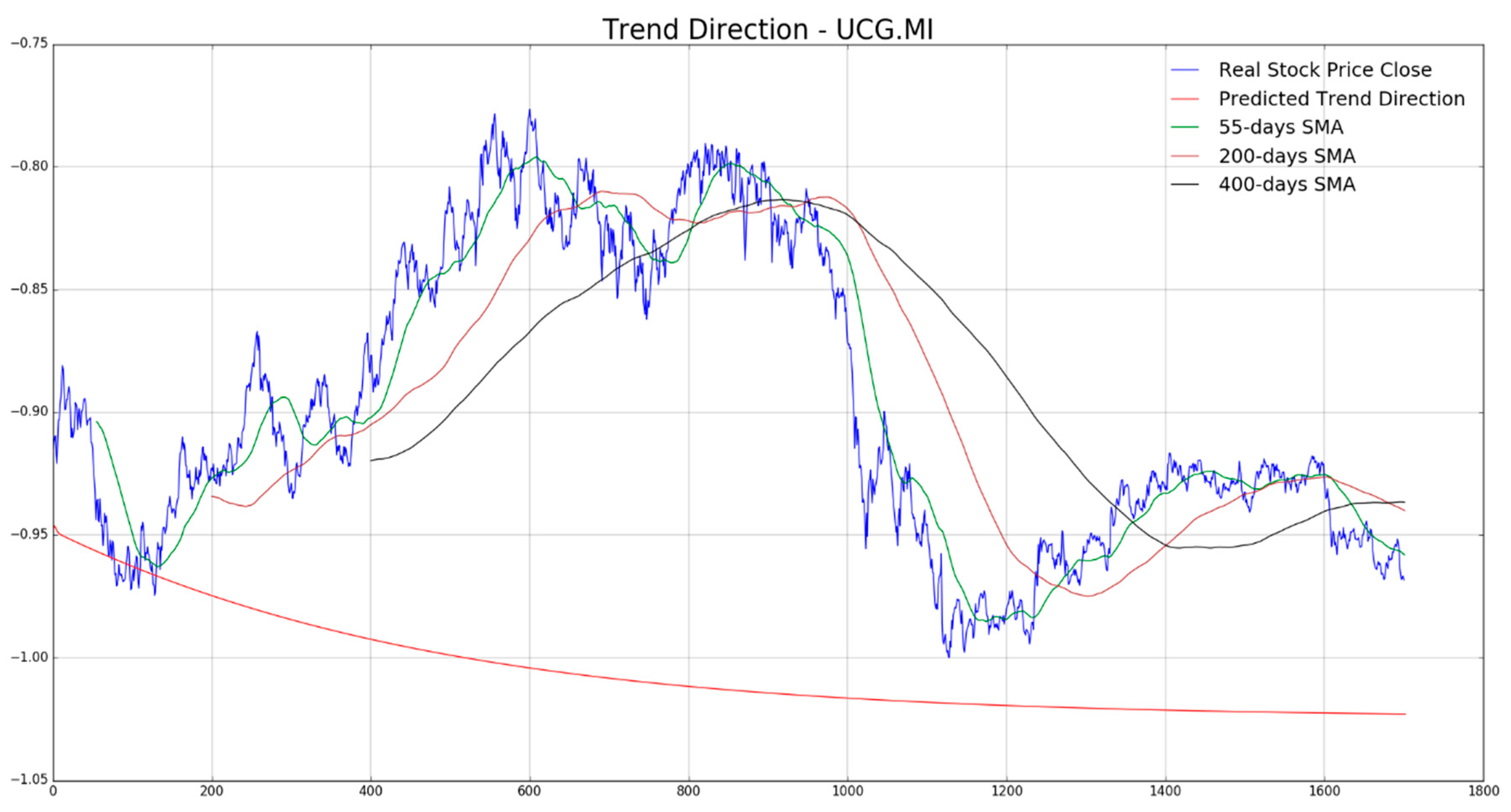
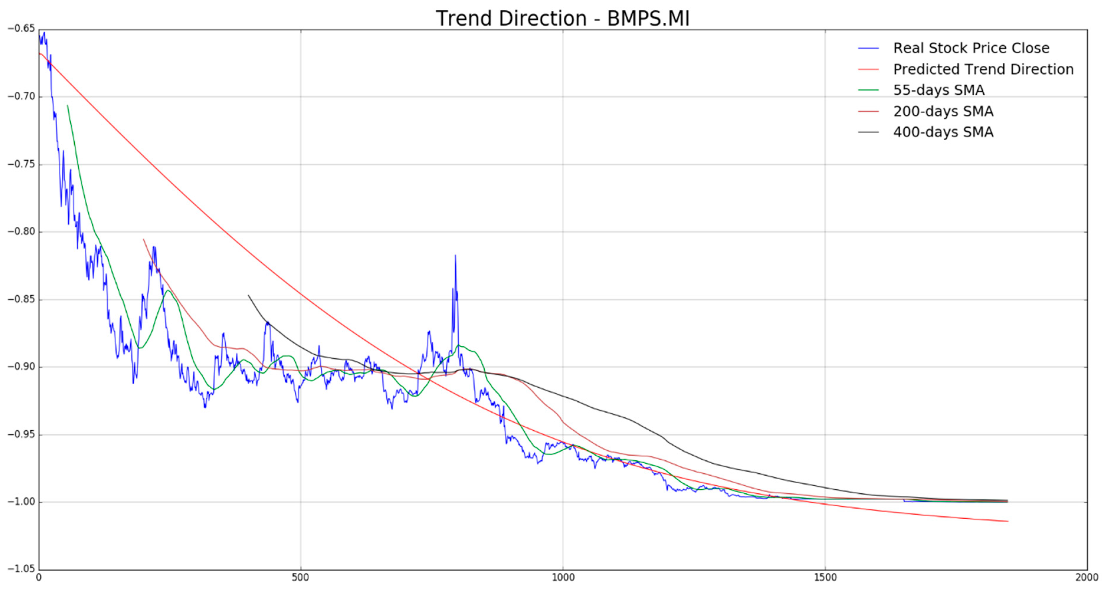
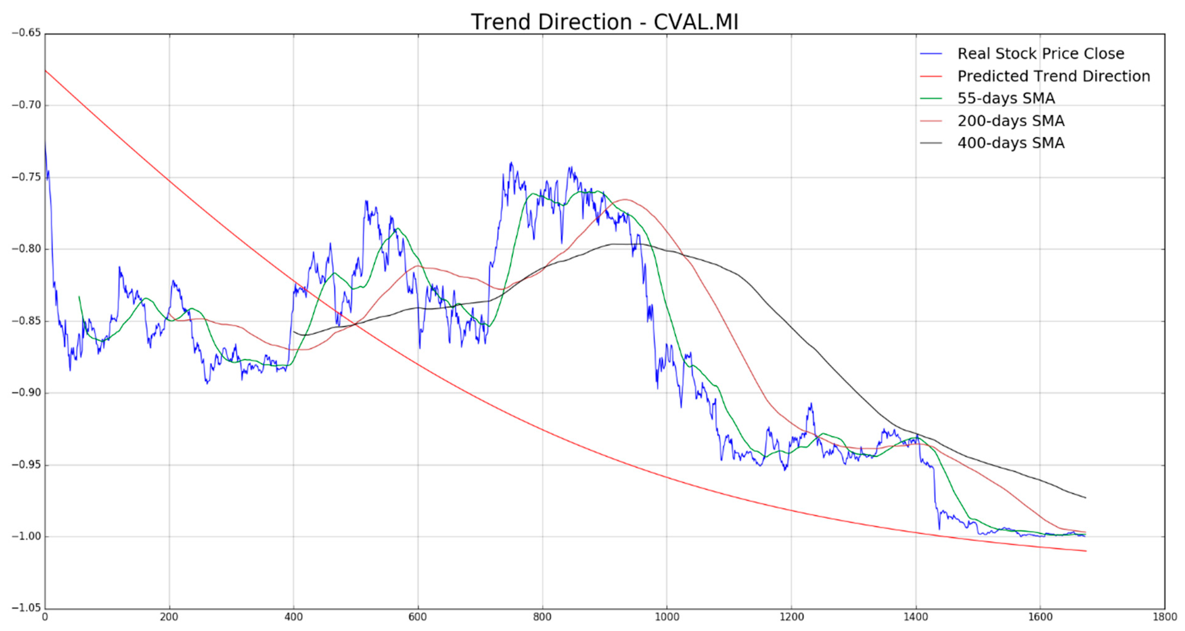
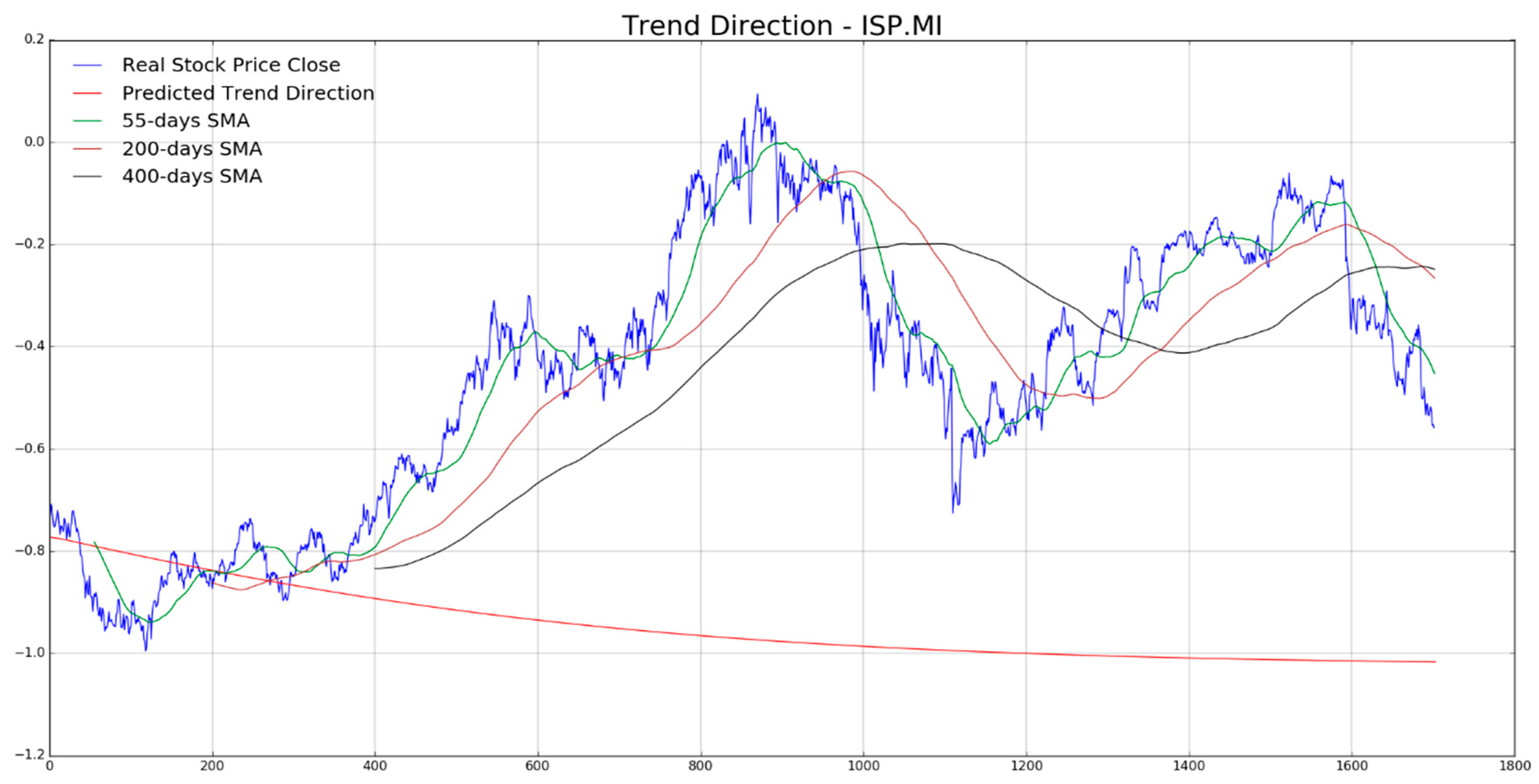
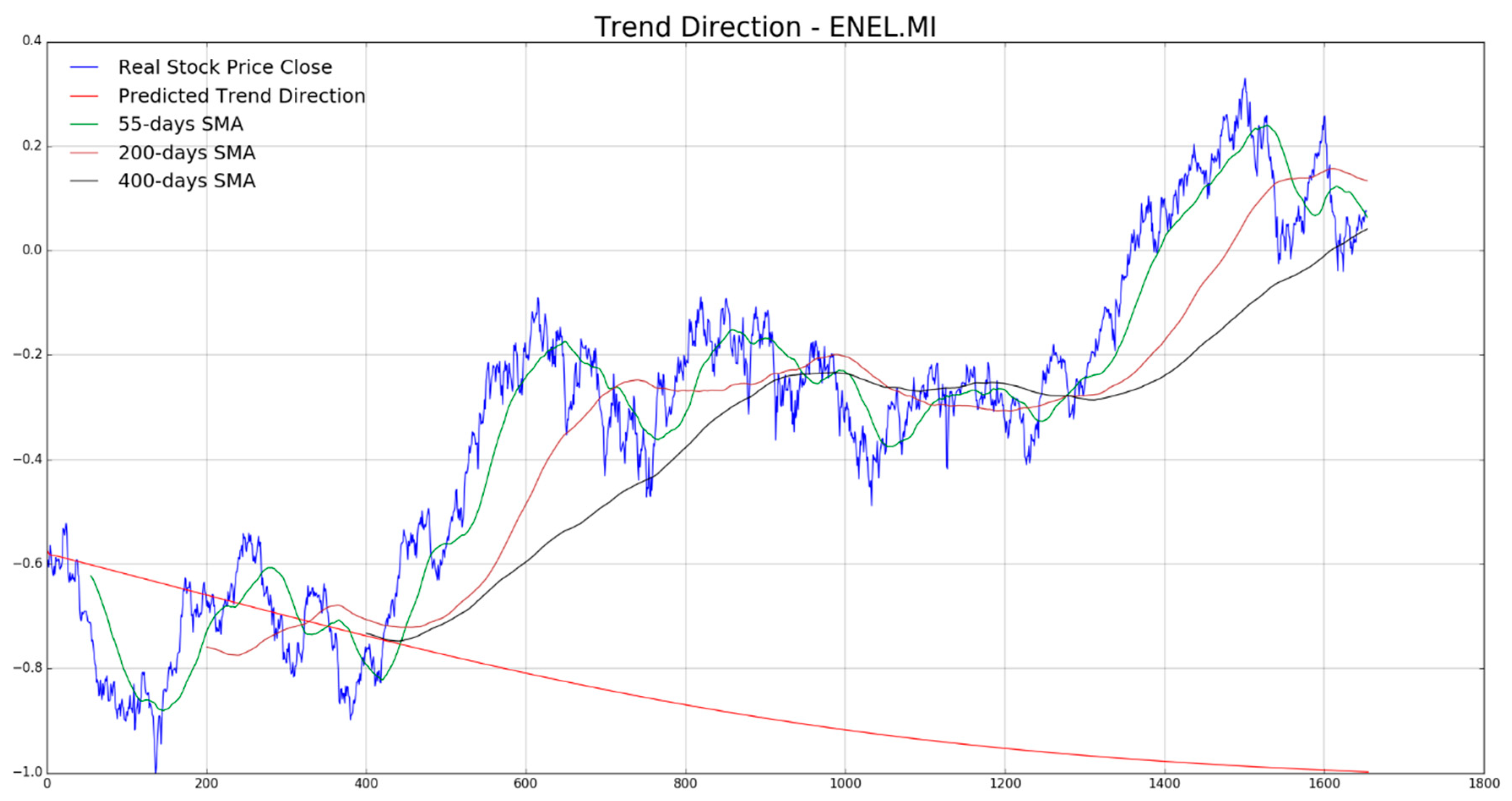
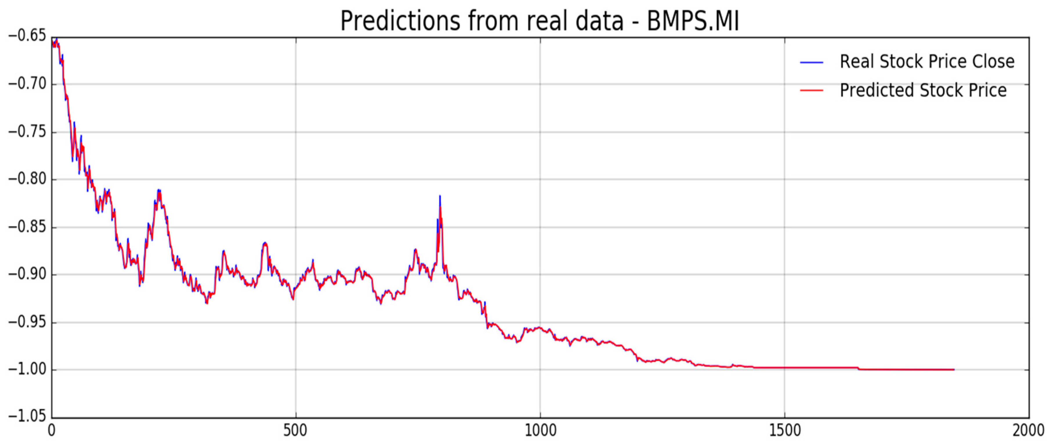
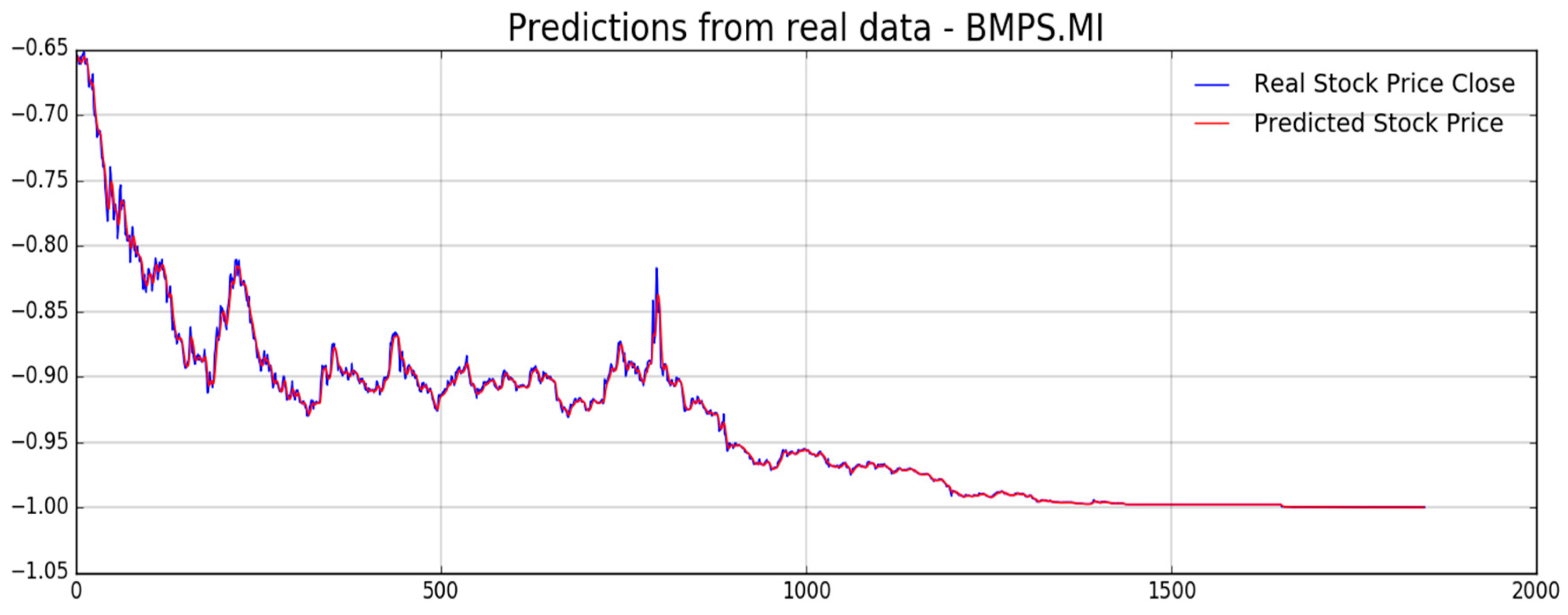
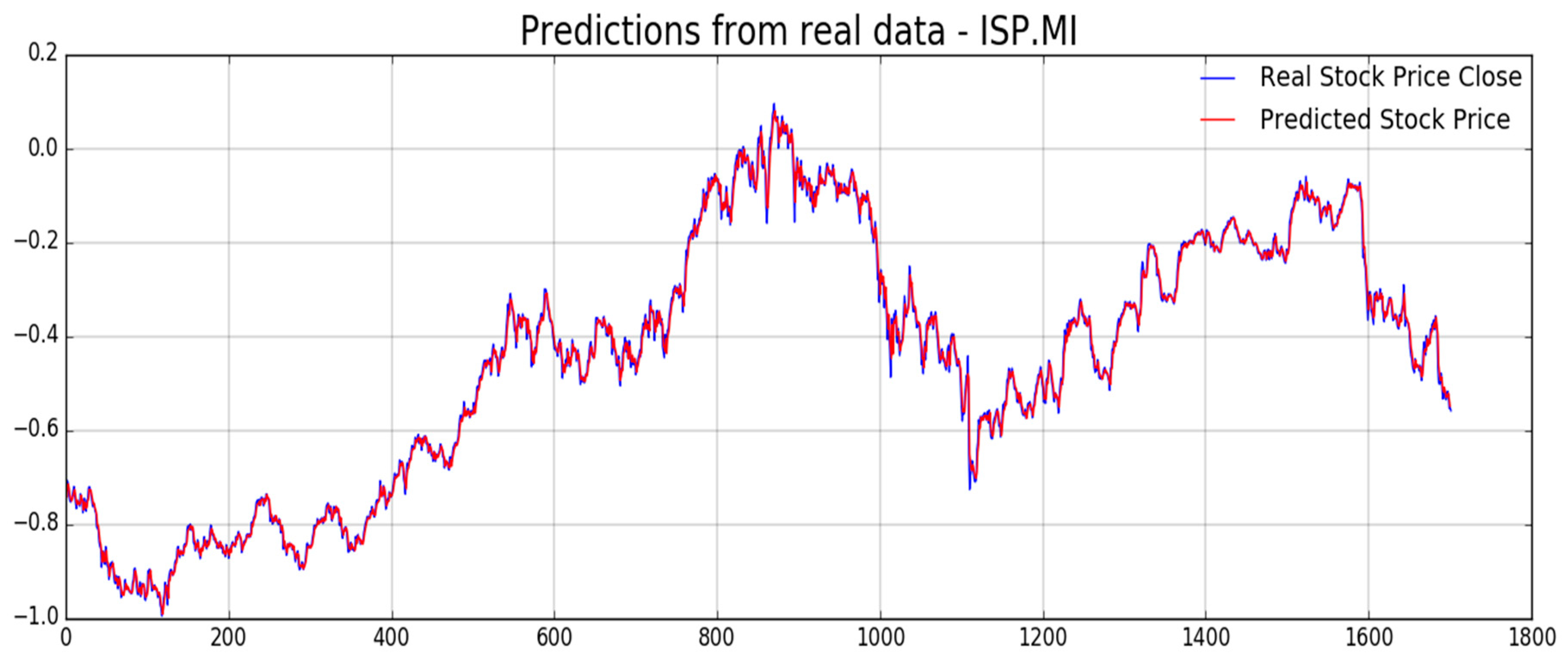
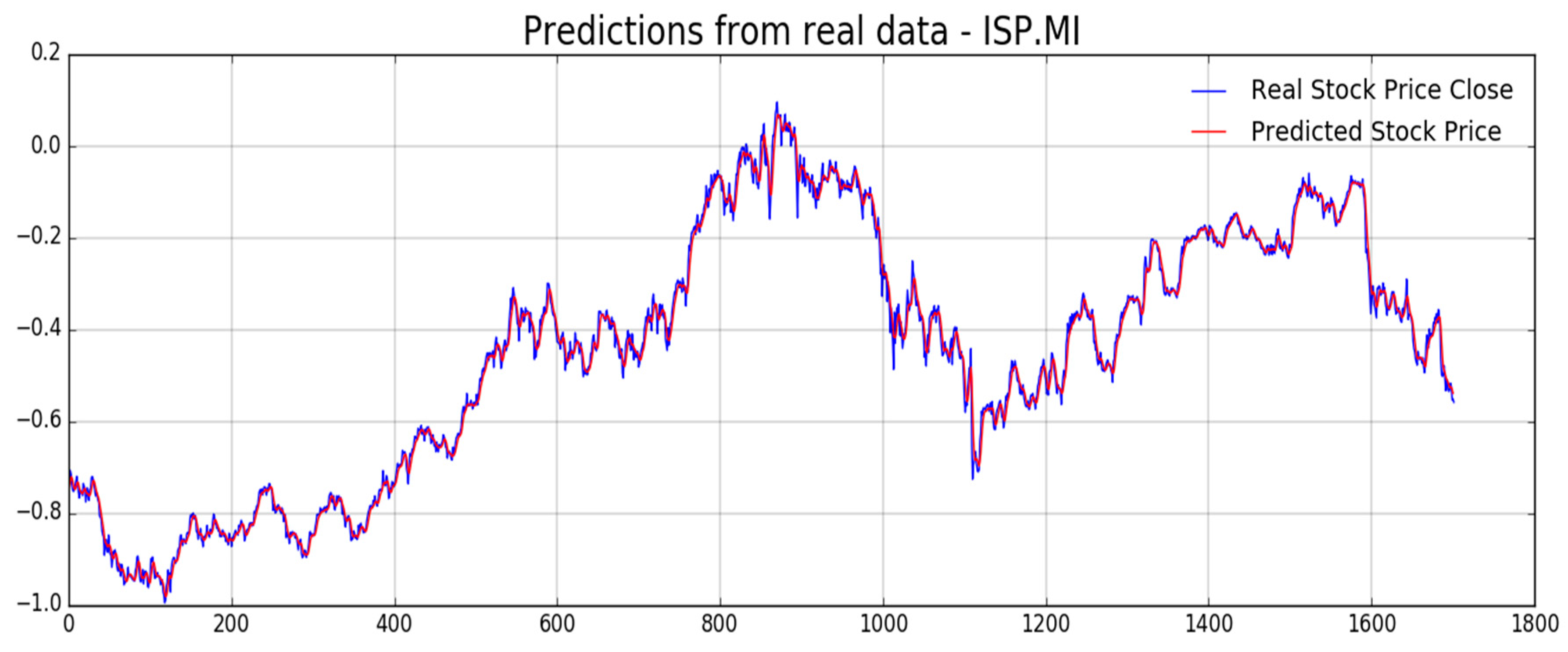
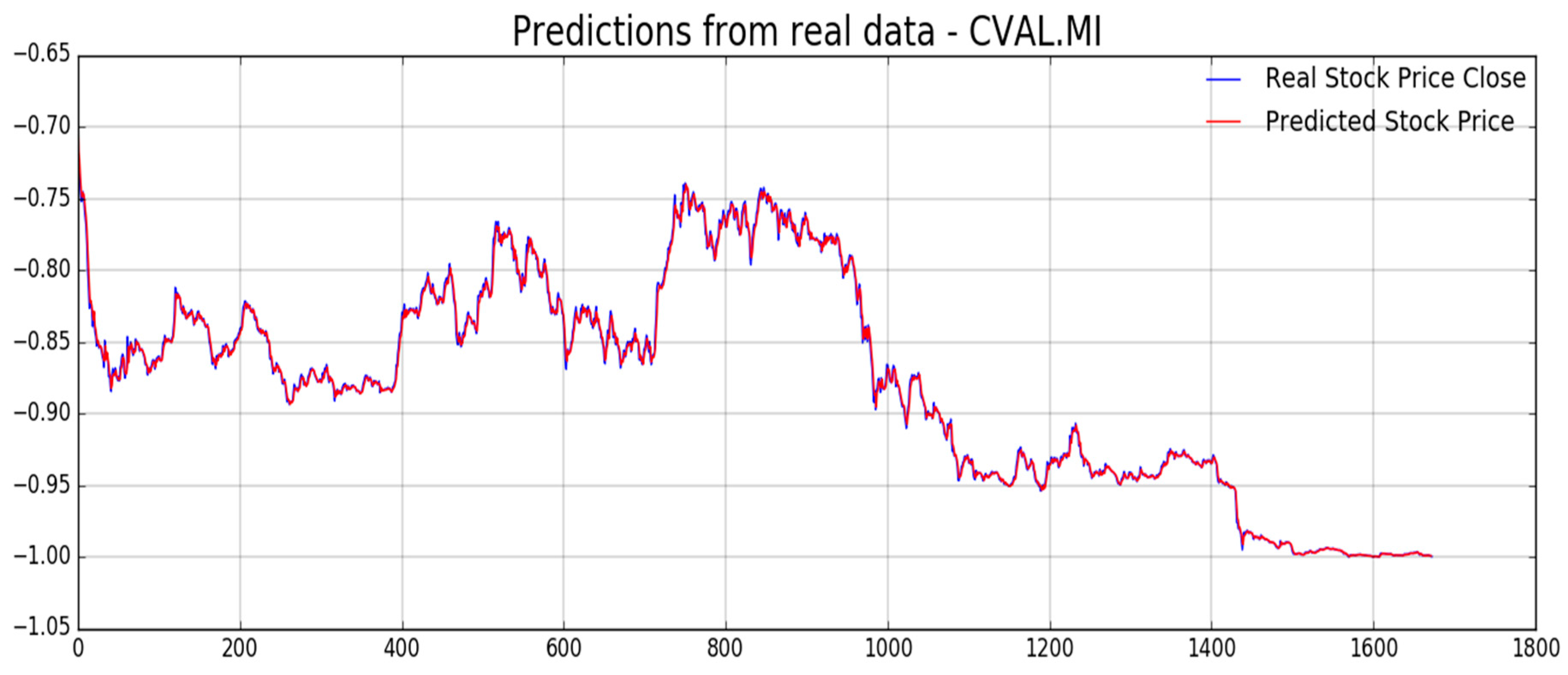
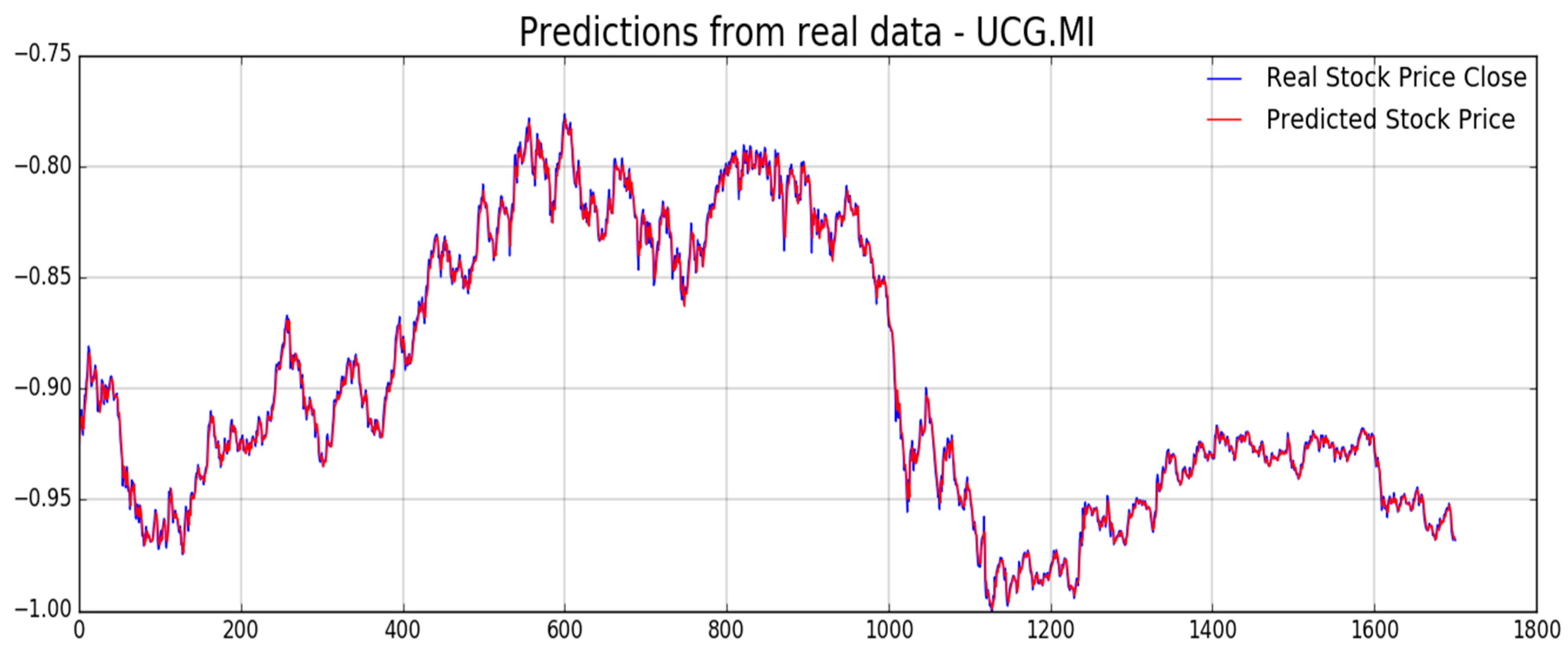
In Figure 7, Figure 8, Figure 9, Figure 10 and Figure 11 the authors report, for each diagram, the real stock trend (blue time-serie) with the predicted trend-line (red curve). For the sake of comparison, we reported such common mathematical heuristic financial indicator such as the Simple Moving Average (SMA) over different periods in order to perform a correct discrimination of the medium and long-term stock trend. As is well known, prediction of the stock price trend, especially mid-long term trend prediction, is a great challenge as per the complexity of that market usually affected by chaotic and unpredictable dynamics. For the reasons previously described, a zero-fault pipeline that is able to predict stock trend is very difficult to obtain. In that field, the proposed approach shows promising results even though there is, of course, a great amount of work to be done for improving the obtained performance in trend prediction. In our experiments, we have noted that for such stock the mid-long term trend prediction seems accurate (see Figure 8 and Figure 9), while the remaining ones (Figure 7, Figure 10, and Figure 11) shows a real trend not very compliant with the predicted ones likely due to such financial complex dynamic and market information not yet included in the LSTM learning, which is basically based to price movement dynamic only. Anyway, the trading system we have described in Section 4, is able to compensate the above displacements in trend prediction, as confirmed by the good results we report in the following figures. As described in the previous Figure 5, the proposed pipeline includes another LSTM based block for stock price prediction. In the next Figure 12, Figure 13, Figure 14, Figure 15, Figure 16 and Figure 17, we report experimental results we obtained on forecasting analyzed stocks time series (close price) by means of second LSTM layer with prediction price correction based on the assumption of that share price formation satisfies Markov propriety. In order to show the advantages of the proposed Markov-based price prediction correction with respect to classical LSTM based prediction system, in Figure 13 and Figure 15 the authors show the same stock price prediction reported in Figure 12 and Figure 14, respectively, but without the described Markov-based correction. Moreover, we report such benchmark comparisons for showing the robustness and effectiveness of the proposed prediction pipeline.
As previously mentioned, one of the challenging target for the pipeline herein described is to provide an efficient mechanism for stock price prediction. The proposed method shows satisfactory results when doing shares price forecasting so that we decided to report such type of numerical metrics in order to exhibit the proper benchmark comparison of that capability.
The analyzed stock price prediction benchmark metrics are reported in Table 1 and Table 2. More in detail, in Table 1, we report the average Root Mean Square Error (RMSE) for the single analyzed stock both in case of we apply the correction based on the assumption of price formation satisfies Markov propriety (RMSEupdate) and without that correction, i.e., as it is performed by the trained LSTM only. From a simple analysis of the data reported in Table 1, the assumption made by the author improves, significantly, the overall prediction performance of the proposed approach. In Table 2, the authors report a further statistical comparisons index: The variance computed for the target stock price, as well as for the corresponding predicted ones (both with proposed Markov based correction “update” —and without that- “no update”), for each analyzed stock, in order to confirm how effective is our prediction model. As for Table 1, Table 2 reported statistic evaluations, confirm the robustness of the proposed approach. The benchmarks reported in Table 1 and Table 2 provide such statistic comparisons related to stock price forecasting. In order to improve that benchmark comparisons, we decided to evaluate the performance of the proposed approach by means of common robust indexes used in scientific literature for this purpose. The first comparison index we have used is described in Reference [18] where the authors presented an innovative LSTM-based approach to predict financial indexes with comparable prediction errors. In Reference [18], the authors showed an interesting benchmark comparison index suitable to evaluate the stock price prediction accuracy. In order to evaluate the proposed prediction algorithm of ups (LONG trend also knows as “Bullish”) and downs (SHORT trend also known as “Bearish”), the authors decided to calculate data accuracy by using the set of equation reported in Equations (16) and (17).
where , represents the real share price at time i and i + 1 respectively and, than, represents the actual financial trend of the analyzed stock. We apply the same clustering as per Equation (16) to the set of predicted values. Obviously, the term (1: if the predicted trend is correct 0: otherwise) represents an average benchmark metric of the predicted trends.
The accuracy reached by authors in Reference [18] is in the range between 43% and 58% applied in the Shanghai Eastern market. The prediction accuracy of the proposed method is reported in Table 3. With a benchmark DA index in the range 50% to 99% our method confirms the robustness and the efficiency on stock price prediction.
At the end, the authors provide a further robustness benchmarks usually used in the financial market, i.e., the si called drawdown. It is so defined in Reference [19]: “A drawdown is the peak-to-trough decline during a specific recorded period of an investment, fund or commodity security. A drawdown is usually quoted as the percentage between the peak and the subsequent trough.” We performed a drawdown measure check of the proposed pipeline. The results are reported in Table 4.
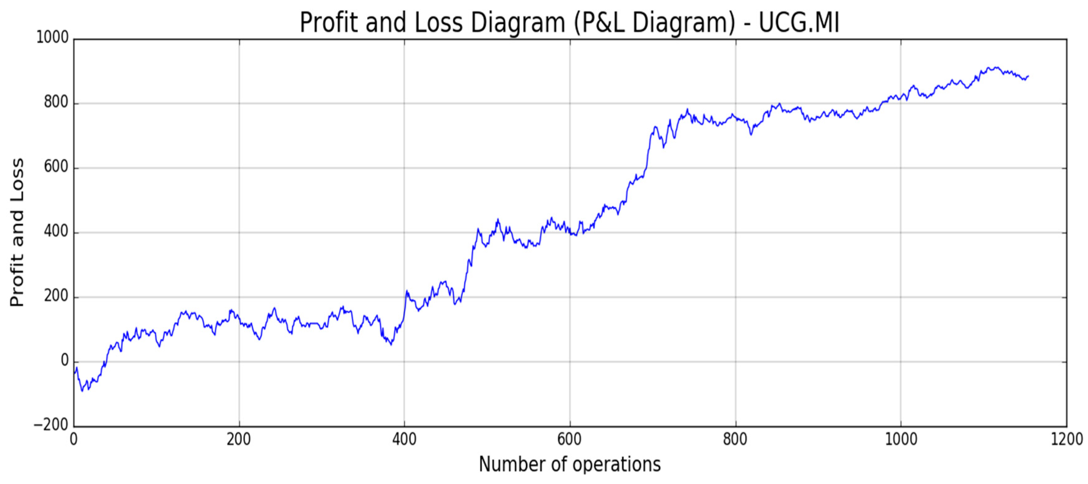
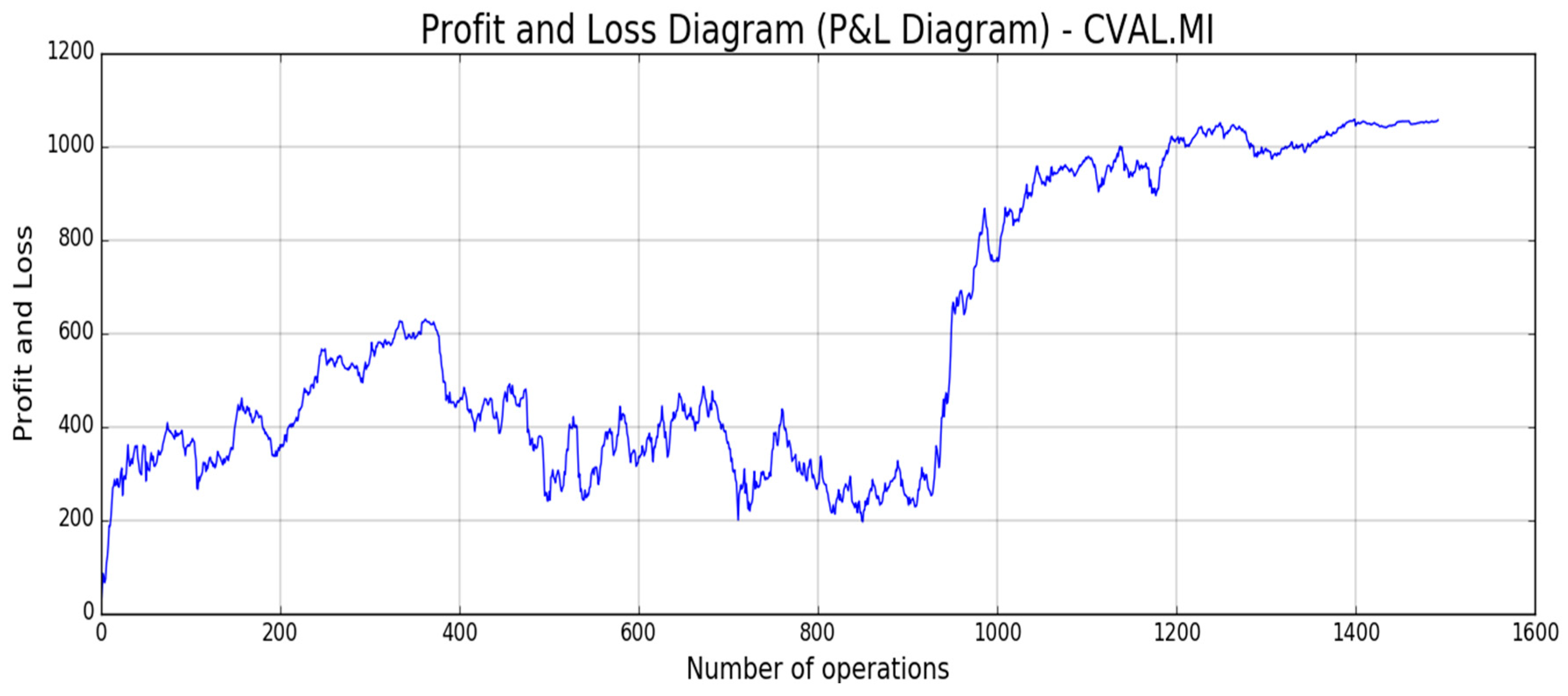
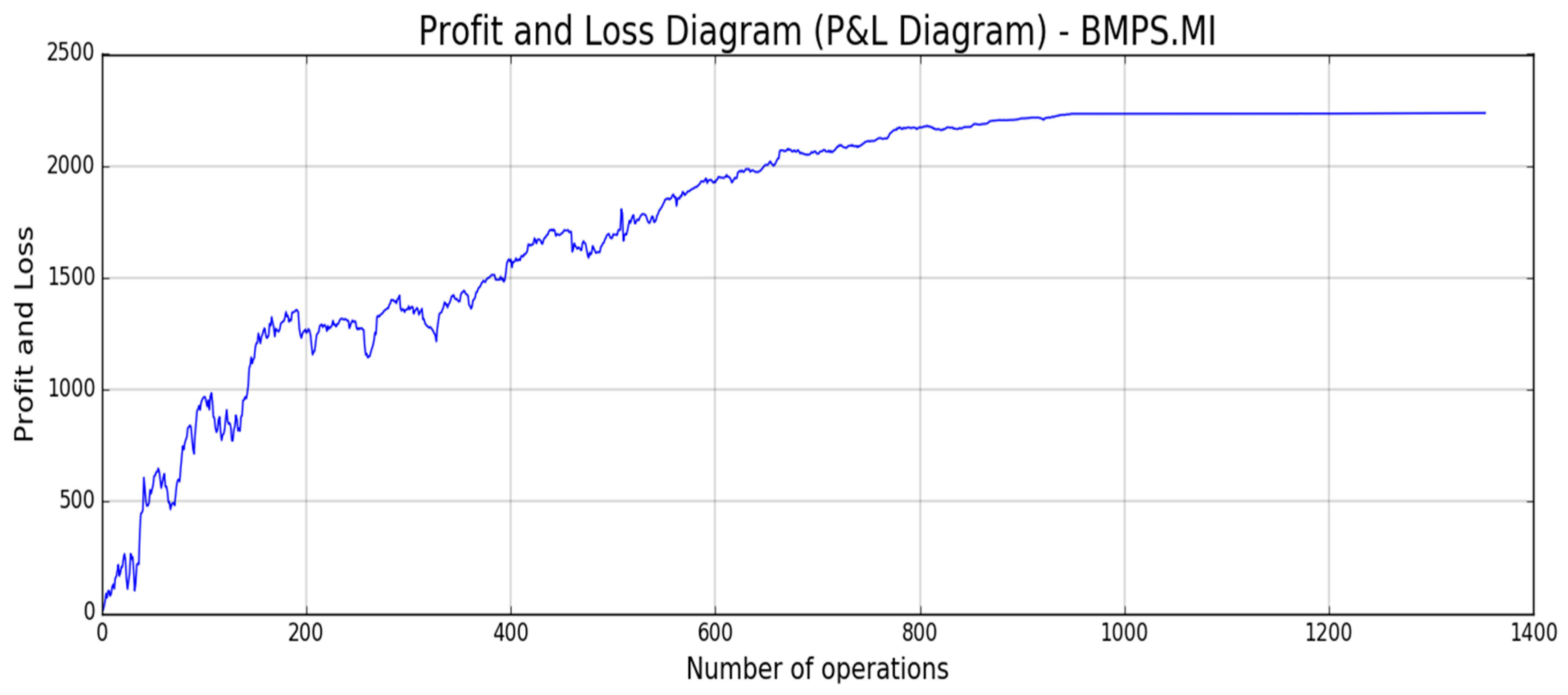
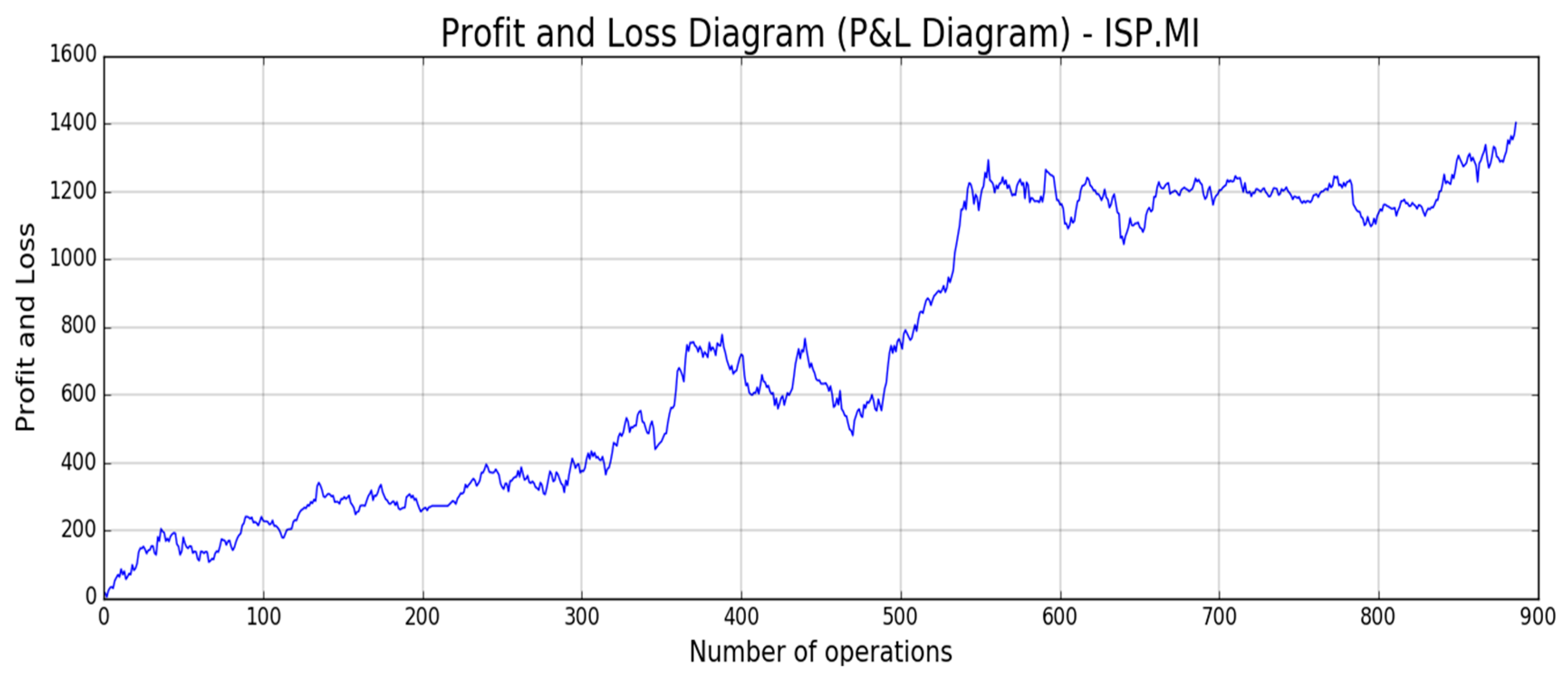
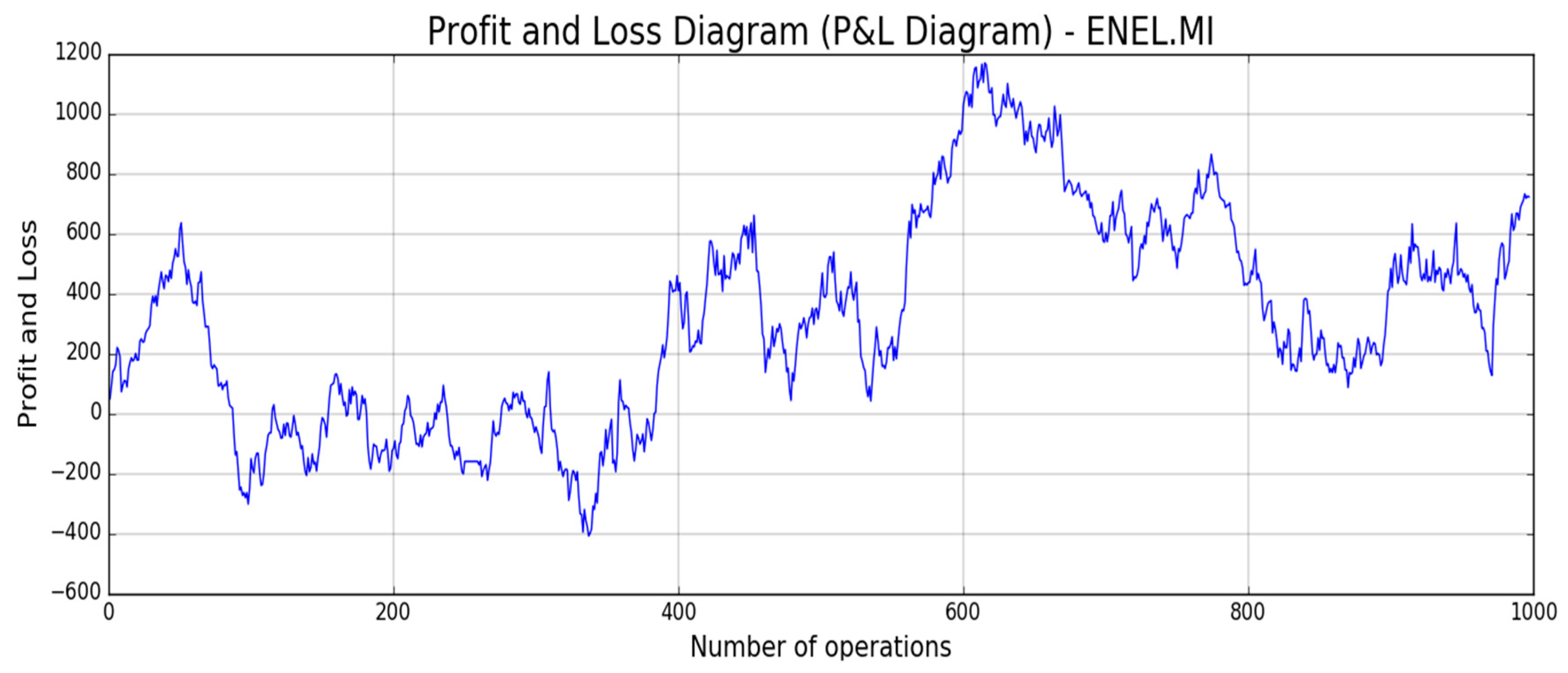
If we compare Maximum Drawdown results reported in Table 4 with similar ones reported in a recent algorithm based on Machine Learning technique [20], we easily understand that our proposed approach shows acceptable drawdown as it exposes almost 11 % of the total amount of investment which is a very promising result in the field of financial sustainable trading system [20]. Finally, the results we have obtained in stock price prediction by means of the proposed pipeline confirms the robustness and the effectiveness of the approach are herein described, getting up the overall accuracy of the proposed prediction system based on the LSTM only. The benchmark comparison reported in Table 1, Table 2, Table 3 and Table 4 confirms the mentioned advantages. Now, in order to validate the performance of the overall proposed system including the trading pipeline block, we have applied, as described in the previous section, our proposed pipeline for trading several stocks in the Milan Stocks Exchange Market. In Figure 18, Figure 19, Figure 20, Figure 21 and Figure 22, the reported results of classical Profit and Loss Diagram (P&L) computed in EURO currency (y axes) are shown.
The above figures show a very promising P/L trend with an encouraging profit trend-line together with a contained drawdown as reported in Table 4. Both results obtained for such different stocks confirm the robustness and the effectiveness of the proposed approach because it is able to find a good trade-off between profit and risk as the maximum drawdown is really sustainable for this type of investment.
6. Conclusions and Future Works
In this paper, we presented a Markov Propriety-based machine learning method for stock price close prediction with related trading system. Specifically, we implemented a robust algorithm for the stock trend and price prediction by using LSTM neural networks to show that Machine Learning is very effective to extract useful information from stock market. The contribution of our work reaches multiple goals. Firstly, we defined a proper stochastic method to improve the accuracy of the LSTM prediction capability (by means of the used Markov based correction). Moreover, we have used LSTM capability to add more information about mid-long term trend. In this way, we have improved drastically the robustness of the proposed approach as well as we have reduced, significantly, the risk of the single trade as the system performs the financial operations under appropriate conditions (same direction between predicted trend and opened trade). The applications in which the proposed method can be applied are really so many and they can go beyond the financial market field. We want to apply the proposed pipeline for improving trading system profitability of many banking and financial institutions, as well as for stock and financial indexes forecasting because those predicted data are often used for company market analysis or for taking main decisions in the field of economic and monetary policy. In order to improve the availability of the proposed approach, the authors are working to port the proposed algorithms within the STM32 based embedded platform [21] in order to have a standalone device for performing the aforementioned market analysis. Anyway, the proposed approach may be further improved in terms of predication capability and profitability. For this reason, the authors are evaluating such bio-inspired algorithms successfully used in some medical applications [22,23,24] for extracting ad-hoc features from financial time-series. The preliminary results are very encouraging and we hope to present such results in a following work. As previously reported, a methodology that could improve significantly the prediction capability of the proposed approach is based on social sentiment analysis, as described in Reference [8]. The authors observed that sentiment signals can influence the market price movements. An idea on which the authors are working consists in considering daily news in order to predict the stock pricing. Preliminary results confirm that this strategy can drastically improve the overall stock price and trend predictability. According to the results herein obtained, ad-hoc financial sentiment analysis algorithm is being developed to be added to our pipeline in order to improve the overall profitability and predictability of the proposed pipeline. Future works will focalize on intelligent integration between the analytic pipelines, herein described with sentiment analysis ones. One of the most recent work about this topic is described in Reference [25] from which the authors is started for current development.
Author Contributions
Conceptualization & Investigation, F.R.; Validation, F.T.; Writing-Review & Editing, S.B. and A.L.D.S.
Funding
This research received no external funding.
Conflicts of Interest
The authors declare no conflicts of interest.
References
- Kim, K.; Han, I. Genetic Algorithms Approach to Feature Discretization in Artificial Neural Networks for the prediction of Stock Price Index. Expert Syst. Appl. 2000, 19, 125–132. [Google Scholar] [CrossRef]
- Kimoto, T.; Asakawa, K.; Yoda, M. Stock Market Prediction System with Modular Neural Networks. In Proceedings of the 1990 IJCNN International Joint Conference on Neural Networks, San Diego, CA, USA, 17–21 June 1990. [Google Scholar]
- Wang, J.-H.; Leu, J.-Y. Stock market trend prediction using ARIMA-based neural networks. In Proceedings of the International Conference on Neural Networks (ICNN’96), Washington, DC, USA, 3–6 June 1996. [Google Scholar]
- Niaki, S.T.A.; Hoseinzade, S. Forecasting s&p 500 index using artificial neural networks and design of experiments. J. Ind. Eng. Int. 2013, 9, 1. [Google Scholar]
- Nelson, D.M.Q.; Pereira, A.C.M.; de Oliveira, R.A. Stock market’s price movement prediction with LSTM neural networks. In Proceedings of the 2017 International Joint Conference on Neural Networks (IJCNN), Anchorage, AK, USA, 14–19 May 2017. [Google Scholar]
- Zhang, Z.; Shen, Y.; Zhang, G.; Song, Y.; Zhu, Y. Short-term Prediction for Opening Price of Stock Market Based on Self-adapting Variant PSO-Elman Neural Network. In Proceedings of the 2017 8th IEEE International Conference on Software Engineering and Service Science (ICSESS), Beijing, China, 24–26 November 2017. [Google Scholar]
- Kumar, I.; Dogra, K.; Utreja, C.; Yadav, P. A Comparative study of supervised machine learning algorithms for stock market trend prediction. In Proceedings of the 2018 Second International Conference on Inventive Communication and Computational Technologies (ICICCT), Coimbatore, India, 20–21 April 2018. [Google Scholar]
- Bollen, J.; Mao, H. Twitter mood as a stock market predictor. Computer 2011, 44, 91–94. [Google Scholar] [CrossRef]
- Gers, F.A.; Schmidhuber, J. LSTM Recurrent Neural Networks Learn Simple Context Free and Context Sensitive Languages. IEEE Trans. Neural Netw. 2001, 12, 1333–1340. [Google Scholar] [CrossRef] [PubMed]
- Diebold, F.X. Elements of Forecasting, 4th ed.; Thomson Learning: Belmont, CA, USA, 2007. [Google Scholar]
- Granger, C.; Newbold, P. Forecasting Transformed Series. J. R. Stat. Soc. 2001, 38, 189–203. [Google Scholar] [CrossRef]
- Gers, F.A.; Schraudolph, N.N.; Schmidhuber, J. Learning precise timing with LSTM recurrent networks. J. Mach. Learn. Res. 2003, 3, 115–143. [Google Scholar]
- Savvopoulos, A.; Kanavos, A.; Mylonas, P.; Sioutas, S. LSTM Accelerator for Convolutional Object Identification. Algorithms 2018, 11, 157. [Google Scholar] [CrossRef]
- Yahoo Finance. Available online: https://it.finance.yahoo.com/ (accessed on 24 October 2018).
- Somani, P.; Talele, S.; Sawant, S. Stock Market Prediction Using Hidden Markov Model. In Proceedings of the 7th Joint International Information Technology and Artificial Intelligence Conference, Chongqing, China, 20–21 December 2014. [Google Scholar]
- Keras Documentation. Available online: https://keras.io/ (accessed on 24 October 2018).
- Tensorflow.org. Available online: https://www.tensorflow.org/ (accessed on 24 October 2018).
- Pang, X.; Zhou, Y.; Wang, P.; Lin, W.; Chang, V. An innovative neural network approach for stock market prediction. J. Supercomput. 2018, 1–21. [Google Scholar] [CrossRef]
- Investopedia. Available online: https://www.investopedia.com/terms/d/drawdown.asp (accessed on 17 December 2018).
- Reid, D.; Hussain, A.J.; Tawfik, H. Spiking Neural Networks for Financial Data Prediction. In Proceedings of the 2013 International Joint Conference on Neural Networks (IJCNN), Dallas, TX, USA, 4–9 August 2013. [Google Scholar]
- Artificial Intelligence (AI)—STMicroelectronics. Available online: https://www.st.com/content/st_com/en/about/innovation---technology/artificial-intelligence.html (accessed on 17 December 2018).
- Rundo, F.; Conoci, S.; Ortis, A.; Battiato, S. An Advanced Bio-Inspired PhotoPlethysmoGraphy (PPG) and ECG Pattern Recognition System for Medical Assessment. Sensors 2018, 18, 405. [Google Scholar] [CrossRef] [PubMed]
- Rundo, F.; Ortis, A.; Battiato, S.; Conoci, S. Advanced Bio-Inspired System for Noninvasive Cuff-Less Blood Pressure Estimation from Physiological Signal Analysis. Computation 2018, 6, 46. [Google Scholar] [CrossRef]
- Rundo, F.; Conoci, S.; Banna, G.L.; Ortis, A.; Stanco, F.; Battiato, S. Evaluation of Levenberg–Marquardt neural networks and stacked autoencoders clustering for skin lesion analysis, screening and follow-up. IET Comput. Vis. 2018, 12, 957–996. [Google Scholar] [CrossRef]
- Ortis, A.; Farinella, G.M.; Torrisi, G.; Battiato, S. Visual Sentiment Analysis Based on Objective Text Description of Images. In Proceedings of the International Conference on Content-Based Multimedia Indexing (CBMI), La Rochelle, France, 4–6 September 2018. [Google Scholar]
Figure 1.
Long Short-Term Memory (LSTM) model.

Figure 2.
Prototype LSTM cell.

Figure 3.
UCG.MI training and validation set.

Figure 4.
Overall scheme for the proposed stock trend/price prediction pipeline.

Figure 5.
Overall scheme of the whole proposed financial pipeline.

Figure 6.
Trading System Pipeline.

Figure 7.
UCG.MI Trend Direction (red) and SMA.

Figure 8.
BMPS.MI Trend Direction (red) and SMA.

Figure 9.
CVAL.MI Trend Direction (red) and SMA.

Figure 10.
ISP.MI Trend Direction (red) and SMA.

Figure 11.
ENEL.MI Trend Direction (red) and SMA.

Figure 12.
BMPS.MI Close Price time-serie (red: predicted; blue: real value).

Figure 13.
BMPS.MI Close Price time-serie (red: predicted without Markov correction; blue: real value).
Figure 13.
BMPS.MI Close Price time-serie (red: predicted without Markov correction; blue: real value).

Figure 14.
ISP.MI Close Price time-serie (red: predicted; blue: real value).

Figure 15.
ISP.MI Close Price time-serie (red: predicted without Markov correction; blue: real value).
Figure 15.
ISP.MI Close Price time-serie (red: predicted without Markov correction; blue: real value).

Figure 16.
CVAL.MI Close Price time-serie (red: predicted; blue: real value).

Figure 17.
UCG.MI Close Price time-serie (red: predicted; blue: real value).

Figure 18.
UCG.MI Profit and Loss Diagram.

Figure 19.
CVAL.MI Profit and Loss Diagram.

Figure 20.
BMPS.MI Profit and Loss Diagram.

Figure 21.
ISP.MI Profit and Loss Diagram.

Figure 22.
ENEL.MI Profit and Loss Diagram.


Table 1.
ENEL.MI, UCG.MI, BMPS.MI, CVAL.MI, and ISP.MI RMSE normalized in [0, 1] while enclosed in bracket corresponding not normalized.
Table 1.
ENEL.MI, UCG.MI, BMPS.MI, CVAL.MI, and ISP.MI RMSE normalized in [0, 1] while enclosed in bracket corresponding not normalized.
| ENEL.MI | UCG.MI | BMPS.MI | CVAL.MI | ISP.MI | |
|---|---|---|---|---|---|
| 0.030 (0.08132) | 0.0064 (0.75) | 0.0053 (30.0152) | 0.0067 (0.068) | 0.027 (0.06787) | |
| 0.028 (0.07633) | 0.0060 (0.70) | 0.0052 (28.069) | 0.0060 (0.064) | 0.025 (0.0631) |
Table 2.
ENEL.MI, UCG.MI, BMPS.MI, CVAL.MI, and ISP.MI Variance normalized in [0, 1] while enclosed in bracket corresponding not normalized
Table 2.
ENEL.MI, UCG.MI, BMPS.MI, CVAL.MI, and ISP.MI Variance normalized in [0, 1] while enclosed in bracket corresponding not normalized
| ENEL.MI | UCG.MI | BMPS.MI | CVAL.MI | ISP.MI | |
|---|---|---|---|---|---|
| 0.0923 (0.66) | 0.00362 (47,6) | 0.004569 (147786) | 0.0055 (0.27) | 0.0732 (0.4542) | |
| 0.092 (0.65) | 0.00357 (46.5) | 0.00463 (147812) | 0.0054 (0.2451) | 0.0729 (0.4504) | |
| 0.09221 (0.66) | 0.00360 (46.7) | 0.00462 (147619) | 0.0055 (0.2456) | 0.0730 (0.4509) |
Table 3.
ENEL.MI, UCG.MI, BMPS.MI, CVAL.MI, and ISP.MI Data Accuracy (DA) results.
| ENEL.MI | UCG.MI | BMPS.MI | CVAL.MI | ISP.MI | |
|---|---|---|---|---|---|
| 0.501813 | 0.999412 | 0.510281 | 0.99402 | 0.50 |
Table 4.
ENEL.MI, UCG.MI, BMPS.MI, CVAL.MI, and ISP.MI. Maximum Drawdown (%) results.
| ENEL.MI | UCG.MI | BMPS.MI | CVAL.MI | ISP.MI | |
|---|---|---|---|---|---|
| −9.2350 | −3.3345 | −11.0911 | −4.0011 | −10.9876 |
© 2019 by the authors. Licensee MDPI, Basel, Switzerland. This article is an open access article distributed under the terms and conditions of the Creative Commons Attribution (CC BY) license (http://creativecommons.org/licenses/by/4.0/).
Share and Cite
MDPI and ACS Style
Rundo, F.; Trenta, F.; Di Stallo, A.L.; Battiato, S. Advanced Markov-Based Machine Learning Framework for Making Adaptive Trading System. Computation 2019, 7, 4. https://0-doi-org.brum.beds.ac.uk/10.3390/computation7010004
AMA Style
Rundo F, Trenta F, Di Stallo AL, Battiato S. Advanced Markov-Based Machine Learning Framework for Making Adaptive Trading System. Computation. 2019; 7(1):4. https://0-doi-org.brum.beds.ac.uk/10.3390/computation7010004
Chicago/Turabian StyleRundo, Francesco, Francesca Trenta, Agatino Luigi Di Stallo, and Sebastiano Battiato. 2019. "Advanced Markov-Based Machine Learning Framework for Making Adaptive Trading System" Computation 7, no. 1: 4. https://0-doi-org.brum.beds.ac.uk/10.3390/computation7010004
Note that from the first issue of 2016, this journal uses article numbers instead of page numbers. See further details here.