Machine-Learning Prediction of Underwater Shock Loading on Structures

1
Beijing Institute of Space Long March Vehicle, Beijing 100076, China
2
University of Nicosia, Nicosia CY-2417, Cyprus
3
Department of Design, Manufacturing and Engineering Management, University of Strathclyde, Glasgow, G1 1XQ, UK
*
Author to whom correspondence should be addressed.
Computation 2019, 7(4), 58; https://0-doi-org.brum.beds.ac.uk/10.3390/computation7040058
Submission received: 15 August 2019
/
Revised: 16 September 2019
/
Accepted: 18 September 2019
/
Published: 8 October 2019
(This article belongs to the Special Issue Machine Learning for Computational Science and Engineering)
Abstract
:Due to the complex physics of underwater explosion problems, it is difficult to derive analytical solutions with accurate results. In this study, a machine-learning method to train a back-propagation neural network for parameter prediction is presented for the first time in literature. The specific problem is the response of a structure submerged in water subjected to shock loads produced by an underwater explosion, with the detonation point being far away from the structure so that the loading wave can be regarded as a planar shock wave. Two rigid parallel plates connected by a linear spring and a linear dashpot that simulate structural stiffness and damping respectively, represent the structure. Taking the Laplace transform of the governing equations, solving the resulting equations, and then taking the inverse Laplace transform, the simplified problem is analyzed theoretically. The coupled ordinary differential equations governing the motion of the system are also solved numerically by the fourth order Runge–Kutta method and then verified by a finite element method using Ansys/LSDYNA. The parametric training with the back-propagation neural network algorithm was conducted to delineate the effects of structural stiffness and damping on the attenuation of shock waves, the cavitation time, and the time of maximum momentum transfer. The prediction results agree well with the validation and test sample results.
1. Introduction
Taylor [1] presented a closed form solution for the response of an infinite rigid flat plate, with the back face connected to a linear spring, the front face immersed in water, and exposed to an exponentially decaying plane shock wave. It was shown that the peak momentum transmitted to a free-standing plate decreases significantly with increasing fluid–structure interaction (FSI) effects.
Taylor’s analysis of the plane shock wave impinging upon an air-backed plate (ABP) was recently extended to a submerged water-backed plate (WBP) by Liu and Young [2]. It is shown that the WBP experiences lower pressure load, and thus has a lower peak momentum than an equivalent ABP. The extension of Taylor’s work for air blast loading was accomplished in [3,4,5] where the importance of nonlinear compressibility effects has been delineated [6]. Hutchinson and Xue [7,8] numerically solved the FSI problem using the commercial software Ansys/LSDYNA [9] and accounted for the yield strength of the core to improve the estimate of the momentum transmitted to a sandwich structure.
The time for the linear momentum of the plate to reach its peak value is shorter for the WBP than that for the ABP, and cavitation is found to be almost inevitable for the ABP, but occurs for the WBP only for a small range of values of the FSI parameter.
In addition to Taylor-type models, other analytical works have investigated the dynamic response of elastic shells subjected to underwater shock loading [10,11,12,13,14,15,16]. Here, the analysis of Taylor’s ABP and Liu and Young’s WBP are extended to include the effects of structural stiffness and damping by modelling the FSI problem as a system of two parallel infinite rigid flat plates interconnected by a spring and a dashpot, with the right plate exposed to an exponentially decaying planar wave. The whole system may be immersed in water, or only the left plate is immersed in water and the right plate is exposed to air. The goal is to quantify the effects of structural strength on its deformations due to a planar shock wave.
2. Formulation of the Problem
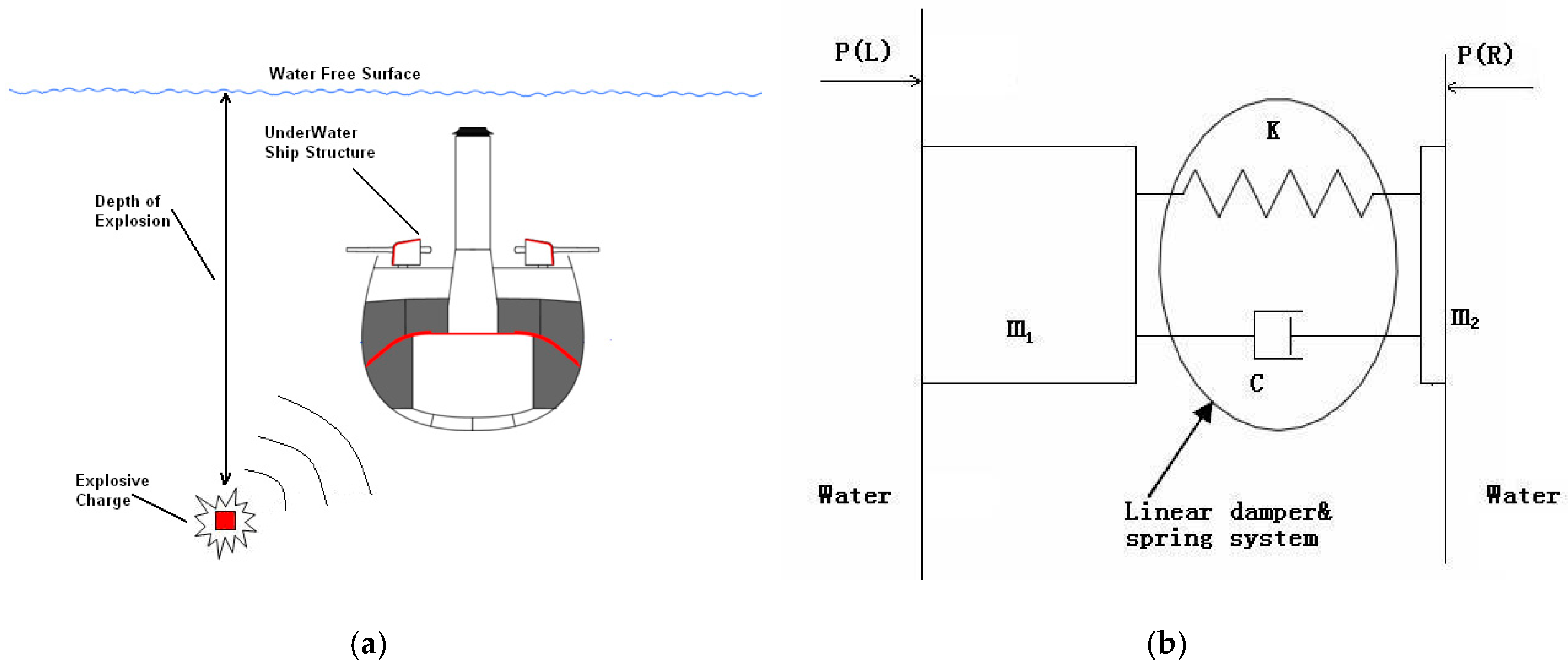
The problem, depicted schematically in Figure 1a, is analyzed. It shows a marine vessel partially immersed in water and an explosive device detonated at a point far away from it. A simple model for studying deformations of the marine vessel subjected to a shock wave produced by the detonation of the explosive device is shown in Figure 1b. For estimating the effects of the structural stiffness and its damping on the transmission and reflection of the incident wave, the problem is simplified considerably by modelling the structure as two infinite parallel rigid plates interconnected by a linear spring and a linear dashpot as shown in Figure 1. The incident wave and the wave reflected from the left plate travel in water, but the wave emanating from the right plate may propagate either into water or into air.
2.1. Governing Equations
The mass per unit area of each plate is denoted by m= ρshs where ρs and hs are the mass density (mass/volume) and thickness of the plate, respectively. We also use a rectangular Cartesian coordinate system with the origin at the left plate to describe deformations of the system. A plane incident wave traveling along the x-axis with pressure given by
strikes the left flat rigid plate ΩL at time t = 0; c is the speed of sound in water; P0 is the peak pressure and θ is the pressure decay time. The plate can freely travel along the x-axis (which is from left to right side). The wave is partly reflected back into water and is partly transmitted to the right plate through the spring and the dashpot. Thus, the net pressure on ΩL equals the sum of the pressure from the incident wave and the pressure
from the reflected wave. The function is to be determined. Let , , and be the displacement, the velocity, and the acceleration, respectively, in the x-direction of ΩL. Assuming that water particles stay in contact with ΩL, then the water particles touching the plate also have an x-displacement equal to . The mass and the linear momentum balance near ΩL result in the particle velocity:
Combining (2) and (3) yields
for the net pressure acting on the left plate. If the left rigid plate was fixed, then the incident wave would be fully reflected, and the resultant pressure on it would be twice the pressure of the incident wave. However, the axial translation of the plate due to its connection to the right plate via a damper and a spring leads to a partial reflection of the incident wave, and the pressure reduction as compared to that on a fixed surface is . Similarly, the mass and the moment balance near the right rigid plate ΩR gives
where PR(t) is the pressure on the surface of ΩR not connected to the spring and the dashpot. Equations of motion of the left and the right plates are
where
subscripts 1 and 2 denote quantities for the left and the right rigid plates, respectively. Cdamp and k are the damping coefficient and the spring stiffness, respectively. Matrix forms (6) and (7) can be written as the following system of coupled ordinary linear differential equations.
2.2. Analytical Solution
The Laplace transform of function u(t) by U(s) is defined by
Taking the Laplace transform of (8), the resulting equations for U1(s) and U2(s) are solved as:
By taking the Laplace transform with the formula
the expressions for the displacement, the velocity, and the acceleration are obtained.
2.3. Numerical Solution
Equation (8) is also solved numerically using the fourth order Runge–Kutta method. Setting ; then a first order ordinary differential equation (ODE), for is written as follows:
3. Results of Structural Response
In order to investigate the influence of different parameters on the fluid–structure interaction (FSI) problem, the following are set: ρ = 1000 kg/m3, c = 1400 m/s, m1 = m2 = 80 kg/m2, P0 = 10 MPa, and decay time θ = 0.1 ms. Thus, ϕ1 = 2ρcθ/m1 = 3.5, ϕ2 = 2ρcθ/m2 = 3.5. Values of variables indicated in the Figures are in MKS (Meter-Kg-Seconds) units.
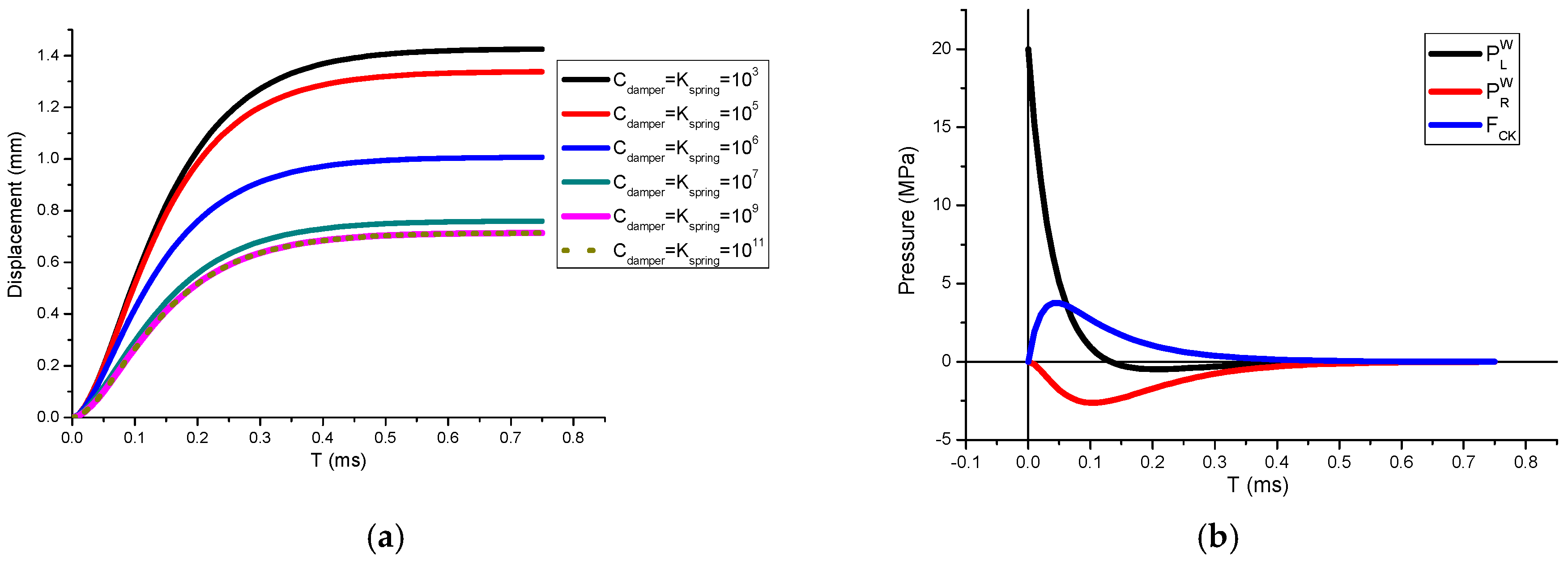
Figure 2a shows the effect of varying the structural stiffness k and the damping Cdamp on the time histories of the displacement of the left plate. As expected, increasing the values of k and Cdamp led to the peak plate deflection and the speed of the left plate decreasing. For values of k and Cdamp greater than 109, the structural response was equivalent to that of a rigid body of mass equal to m1 + m2, whereas values of k used herein were representative of those for a structure.
Time histories of the resultant pressure on the left and the right plates, and the interaction pressure between them, are exhibited in Figure 2b. At t = 0.13 ms, the resultant pressure on the left plate equals zero, implying that the fluid will separate from the plate, or equivalent cavitation will set in unless the fluid can support the tensile pressure. In the results shown in Figure 2b, the fluid is assumed not to separate from the plate.
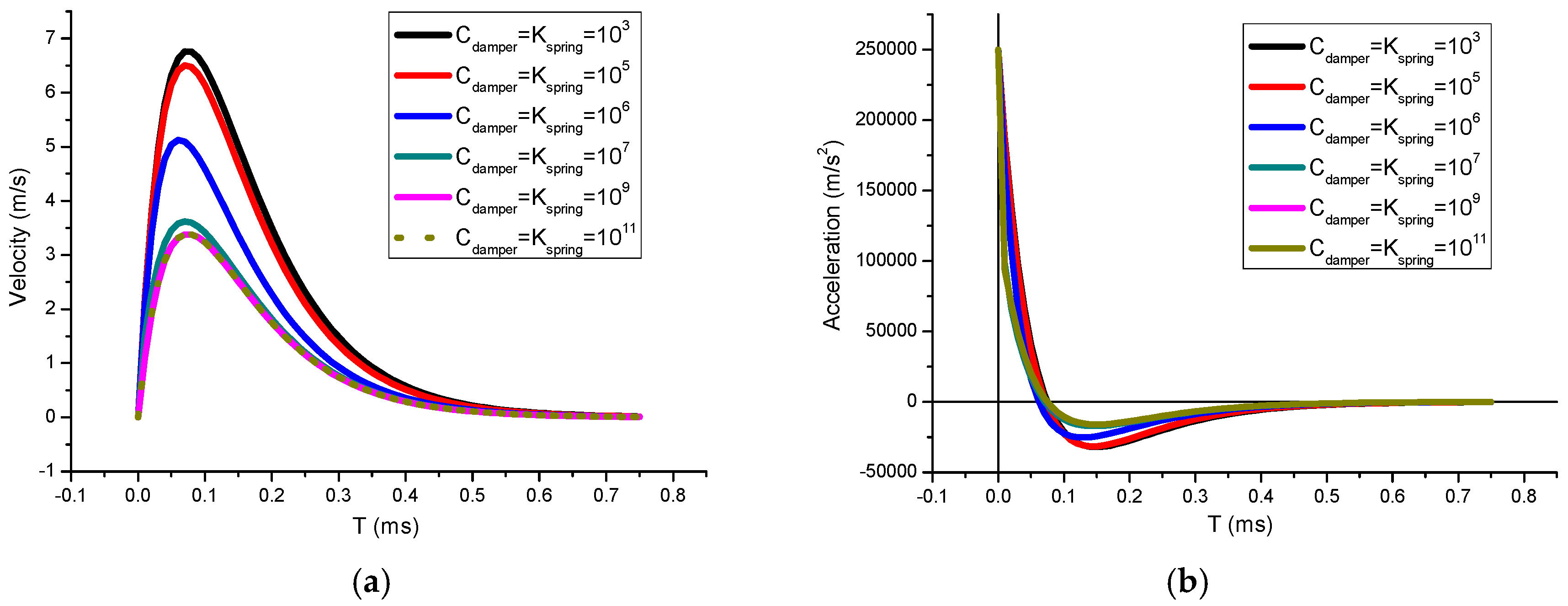
Time histories of the x-velocity and the x-acceleration of the left plate depicted in Figure 3 reveal that upon impact, the speed increased rapidly to its peak value in about 0.06 ms, and then gradually decreased. The time at which the speed took its maximum value was not influenced by the values of k and Cdamp. However, these parameters strongly affected the magnitude of the maximum speed of the left plate. Different values of k and Cdamp had relatively little effect on the acceleration of the left plate.
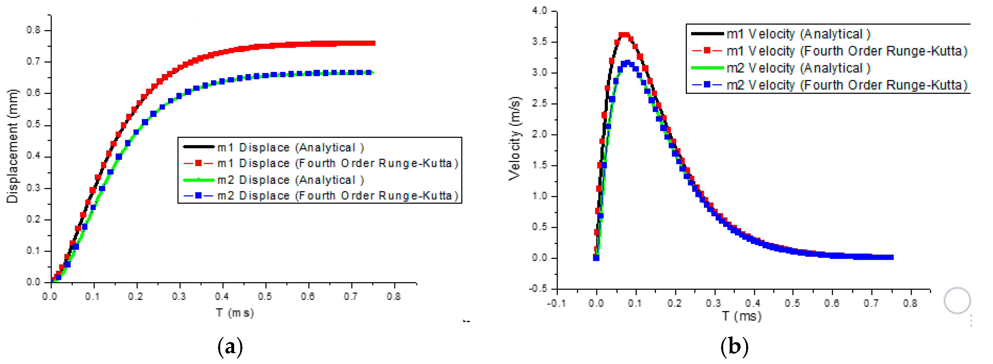
To ensure the accuracy of the inverse Laplace transform technique, we compared (Figure 4) the time histories of the x-displacement and the x-velocity of the left and the right plates, computed by the Laplace transform method with those values obtained from the Runge–Kutta method. It is evident that the two sets of results coincide with each other.
The water was assumed to separate from the plate when the pressure (or the normal traction) between the two decreases to zero, and the time of separation was defined as the cavitation time τc. The dependence of τc on the values of k and Cdamp is evidenced in Figure 5. For k and Cdamp equal to 105, τc decreased rather rapidly with an increase in the value of ϕ1, but for k and Cdamp equal to 107 or higher, τc seemed to approach a constant value of 0.21 ms for ϕ1 greater than 1.5.
The maximum impulse is given by , assuming that the system behaves as a rigid body. Equating impulse to the change in the linear momentum, we can find the ideal maximum velocity of the system if it were moving as a rigid body. For the present system, the maximum linear momentum can be found by computing the time history of (m1 + m2). The ratio of the maximum momentum achieved to the maximum impulse equals the momentum transmission coefficient ζ, which is a quantitative measure of the interaction between the fluid and the structure, and takes values between 0 and 1. When the net pressure PT(t) decreases to zero at time τP, the plate will reach its peak response with momentum IP, where the net pressure acting on the system is the difference between PL(t) and PR(t), and can be estimated by:
The dependence of the time for the peak pressure and the momentum transfer coefficient on the FSI parameter ϕ1 is shown in Figure 6a,b. The results reveal that the time of the peak pressure and values of the momentum transfer coefficient did not depend on the damping coefficient and the spring constant, since the peak pressure was from fluids from the wet surface of the vessel, and theoretically, in one dimension, dissipation was not a concern, so the energy was completely absorbed by the vessel no matter the stiffness value and viscosity value of the vessel. For all values of k and Cdamp considered here, the momentum transfer coefficient and time of the peak pressure decreased rather rapidly with an increase in the value of ϕ1.
4. Parameter Prediction by BPNN
The back-propagation neural network (BPNN) was first introduced by Rumelhart and Hintonis [17], and then used for image recognition [18,19,20], parameter prediction [21] and optimising data fusion, [22,23]. The feed-forward back-propagation neural network was designed to train the matrix of input data of this problem, such as the stiffness, fluid–structure factor, and damping coefficients. To improve networks’ adaptation and generalisation ability, the architecture of the network model is constructed in the Matlab neural network training tool (nntraintool), as shown in Figure 7.
A three-layer feed-forward network with scaled conjugate gradient back propagation can classify vectors arbitrarily well, given enough neurons in its two hidden layers with a maximum epoch of 1000. The result was that the subjective choice of structural parameters was significantly reduced. Table 1 shows the parameters of BPNN predictions.
For the cavitation inception time τc, the matrix of the viscous coefficient of the dashpot, stiffness, and the FSI parameter ϕ1= 2ρcθ/m1 were counted as input layer parameters. It took 500 iterations for the results, achieving training loss no more than 0.0104%, which is acceptable accuracy. Figure 8a shows that the training results coincided with the validation results. Furthermore, Figure 8b shows that the BPNN prediction results agreed with the analytical solution.
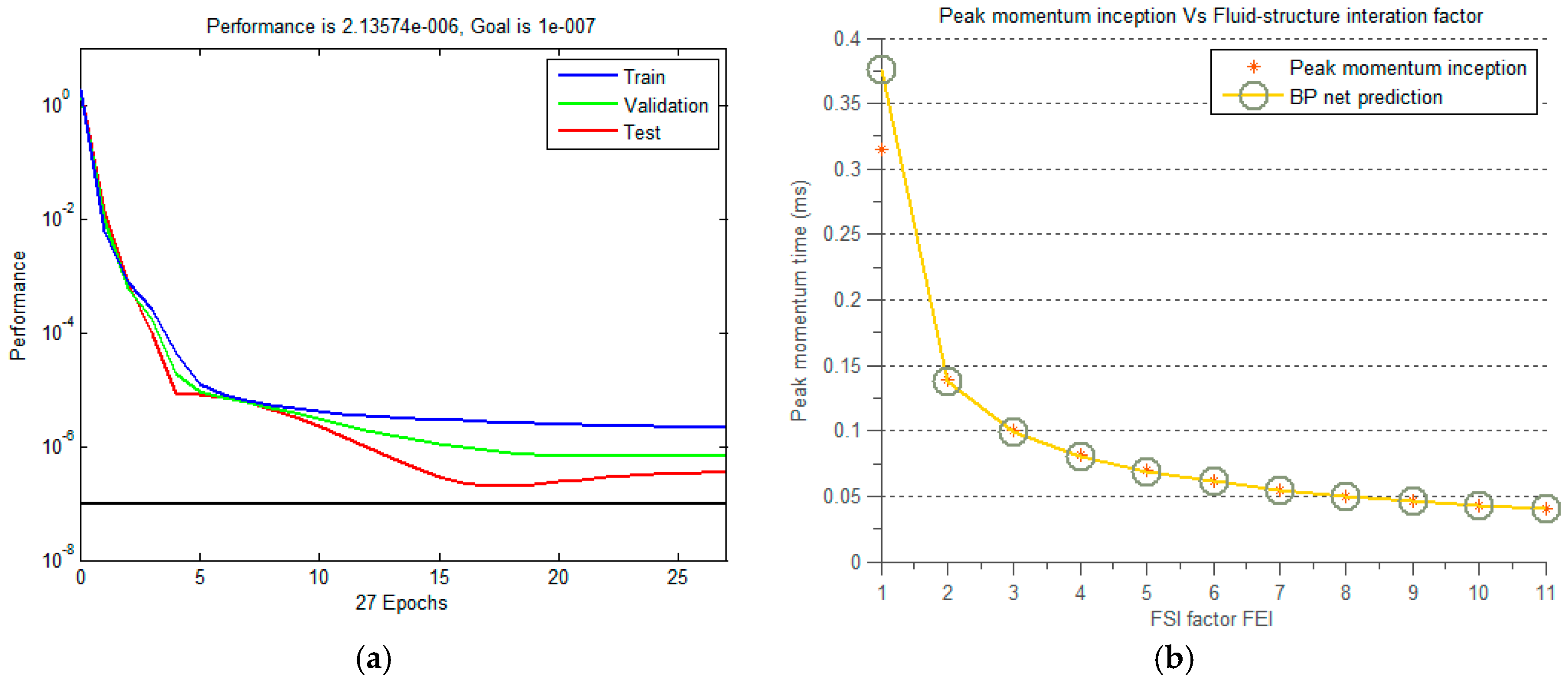
The training results of peak momentum time τP are shown in Figure 9. The deviation happens on the initial value of the FSI parameter ϕ, which shows that a small mass has more training loss.
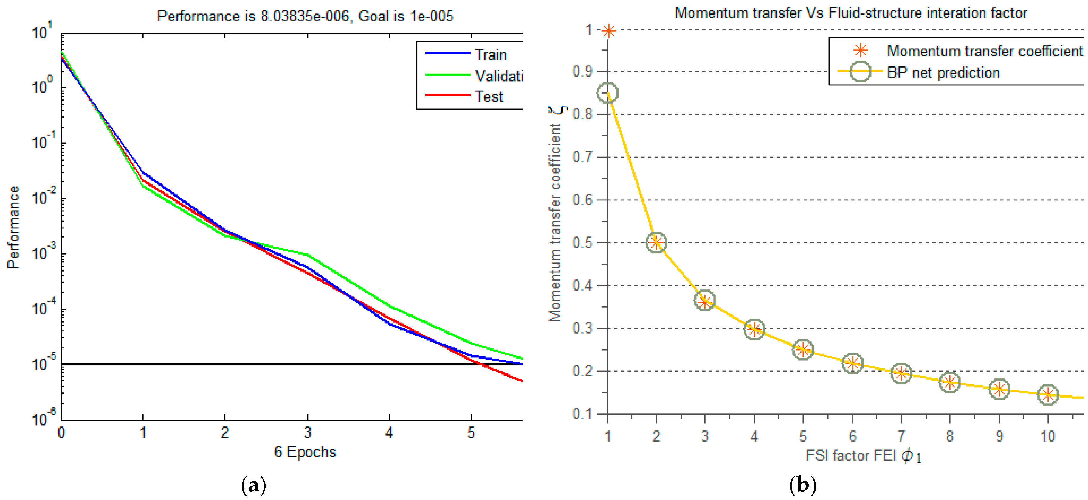
The training results of the momentum transfer coefficient vs. the FSI parameter ϕ1 = 2ρcθ/m1 are shown in Figure 10. The training curve shows excellent agreement with the validation and test sample results. The momentum transfer coefficient exhibits more deviation when training with small mass parameters.
5. Finite Element Analysis
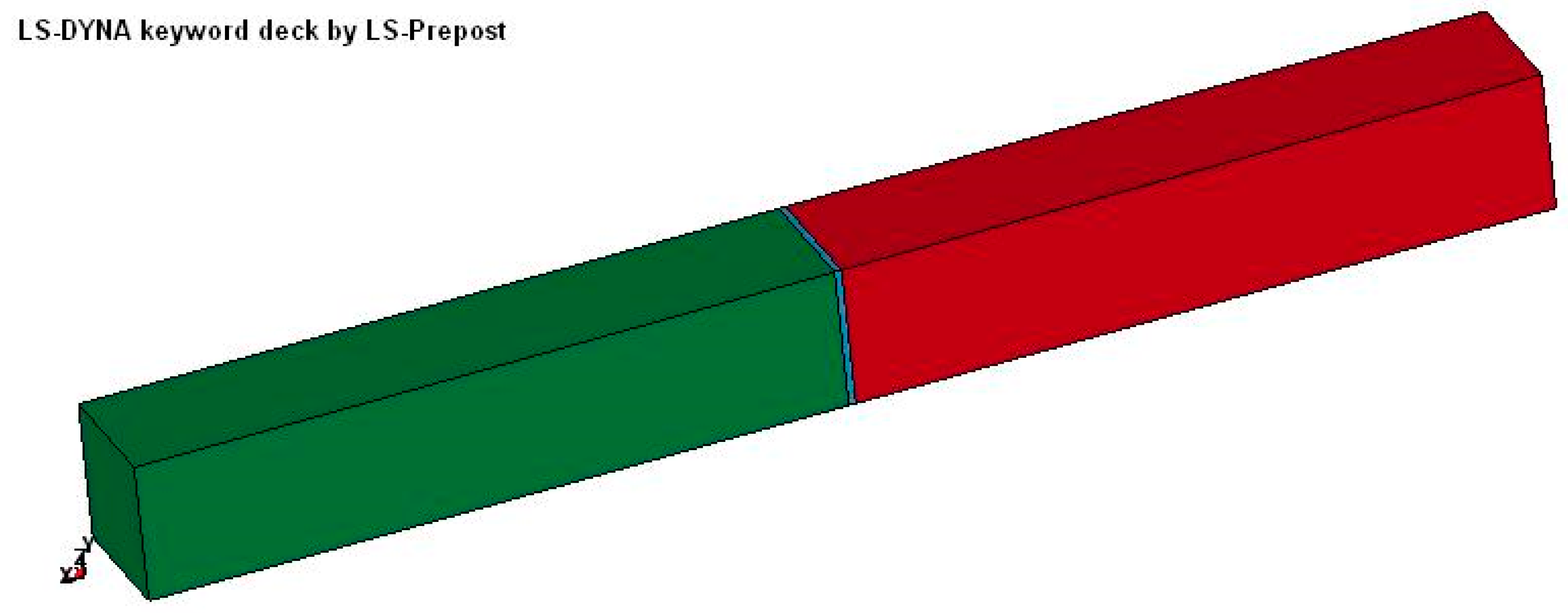
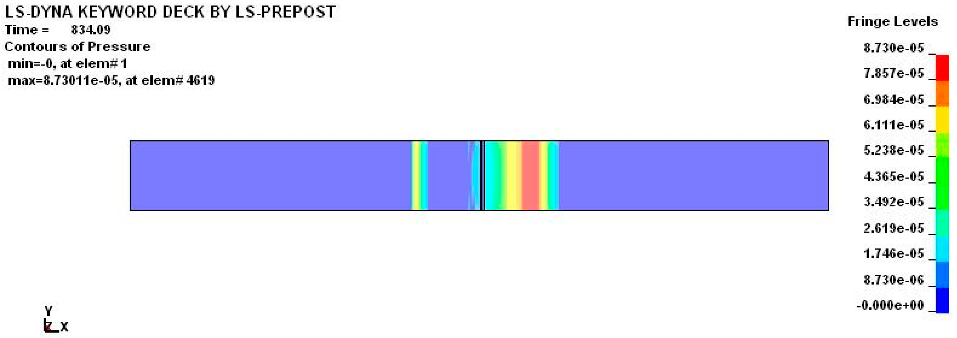
The commercial code LSDYNA was used to calculate the problems of Taylor’s model, as well as the generalized model. In LSDYNA, solid elements were used to model the bar in the configuration shown in Figure 11. On the cross section of the fluid bar, the solid elements were 0.2 m × 0.2 m squares, and the x-direction length of the elements was within 1 m of each side of the rigid plate. To model the problem as one dimensional, the nodes on the fluid bar were constrained so that only the motion in the x-direction was allowed. The calculation of the one-dimensional shock-wave is shown in Figure 12 and the wet surface pressure of different plate masses subjected to the underwater shockwave is shown in Figure 13.
The analytical solution (Taylor, 1949) to a rigid plate floating at water level subjected to the underwater shock waves was compared with a numerical solution by the LSDYNA code. The problem was modelled as two columns of fluid connected to the two faces of one rigid plate. Each column had a length of one meter, and the materials in the model were water on the left and air on the right. Planar shock wave loads were assigned to the left end of the column, with all nodes moving in one direction along the x-axis. The results of the rigid plate’s motion are shown in Figure 14.
6. Conclusions
The architecture of the BPNN for parametric predictions of underwater explosion problems based on analytical and numerical results was proposed and validated in this study. Taylor’s analysis of the motion of a rigid plate has been extended, with one side exposed to water and the other to air, to the case of two rigid parallel plates interconnected by a spring and a dashpot. The system was immersed in water with an exponentially decaying plane wave striking the left plate at normal incidence. The motions of the two plates as a function of their masses, spring stiffnesses, and their damping coefficients, were computed. Assuming that the fluid cannot support any tensile pressure, the cavitation time, the dependence of the momentum transfer coefficient, and the cavitation time upon the fluid–structure parameter were quantified. For more complicated problems, we can further advance the machine-learning model using finite element method for training purposes. The machine-learning model can significantly reduce the computational resources required for three dimensional simulations of underwater explosions.
Author Contributions
Conceptualization, D.D.; Data curation, M.Z.; Formal analysis, L.L.; Methodology, D.D. and X.Y.; Supervision, D.D. and X.Y.; Writing—original draft, M.Z.; Writing—review & editing, D.D. and X.Y.
Conflicts of Interest
There is no conflict of interest.
References
- Taylor, G.I. The Pressure and Impulse of Submarine Explosion Waves on Plates; The National Archives: Richmond, UK, 1941; pp. 287–303.
- Liu, Z.; Young, Y.L. Transient Response of a Submerged Plate Subject to Underwater Shock Loading: An Analytical Perspective. J. Appl. Mech. 2008, 75, 1–5. [Google Scholar] [CrossRef]
- Kambouchev, N.; Noels, L.; Radovitzky, R. Nonlinear Compressibility Effects in Fluid-Structure Interaction and Their Implications on the Air-Blast Loading of Structures. J. Appl. Phys. 2006, 100, 063519. [Google Scholar] [CrossRef]
- Kambouchev, N.; Radovitzky, R. Fluid-Structure Interaction Effects in the Dynamic Response of Free-Standing Plates to Uniform Shock Loading. ASME J. Appl. Mech. 2007, 74, 1042–1046. [Google Scholar] [CrossRef]
- Kambouchev, N.; Noels, L.; Radovitzky, R. Numerical Simulation of the Fluid-Structure Interaction Between Air Blast Waves and Free-Standing Plates. Comput. Struct. 2007, 85, 923–931. [Google Scholar] [CrossRef]
- Tan, P.J.; Reid, S.R.; Harrigan, J.J. Discussion: The Resistance of Clamped Sandwich Beams to Shock Loading. ASME J. Appl. Mech. 2005, 72, 978–979. [Google Scholar] [CrossRef]
- Hutchinson, J.W.; Xue, Z. Metal Sandwich Plates Optimized for Pressure Impulses. Int. J. Mech. Sci. 2005, 47, 545–569. [Google Scholar] [CrossRef]
- Schechter, R.S.; Bort, R.L. The Response of Two Fluid-Coupled Plates to an Incident Pressure Pulse; Technical Report No. 4647; Naval Research Laboratory: Washington, DC, USA, 1981. [Google Scholar]
- Hallquist, J.O. LS-DYNA THEORETICAL MANUAL; California, Livermore Software Technology Corporation: Livermore, CA, USA, 1998. [Google Scholar]
- Mindlin, R.D.; Bleich, H.H. Response of an Elastic Cylindrical Shell to a Transverse Step Shock Wave. ASME J. Appl. Mech. 1953, 26, 189–195. [Google Scholar]
- Haywood, J.H. Response of an Elastic Cylindrical Shell to a Pressure Pulse. Q. J. Mech. Appl. Math. 1958, 11, 129–141. [Google Scholar] [CrossRef]
- Huang, H. Transient Interaction of Plane Acoustic Waves with a Spherical Elastic Shell. J. Acoust. Soc. Am. 1969, 45, 661–670. [Google Scholar] [CrossRef]
- Huang, H. An Exact Analysis of the Transient Interaction of Acoustic Plane Waves with a Cylindrical Elastic Shell. ASME J. Appl. Mech. 1970, 37, 1091–1099. [Google Scholar] [CrossRef]
- Huang, H. Transient Response of Two Fluid-Coupled Spherical Elastic Shells to an Incident Pressure Pulse. J. Acoust. Soc. Am. 1979, 65, 881–887. [Google Scholar] [CrossRef]
- Zhang, P.; Geers, T. Excitation of a Fluid-Filled, Submerged Spherical Shell by a Transient Acoustic Wave. J. Acoust. Soc. Am. 1993, 93, 696–705. [Google Scholar] [CrossRef]
- Jones-Oliveira, J. Transient Analytic and Numerical Results for the Fluid-Solid Interaction of Prolate Spheroidal Shells. J. Acoust. Soc. Am. 1996, 99, 392–407. [Google Scholar] [CrossRef]
- Rumelhart, D.E.; Hinton, G.E.; Williams, R.J. Learning representations by back-propagating errors. Nature 1986, 323, 533–536. [Google Scholar] [CrossRef]
- Szegedy, C.; Liu, W.; Jia, Y.; Sermanet, P.; Reed, S.; Anguelov, D.; Erhan, D.; Vanhoucke, V.; Rabinovich, A. Going deeper with convolutions. arXiv 2014, arXiv:1409.4842. [Google Scholar]
- Simonyan, K.; Zisserman, A. Very deep convolutional networks for large-scale image recognition. In Proceedings of the International Conference on Learning Representations, ICLR 2015, San Diego, CA, USA, 7–9 May 2015. [Google Scholar]
- Veit, A.; Wilber, M.J.; Belongie, S. Residual networks behave like ensembles of relatively shallow networks. In Proceedings of the 30th International Conference on Neural Information Processing Systems, Barcelona, Spain, 5–10 December 2016; pp. 550–558. [Google Scholar]
- Dai, Y.C.; Huang, D.K.; Xu, J.W. Optimization of Characteristic Parameters of Pipeline Crack Identification Based on BP Neural Network. Adv. Mater. Res. 2014, 926–930, 3442–3446. [Google Scholar] [CrossRef]
- Mao, Z.; Zhang, Z.R.; Lu, Y.L. The Data Fusion in Multi-Sensors Grain Information Monitoring System Based on Improved BP Neural Networks. Appl. Mech. Mater. 2013, 263–266, 269–276. [Google Scholar] [CrossRef]
- Lu, Y.Y. Performance Study of BP Neural Network Based on PK Algorithm. Comput. Syst. Appl. 2019, 28, 173–177. [Google Scholar]
Figure 1.
(a) Schematic and (b) simple model of the problem studied. P(L), left plate; P(R), right plate.
Figure 1.
(a) Schematic and (b) simple model of the problem studied. P(L), left plate; P(R), right plate.

Figure 2.
Time histories of (a) the displacement of the left plate for different values of Cdamp and k, and (b) the pressure PLw on the left plate, PRw on the right plate, and the internal force/area, FCK.
Figure 2.
Time histories of (a) the displacement of the left plate for different values of Cdamp and k, and (b) the pressure PLw on the left plate, PRw on the right plate, and the internal force/area, FCK.

Figure 3.
For different values of Cdamp and k, time histories of (a) the speed, and (b) the acceleration of the left plate.
Figure 3.
For different values of Cdamp and k, time histories of (a) the speed, and (b) the acceleration of the left plate.

Figure 4.
Comparison of analytical and numerical solutions for time histories of (a) the displacement and (b) the velocity of the two plates.
Figure 4.
Comparison of analytical and numerical solutions for time histories of (a) the displacement and (b) the velocity of the two plates.

Figure 5.
For different values of Cdamp and k, the dependence of the cavitation time on the non-dimensional parameter ϕ1.
Figure 5.
For different values of Cdamp and k, the dependence of the cavitation time on the non-dimensional parameter ϕ1.

Figure 6.
(a) Dependence of the peak momentum time and (b) the momentum transfer coefficient upon the fluid–structure interaction (FSI) parameter ϕ1=2ρcθ/m1.
Figure 6.
(a) Dependence of the peak momentum time and (b) the momentum transfer coefficient upon the fluid–structure interaction (FSI) parameter ϕ1=2ρcθ/m1.

Figure 7.
The architecture of the network model in the Matlab neural network training tool.

Figure 8.
Training process performance curve (a) and comparison of the BP neural network prediction with the analytical results (b).
Figure 8.
Training process performance curve (a) and comparison of the BP neural network prediction with the analytical results (b).

Figure 9.
Training process performance curve (a) and comparison of the peak momentum time τP with the prediction results (b).
Figure 9.
Training process performance curve (a) and comparison of the peak momentum time τP with the prediction results (b).

Figure 10.
Training process performance curve (a) and the BP neural network prediction of momentum transfer (b).
Figure 10.
Training process performance curve (a) and the BP neural network prediction of momentum transfer (b).

Figure 11.
The model in LSDYNA for Taylor’s problem. The rigid plate with water on one side and with air on the other side.
Figure 11.
The model in LSDYNA for Taylor’s problem. The rigid plate with water on one side and with air on the other side.

Figure 12.
The one-dimensional shock wave calculation (pressure contours) of Taylor’s Problem using LSDYNA.
Figure 12.
The one-dimensional shock wave calculation (pressure contours) of Taylor’s Problem using LSDYNA.

Figure 13.
The wet surface pressure of different plate masses subjected to the underwater shockwave (Taylor’s model).
Figure 13.
The wet surface pressure of different plate masses subjected to the underwater shockwave (Taylor’s model).

Figure 14.
Comparison between the results of Taylor’s analytical solution and that of LSDYNA.


Table 1.
BPNN and structure parameters for calculation.
| Algorithm | Layers | Epoch | Stiffness k | Damping C | FSI Parameter ϕ |
|---|---|---|---|---|---|
| Gradient Descent with Momentum | Input | 500 | 103 | 103 | 0.2 to 20 |
| Hidden layer 1 | 105 | 105 | |||
| Hidden layer 1 | 106 | 106 | |||
| Output layer | 107 | 107 |
© 2019 by the authors. Licensee MDPI, Basel, Switzerland. This article is an open access article distributed under the terms and conditions of the Creative Commons Attribution (CC BY) license (http://creativecommons.org/licenses/by/4.0/).
Share and Cite
MDPI and ACS Style
Zhang, M.; Drikakis, D.; Li, L.; Yan, X. Machine-Learning Prediction of Underwater Shock Loading on Structures. Computation 2019, 7, 58. https://0-doi-org.brum.beds.ac.uk/10.3390/computation7040058
AMA Style
Zhang M, Drikakis D, Li L, Yan X. Machine-Learning Prediction of Underwater Shock Loading on Structures. Computation. 2019; 7(4):58. https://0-doi-org.brum.beds.ac.uk/10.3390/computation7040058
Chicago/Turabian StyleZhang, Mou, Dimitris Drikakis, Lei Li, and Xiu Yan. 2019. "Machine-Learning Prediction of Underwater Shock Loading on Structures" Computation 7, no. 4: 58. https://0-doi-org.brum.beds.ac.uk/10.3390/computation7040058
Note that from the first issue of 2016, this journal uses article numbers instead of page numbers. See further details here.